Abstract
The time-triggered communication paradigm is a cost-efficient way to meet the real-time requirements of cyber-physical systems. It is a non-deterministic polynomial NP-complete problem for multi-hop networks and non-strictly periodic traffic. A two-level scheduling approach is proposed to simplify the complexity during optimization. In the first level, a fuzzy-controlled quantum-behaved particle swarm optimization (FQPSO) algorithm is proposed to optimize the scheduling performance by assigning time-triggered frame instances to the basic periods of each link. In order to prevent population from high aggregation, a random mutation mechanism is used to disturb particles at the aggregation point and enhance the diversity at later stages. Fuzzy logic is introduced and well designed to realize a dynamic adaptive adjustment of the contraction–expansion coefficient and mutation rate in FQPSO. In the second level, we use an improved Satisfiability Modulo Theories (SMT) scheduling algorithm to solve the collision-free and temporal constraints. A schedulability ranking method is proposed to accelerate the computation of the SMT-based incremental scheduler. Our approach can co-optimize the jitter and load balance of communication for an off-line schedule. The experiments show that the proposed approach can improve the performance of the scheduling table, reduce the optimization time, and reserve space for incremental messages.
1. Introduction
The cyber-physical system (CPS) is the next-generation engineering system to realize a deep integration of computing, communication, and control technology. Its core technology is the close integration of information systems and physical units, which are considered prospects of a networked control system [1]. Physical units act on the control process of automation in the cores of embedded devices, while information systems make full use of communication facilities and resources to acquire, transfer, and apply CPS instructions and information.
The main difficulty of CPS control lies in the co-scheduling of the physical unit and the information system [2,3]. The sampling and control processes of physical units are run on spatially distributed entities, including controllers, actuators, and sensors, and these are generally divided into periodic embedded task sets which have precedence constraints, different rate intervals, strict deadlines, and jitter requirements. Under non-preemptive communication protocol, it is necessary to efficiently co-schedule tasks of physical and information systems to maximize the utilization of network facilities and resources. Instead of a low speed and low bandwidth fieldbus, the communication process of an information system can be undertaken by switched real-time Ethernet (RTE) protocols governed by IEC 61850 [4] and IEC 61158 [5], which make co-scheduling problems more complicated.
Scheduling problems are generally considered as restricted resource allocation problems with specific dependencies and constraints, which can be addressed using a constraint programming approach. Two types of approaches are formally defined: constraint satisfaction problems (CSPs) and constraint optimization problems (COPs) [6]. The purpose of CSPs is to achieve the satisfiability of a set of constraints, while COPs aim at optimizing an objective function on the basis of constraints satisfaction. In time-triggered CPS scheduling, the hard real-time constraints include the period, deadline, precedence, etc., which must be satisfied while some quality of service (QoS) parameters, such as the jitter, latency and load balance of the scheduling table, can be optimized by COP to improve the communication performance.
A multitude of optimal and heuristic techniques have been developed to solve COPs in time-triggered scheduling. The main problem is the complexity of non-deterministic polynomial (NP) complete, which limits the scale of networks and communication tasks. Although advanced methods and algorithms are proposed in past and recent references, it is still a hot topic in the field of optimization theory.
The scheduling optimization of non-strictly periodic traffic further aggravates the NP-complete problem. In recent research and articles, most of the studies are focused on strictly periodic scheduling, which only needs to schedule the first periodic frame instance of traffic flow. However, allowing non-strictly periodic frames can refine the granularity of the schedule table from flow level to frame level and thus heavily improve the solution space and flexibility.
2. Related Works
The survey article [7] proposes a mathematical modeling framework that sets forward fundamental challenges in sensing, decentralized computation, robustness, energy efficiency, and hardware security in CPS. Many references have explained in detail how the design and scheduling of information systems affect the control process and stability of CPS. Derler [8] and Poovendran [9] analyze the real-time and synchronization characteristics of CPSs, which must be guaranteed. Karsai [10] introduces a joint modeling method of an embedded system based on the dynamic integration of software and physics. Xiaofeng Yu [2] focuses on the information transmission path on physical systems and finds an optimal path to meet the requirement of physical system stability. The influence of information system delay on physical process is studied. Bradley [3] establishes control models for an information system and physical system, respectively. Taking the sampling time as the research object, an optimal control of computational–physical state co-regulation is studied in CPS. The results show that CPS needs industrial communication protocol and a real-time scheduling scheme to integrate information and physical systems.
According to the characteristics and services of a control system, the scheduling methods of tasks among multicores or multi-agents in CPSs are also very different. For physical processes that have high variability, non-Gaussianity, and higher order spatiotemporal correlations in personalized medicine, Bogdan defines a cyber-physical task graph as a time-dependent representation and proposes a goal-oriented self-optimization inspired solution for resource allocation on Network-on-Chip-based multicore platforms [11]. In industrial applications, such as aircraft, high-speed trains, power grids, etc., real-time scheduling methods of fieldbus and distributed communication systems (Lonworks [12], WorldFIP [13], CAN [14], FlexRay [15], etc.) have been widely studied in industrial control applications. Moreover, using Ethernet and transmission control protocol/Internet protocol (TCP/IP) technologies to integrate a local area network (LAN) in CPSs allows utilities to be interconnected with automation networks, which has features such as high bandwidth, openness, wide availability, and low cost [16,17]. Although this work focuses on fully switched real-time Ethernet, it can also be used in fieldbus protocol or another switched real-time industrial network by extension. The inherently non-deterministic carrier-sense with collision detection (CSMA/CD) mechanism conditioned the adoption of Ethernet in time-critical applications [18]. To overcome those shortcomings, several real-time protocols have been introduced to enforce time-critical communication over Ethernet [19]. One cost-efficient way is the time-triggered scheduling, which plans transmission points of frames off-line.
Some articles, such as [20,21,22] propose QoS-based design methods for fieldbus networks with the bandwidth allocation described as multi-objective optimization problems. Natale [23] solves the problem with an objective to minimize the jitter of activities using simulated annealing. However, the time complexity of NP-complete will become more prominent with the increase of network and traffic scale. The algorithms in these references are only applicable to fieldbus scenarios and are difficult to work at full capacity in a multi-hop switched Ethernet.
Many related studies have done a lot of work to realize real-time Ethernet scheduling. A rate-monotonic algorithm has been used to accelerate scheduling time in [24,25]. The tabu search algorithm has been used to design the scheduling table off-line and improve the overall real-time performance by reducing the packet delay of rate-constrained frames in [26,27]. The pinwheel scheduling solution [28] is regarded as a relaxation of the jittered-bounded scheduling concept, where each activity is required to be scheduled at least once during each predefined number of consecutive time units. Hanzalek in [29] introduces a resource-constrained project scheduling with temporal constraints to minimize the Profinet IO IRT scheduling makespan. However, the jobs are aperiodic and executed only once in a macro period. A formal specification of scheduling constraints for time-triggered multi-hop networks and strictly periodic traffic while solving with the Satisfiability Modulo Theories (SMT) solver is introduced in [30,31,32,33]. The strictly periodic model leads to a relatively lower resource utilization and flexibility. Besides, frame constraints are added into the solver without considering the urgency and schedulability of frames. Therefore, the computation time of the schedule table increases rapidly with the number of constraints. In large-scale or non-periodic scheduling, it is hard to get a feasible solution within a time limit. A jitter satisfaction problem is solved by a three-level greedy algorithm in [34]. A strictly periodic multi-cluster scheduling approach is proposed in [35] by dividing flows into intra-cluster and inter-cluster. The off-line and on-line algorithms are presented to fast react to cluster-level changes in networks. A novel search-space pruning technique based on the response times is proposed in [36] to generate a schedule for large distributed time-triggered systems within a reasonable amount of time. Due to the NP-complete of multi-hop scheduling, most of the researches are aimed at increasing the scheduling scale and reducing the scheduling time in strictly periodic scheduling while satisfying the constraints. The optimization of scheduling performance with non-strictly periodic traffic has not been fully studied.
The classic particle swarm optimization (PSO) is not a global optimization algorithm. Sun et al. [37] introduces quantum theory into a PSO algorithm and proposes a quantum-behaved particle swarm optimization (QPSO). The contraction–expansion coefficient is the only parameter in QPSO that needs to be set manually besides the population size, particle dimension, and maximum iteration times. Its control strategy has a great influence on the performance of the algorithm. Sun proves that the contraction–expansion (CE) coefficient must be less than 1.781 in order to make the particles converge reliably. The dynamic non-linear decreasing control strategy of the CE coefficient is proposed in [38]. According to the characteristics of different optimization problems, different control curves with concavity and convexity are adopted. However, fixed, linear or non-linear decreasing are all non-feedback control strategies that are obtained by simulation experiments or empirical formulas. This kind of coefficient control strategy has weak self-regulation ability. It cannot adjust the coefficient according to the change of search stage. Liu proposes a novel dynamic CE coefficient for QPSO involving two factors, namely, the evolution speed factor and aggregation degree factor in [39], which can be modified on-line. The fuzzy logic control is one of the most popular control techniques, and it is often used to adjust the parameters of control systems or other algorithms adaptively. The fuzzy logic control is applied in numerous mixes with other algorithms such as the fuzzy logic for inertia weight particle swarm optimization in [40], immune particle swarm optimization in [41], neural networks in [42], model-free adaptive control in [43], and virtual reference feedback tuning in [44]. At present, we have not seen the work of using fuzzy control logic to adaptively control the CE coefficient in QPSO.
This article starts with an introduction of the situation and difficulty of CPS periodic scheduling. Section 2 discusses the related works. A multi-objective optimization problem of non-strictly periodic scheduling in CPS based on time-triggered multi-hop network is proposed in Section 3 for first-level scheduling. A fuzzy-controlled quantum-behaved particle swarm optimization (FQPSO) algorithm for adaptive parameter selection is proposed in Section 4. Section 5 introduces an improved incremental scheduler based on the SMT solver and schedulability ranking of frames to accelerate computation. The experiments and performance discussion are presented in Section 6. This article finishes with conclusion.
This work is different in that it is the first to propose a two-level scheduling approach, which includes optimization and satisfiability parts, to simplify NP-complete complexity. It is also the first to define the load balance of message distribution in the macro cycle in order to improve an incremental schedule of periodic time-triggered messages. Fuzzy logic is firstly used to adaptively adjust CE coefficients in QPSO. An innovation of schedulability ranking in an incremental SMT solver is proposed to solve the problem of excessive callbacks in previous work.
3. Scheduling Optimization
3.1. System Model
This article improves an Ethernet train communication network (TCN) topology in IEC61375-3-4 [45] as an application platform. TCN is a typical real-time CPS, whose topology is hierarchical with one or more train backbone subnets and one or more Ethernet consist network (ECN) subnets. Train backbone nodes (TBN) and links along the train are used to connect active ECN subsets together, while the ECN interconnects end devices (ED) located in one consist and transmits data frames between EDs and between EDs and TBNs through consist network nodes (CNNs) and links. We assume links as full duplex connecting multiprocessor nodes to transmit messages between devices in both directions. Each ED contains a set of homogeneous cores on an electronic control unit (ECU) with output and input ports acting as communication end points that can send or receive only one single message at a time.
The work of this paper is based on time-triggered improved Ethernet and focus on non-strictly periodic process data in TCN. The communication management, routing protocol, communication layer model, and packet format of TCN in our work are regulated by IEC 61375-2-3 [46], which defines a state-of-the-art protocol based on switched Ethernet named train real-time data protocol (TRDP). Our work focuses on the optimization of a static scheduling table that is not confined to specific protocol and is easily extensible to other distributed control system communication networks such as bus, mesh, wireless communication, and so on. Similarly, on the premise of network clock synchronization and determined message routing, the structure of network topology, such as a ring, a tree, or a star, or redundant structures as parallel and ladder structures in IEC 61375-3-4, does not affect the optimization model, analysis, and conclusion of this paper.
The proposed communication topology in this article is shown in Figure 1. A ring topology is formed by three switches and five devices distributed in it. Formally, the physical topology of the information system in CPS can be depicted by a directed graph G (V, E), where V = ED ∪ CNN contains all the EDs and CNNs, and E is the set of physical links. One physical link consists of two dataflow links in opposite directions. A dataflow link lk ∈ L represents a directed communication link between two adjacent nodes, and L is the set of dataflow links in a network. A dataflow path dpi is formed by an ordered sequence of lk connecting one sender to one or several receivers. For example, the dataflow path dp1 is depicted by a dotted line from ED1 to ED5, which can be also denoted as the ordered lk sequence, i.e., l1→l5→l9 in Figure 1.
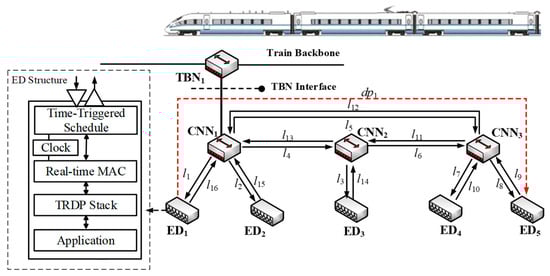
Figure 1.
Topology of the proposed information system in a cyber–physical system (CPS).
All the source and sink ports of EDs in the fieldbus network share the common collision domain so that only one port can occupy the physical link for message transmission. As switched Ethernet is isolated from ports of switches to their respective collision domains, the ports of all EDs can send or receive messages at the same time. When there is no overlap of dataflow paths, i.e., dp1 ∩ dp2 ∩…∩ dpn = ∅, messages can be scheduled as several independent fieldbuses at the same time in the network. Otherwise, dp1 ∩ dp2 ∩…∩ dpn ≠ ∅, and overlapped links should be co-scheduled through the store and forward mechanism of Ethernet switches, as long as the end-to-end delay can meet the deadline requirements of messages, which enhances the flexibility and utilization of the network.
In Figure 1, communication between source and sink EDs is distributed globally by dataflow paths and relayed through switches. Messages need to go through several dataflow links during the transmission process. Due to the collision domain isolation characteristics of switch ports, the transmission of messages can be divided into a series of frame instances.
The communication between CPS physical units is undertaken by messages. Assume that a periodic message is transmitted in the payload of a dedicated frame fi. We denote the set of all frames by F with fi ∈ F. For each frame, the prior attributes are given as shown in Equation (1):
where ri is the release time, which specifies the earliest time that a message can be sent from source ED. di is the message deadline, which represents the absolute time from 0 moments to the moment when a message is completely received by its destination. ei is the end-to-end deadline from the moment when a data frame is sent from source ED to the moment when it is completely received by its destination. pi is the amount of time that the frame of the message occupies the dataflow link, and Ti is the time period of the message. N is the number of frames.
Under synchronization, the global network communication time is divided into macro periodic units denoted by TMp, which is equal to the least common multiple (LCM) of all the message periods in the network. In addition, each link has its own basic period denoted by Tbp, which is equal to the greatest common divisor (GCD) of the message periods on this link. TMp is an integral multiple of Tbp.
3.2. Objective Function
In order to ensure the real-time performance of time-triggered periodic messages as well as keep more free time slots in the basic periods, the optimization target concentrates on the frame jitter, transmission delay, and load balance of the macro period in the k-th link. In a multi-hop non-strictly periodic scheduling problem, it is usually difficult to satisfy the collision-free constraints through optimization. In this section, we firstly assign frame instances to basic periods, regardless of their overlapping issues.
s(i, j, lk) and s(i, j + 1, lk) are the sending time of the j-th and (j + 1)-th instances of frame fi on dataflow link lk. M is the number of frames on lk. The sum of jitters on lk can be formulated as shown in Equation (2).
The periodic frames should be distributed uniformly so as to prevent data overflow and improve the load more balanced for incremental scheduling. The standard deviation of basic period utilization in a macro period can be used to define the load balance and is given by Equation (3):
where Nk is the number of basic periods in one macro period on lk and equals to TMp/Tbp,k, TMp is the macro period, and Tbp,k is the basic period for lk. , if any frame instance of fi is located in the r-th basic period, pi(r) equals the link occupancy time of fi. Otherwise, pi(r) = 0.
For every message flow, the sending time offset of frames should satisfy not only the constraints on the application level but also on the network level. The temporal constraints of the network are divided into eight types and analyzed in detail [28]. In this article, we use a directed graph to describe them formally. In order to facilitate description, five messages are assumed with their prior attributes defined in Equation (1) shown in Table 1, while the directed graph G is formed as shown in Figure 2.

Table 1.
Tasks and temporal constraints of periodic messages. ED: end device.
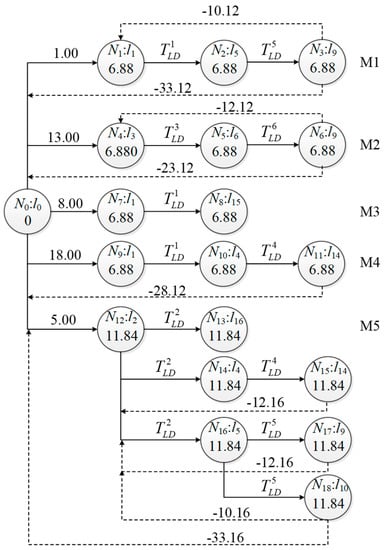
Figure 2.
Directed graph of task scheduling chart based on temporal constraints.
The link occupancy time pi = len × bTD + TGAP, where len is the frame length in bits. bTD is the single bit transmission time, which is approximately set as 0.01 μs, and TGAP is the inter-message protection interval with the value of 1.12 μs in this case. For example, if the unicast M1–M4 length is 72 bytes long and multicast M5 is 134 bytes long, we have p1-4 = 6.88 μs, p5 = 11.84 μs.
In Figure 2, there are 19 tasks in total marked by Nx with x from 0 to 18. N0 marks the start time of the system, and the link occupancy time is 0. The positive weight of the directed edges between the task nodes in Figure 2 is depicted as representing the link delay TLD on lk, which consists of two parts: physical links and connected switches. The positive weight between N0 and the first task node of message transmission represents the release time ri. The negative weight between the last task node and N0 is given by and indicates the absolute deadline of the frame from 0 moments. The negative weight between the last and first task node is given by and indicates the end-to-end deadline of each message.
The weight of the directed edges in Figure 2 forms a matrix W, which represents all the temporal constraints of frame instances during scheduling, as shown in Equation (5). Nx and Nx’ are tasks in Figure 2 with . The element ‘*’ in W indicates that the tasks of Nx and Nx’ have no constraint relations. The temporal constraints can be formalized as:
Therefore, ∀ lk ∈ L, the final objective function can be expressed as shown in Equation (6).
where F(lk) is the objective function of lk, J(lk) is the overall jitter value given by Equation (2), and J(lk)max and J(lk)min are the maximum and minimum value of J(lk), respectively. B(lk) is the standard deviation of basic period utilization in a macro period of lk given by Equation (3), and Bmax and Bmin are the maximum and minimum value of B(lk), respectively. a1 and a2 are the normalized weight coefficients. The first constraint means that the basic period Tbp,k should not overflow with frames. The second constraint is the temporal constraint given by Equation (4).
4. Fuzzy-Controlled Quantum-Behaved Particle Swarm Optimization
4.1. Quantum-Behaved Particle Swarm Optimization
QPSO assumes that the evolutionary system of a PSO algorithm is a quantum system. The aggregation can be described by bounded states existing in the center of particle motion, which is generated by the attraction potential well. Particles in quantum-bounded states can appear at any point in space with a certain probability density.
The exact values of positions and velocity cannot be determined simultaneously with quantum particles. In an N-dimensional search space, the QPSO algorithm consists of M particles representing potential solutions of the problem. At moment t, the relevant variables of the i-th particle are defined as follows with i takes an integer from 1 to M.
- Particles have no velocity vector;
- Position vector is ;
- Particle best position is ;
- Global best position is ;
- Attractor’s vector is ;
Sun et al. [35] present the basic theory and formula of QPSO. Considering that the particle’s position Xi,j(t), its local attractor pi,j(t), the characteristic length of potential well Li,j(t), and the random variable ui,j(t) develop with the iteration number n, the j-th component of the position of the i-th particle in the (t+1)-th iteration is given by Equation (7).
where , α(t) is the contraction–expansion (CE) coefficient to adjust the convergence rate of particles.
To ensure the convergence of QPSO, each particle must converge to its own local attractor pi,j(t) given by Equation (8), and must be satisfied.
where and are local and global learning factors,.
The control strategy of Li,j(t) is the key to affect the convergence and performance of QPSO. The typical Li,j(t) control method is to regulate the distance among particles and the mean best position C(t) is given by Equation (9).
The value of Li,j(t) can be given by Equation (10).
Therefore, the final evolution equation of QPSO is given by Equation (11).
4.2. Fuzzy-Controlled Adaptive CE Coefficient
The relationship between the CE coefficient α(t) and potential well length L(t) is discussed in [35]. The simulation results show that α(t) directly affects the length of L(t) and restricts the searching range of particles. When α(t) and L(t) are large, particle swarm has a strong global searching performance. Otherwise, the local searching performance is enhanced. The fixed, linear, or non-linear strategy of coefficients did not consider the relationship between α(t) and particle positions. In this article, a control strategy of CE coefficient based on fuzzy logic is proposed.
We define a population diversity factor β(t) to show the dispersion degree of particles and then to indicate the change of the searching range of particles, as shown in Equation (12).
where R is the longest radius of the searching space, Xi,j(t) is the j-th component of the i-th particle, is the average value of the j-th component for all the particles, M is the population size, and N is the dimensionality of the problem.
When the optimization begins, the length of potential well L(t) tends to decrease gradually with particles moving to the global optimal position. A larger β(t) means a lower aggregation degree and thus leads to a faster moving speed of particles, larger α(t), and L(t). Otherwise, α(t) and L(t) will be smaller.
The fitness increment of Equation (6) is dF(t) and represents the change of fitness value for two successive generations, given by Equation (13):
where Fmax and Fmin are the maximum and minimum fitness values during iterations, respectively.
Different stages of population evolution are represented as TFQPSO, given by Equation (14):
where t and tmax are the current iteration number and maximum iteration number, respectively.
With iterations moving on, the diversity of the population inevitably degenerates in later stages of evolution, which makes particle swarm converge prematurely. In order to solve this problem, we propose a stochastic mutation strategy for particle swarm. This algorithm makes particles have the ability to deviate from original position and find a better solution in high-dimensional space.
In a searching space with a dimension of N, the mutation threshold of the algorithm is , while the mutation rate on the components of particle positions is , m = 1, 2, …, N. When mutation is executed, the new position of the j-th component in the i-th particle is given by Equation (15).
The fuzzy logic controller is designed as follows. The inputs of the controller include the population diversity β(t), fitness increment dF(t), and evolution state TFQPSO. The outputs of the controller are the incremental value of the mutation factor dρ and CE co-efficient dα.
According to the range of fuzzy variables and corresponding linguistic variables sets in Table 2 and Table 3, the membership function of each variable is shown in Figure 3. In a current iteration, the input of fuzzy logic controller β(t), TFQPSO, dF(t) are calculated according to Equations (12)–(14). The outputs dρ and dα are obtained by Figure 3 and updated by Equation (16). They are used to update the particle positions in Equation (11) for the next iteration in FQPSO.
Table 3.
Fuzzy linguistic variables set.
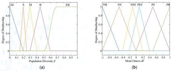
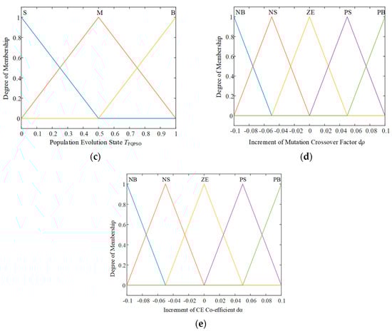
Figure 3.
The membership function for the (a) population diversity, (b) mean fitness, (c) population evolution state, (d) increment of mutation crossover factor, (e) increment of CE co-efficient.
5. Incremental Scheduler Based on SMT Solver
After FQPSO, frame instances are assigned to basic periods and meet the requirement of the objective function and constraints. However, since the collision-free constraints are not considered in the above process, frame instances will overlap each other in the table. The purpose of this section is to adjust the offset of frames to satisfy collision-free and temporal constraints in every basic period based on an improved SMT solver.
The FQPSO part greatly reduces the scale of collision-free constraints, which account for the majority of total constraints for the SMT solver. Delay and precedence can be constrained by Equations (4) and (5). The collision-free constraint is formally defined as shown in Equation (17):
where L is the set of dataflow links, the j-th basic period on dataflow link lk is denoted by , fv and fu are frame instances in , and are their sending offset, and pv and pu are their link occupancy times.
We propose an improved SMT solver to solve constraints (4), (5) and (17). This article defines the priority to decide the sequence of incremental frames scheduling. Not only the temporal urgency of frames, i.e., the end-to-end deadline in Figure 2, but also the interference of scheduled messages with unscheduled ones needs to be considered. The period utilization (PU) is defined as the bandwidth needed to transmit a frame fu on the premise that FQPSO has already allocated more urgent frame instances to basic periods, as given by Equation (18).
- means the bandwidth occupied by other frames except fu in the j-th basic period of dataflow link lk.
- means the fu transmission requires a fraction of time equal to pu every Tu time units.
Thus, the priority of each frame fu is set as a vector of two components priority = rank(min(eu), max(PUu)), where eu is the end-to-end deadline of fu and is compared firstly by the most critical parameter. PUu is compared secondly for frames that have the same end-to-end deadline. This priority value defines the difficulty of frame instance scheduling. The frame instance with less free scheduling space should be scheduled earlier. Figure 4 shows the incremental SMT scheduler based on the schedulability ranking in our approach.
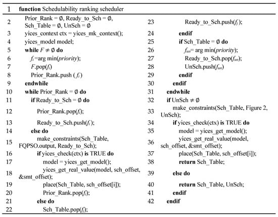
Figure 4.
The algorithm of an incremental Satisfiability Modulo Theories (SMT) scheduler.
Prior_Rank is the set of priority queues. Ready_to_Sch is the set of frames that are ready to schedule. Sch_table is the completed schedule table. UnSch is the set of unscheduling frames. Lines 5–9 are schedulability ranking approach, and these are used to compute the priority of frames and sort them to form the Prior_Rank queue. The lower priority is at the tail and the higher is at the head. In each iteration, the frame instance with the highest priority in the queue is added to Ready_to_Sch and scheduled by the SMT solver first.
Line 15 uses the frames in Ready_to_Sch, basic periods scheduling results from FQPSO, and offset of scheduled frames in Sch_table to generate SMT constraints and check whether the logic context is satisfiable (line 16). If so, the SMT solver gives a yices_model that satisfies the logic context (line 17) and returns the feasible solution into local array sch_offset from SMT pointer & smt_offset (line 18). The function place() in line 19 is used to explicitly add these time offset of frame instances to Sch_table. Then, the Prior_Rank is updated by deleting the successfully scheduled frame fi from the head of the queue.
If the current frame fi is not schedulable, the last successfully scheduled frame fj and its offsets are taken out of Sch_table and pushed back to Ready_to_Sch (lines 22–23). In the next iteration, fi and fj are scheduled together by lines 15–20 to find a feasible solution. If there is still no feasible solution when all the scheduled frames are popped out from Sch_table for backtracking, the frame with minimum priority fun is identified as a problematic frame and put into UnSch to prevent a scheduling crash (lines 25–31).
After all the frames in Prior_Rank are scheduled, the frames in UnSch are added to the SMT solver together and they check whether there is a feasible solution for them without considering the basic period limits from FQPSO. If so, the final schedule table Sch_table is returned. Otherwise, the Sch_table with currently scheduled frames and UnSch with unscheduled ones are returned.
After the two-level schedule is calculated, if there are a few messages newly adding into the system, the incremental SMT scheduler will be called to determine whether the idle time of the schedule table can meet the constraints of frames. When there is enough appropriate idle time, the scheduler will be updated with new frames online in several to hundreds of milliseconds. Otherwise, the schedule table needs to be recalculated off-line.
6. Experiment
6.1. Experiment Testbench
The experiment testbench is on a local machine with 8 GB memory and Ubuntu 16.10 operating system. We use an Intel(R) core (TM) i5-4590 3.3 GHz processor of Intel Corporation, America. The FQPSO algorithm is implemented by C++ language and the SMT solver is YICES 2.0.
The experimental process on the platform is shown in Figure 5.
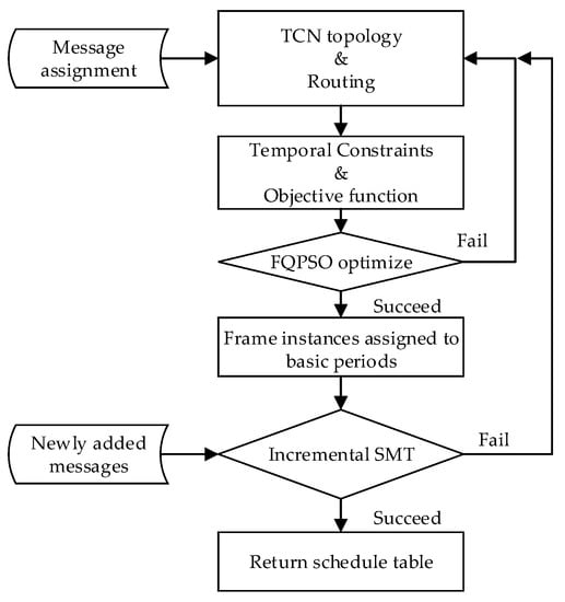
Figure 5.
Ethernet train communication network topology.
- Define message tasks and their attributes in TCN. In a realistic Ethernet TCN, the load is usually less than 50% of the total bandwidth. Under this, it is difficult to evaluate the performance of our approach. So, we use random traffic to simulate the network load.
- According to TCN topology, determine the route and dataflow path of messages.
- According to message attributes, delay parameters, and temporal constraints, complete the directed graph as Figure 2 and objective function.
- Use FQPSO to optimize the fitness of the objective function and assign frame instances to basic periods. If successful, continue scheduling. Otherwise, return to Step (2) to adjust the route and dataflow path.
- Call the incremental SMT scheduler to adjust the offset of frame instances in basic periods. If successful, output the time-triggered schedule table. Otherwise, return to Step (2) to adjust the route and dataflow path.
- When newly added messages are added to TCN, the incremental SMT is called for online scheduling. If successful, the schedule table is updated. Otherwise, return to Step (2) to recalculate the schedule table offline.
6.1.1. Topology
In the experimental section, we use an improved TRDP-based TCN system in a CR400 high-speed train of China as the realistic scheduling test platform, as shown in Figure 6. Each carriage is equipped with a consist network node (CNN), which adopts an industrial Ethernet switch and loads a time-triggered schedule table in it. Each CNN connects eight EDs and uses a ring topology to provide redundancy within the network. The train backbone node (TBN) uses a linear structure to connect two subnets. The topology contains 10 switches, 64 end devices, 75 physical links, and 150 directed dataflow links. The solid lines represent the Ethernet physical links, and the dotted lines represent the separation between two cars.

Figure 6.
Ethernet train communication network topology.
6.1.2. Message Assignments
Message assignment is done by generating dataflow paths each consisting of one sender and one or a set of receivers. In our testbench, a sender is randomly selected from all the EDs, and every message of the sender belongs either to a multicast group or a unicast group. A sender of multicast is allowed to transmit frames to a subset of a configurable group size of receivers. The unicast group is allowed only one receiver binding to a sender for the message. In this article, four types of time-triggered traffic are defined: (1) unicast within subnet: the source unicasts messages to one sink belong to the same TBN; (2) multicast within subnet: the source multicasts messages to 8–10 random sinks under the same TBN; (3) unicast between subset: the source unicasts messages to one sink belonging to different TBNs; (4) multicast between subnet: the source multicasts messages to 8–10 random sinks under different TBNs.
We generate eight datasets for the experiment. Each ED can send any of the four types of time-triggered traffic. Quads of traffic (n1, n2, n3, and n4) in Table 4 shows the number of messages of unicast within subnet, multicast within subnet, unicast between subnet, and multicast between subnet, relatively. Considering that the real-time data frames in an industry are generally short, the frame length in our testbench is a random integer between 64 to 500 bytes. All dataflow links have the duplex transmission speed of 100 Mbps. The period of the message is with and , randomly. In Figure 2, the release time is zero, TLD is a random integer between 100 to 400 μs, and the end-to-end delay is set as ei = 0.5Ti.
Table 4.
Message distribution of four kinds of time-triggered traffic.
6.2. Evaluation of FQPSO
In this article, FQPSO is compared with PSO and QPSO for convergence speed and optimal solution. The PSO algorithm is set as follows: the two acceleration factors are 1.49, the inertia weight ω = 0.8, and the range of Vmax is 10% larger than that of the particles. The contraction–expansion coefficients of the QPSO algorithm are linearly decreasing from 1.7 to 0.5 with iterations. The local and global learning factors and in Equation (11) are 2 and 2.1.
The parameters of FQPSO are set as follows: the fuzzy membership function is shown in Table 2, and the initial mutation threshold of algorithm is . The settings of FQPSO’s fuzzy logic function are shown in Section 4.2. For all the problem instances, the particle swarm size is 50. We choose dataset 1, 4, 7 to represent light, medium, and massive load. As for the objective function in Equation (6), we supposed that .
When the three constraints in Formula (6) are satisfied and there is no better fitness value for 1000 iterations, the computation of FQPSO stops. The constraints in Equation (6) make it so that the incremental SMT scheduler of level 2 can make further frame granularity scheduling based on FQPSO. When there is no better fitness value for 1000 iterations, we get stable and good enough optimization results under an acceptable computation time.
Figure 7 shows the convergence of PSO, QPSO, and FQPSO algorithms for the objective function under different load utilization of dataflow links. Table 5 lists the experiment results of three algorithms for the datasets, and “No solution” indicates that no feasible solution that satisfies Equation (12) can be found within the iterations. Under light load, the PSO algorithm obtains the optimal value in the fewest 38 steps of iteration. However, the minimum fitness value of FQPSO and QPSO is obviously smaller than that of PSO. Due to the low particle dimension, FQPSO has no superiority over QPSO in this case. However, with the increase of load, PSO cannot get the optimal solution under medium and massive load, and the final optimal value of FQPSO is obviously lower than that of QPSO. The results prove that in a high-dimensional space, PSO and QPSO may enter a fully convergent state at the early stage of iterations, while FQPSO outperforms them in overcoming premature convergence and gets a better optimal solution with fewer iterations.
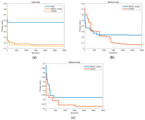
Figure 7.
Convergence results of particle swarm optimization (PSO), quantum-behaved particle swarm optimization (QPSO), and fuzzy-controlled quantum-behaved particle swarm optimization (FQPSO) algorithms in (a) light load, (b) medium load and (c) massive load.
Table 5.
The calculated results of minimal fitness by algorithms.
6.3. Evaluation of Incremental Scheduler
In our experiment, 100 problem instances are randomly generated for each dataset in Table 4. Each problem instance is optimized by FQPSO first. Then, an incremental scheduler for the frame instances is implemented based on the SMT in each basic period, and the average computation time is calculated. In order to evaluate the performance of each incremental scheduler under different priority ranking strategies, random ranking, period ascending, and proposed deadline-PU based priority are selected in this article. Table 6 shows the comparison of computation time. The upper limit of computation time for the SMT set in this article is 3600 s. If the result is not obtained within time limit, it will return “No solution” as unsolved.
Table 6.
Computation time with three ranking methods (in seconds).
The constraints given by Steiner in [28] are too many and complicated for the case of non-strictly periodic scheduling. It is very easy for the computation time to exceed the upper time limit and fail to obtain a feasible schedule. In this article, each frame instance is fixed in its own basic period by FQPSO, which can greatly reduce the searching space and number of constraints.
The experiment results in Table 6 show that the computation time of random frame ranking is significantly higher than that of the other two ranking methods due to no consideration of the schedulability of frames. For period ascending and deadline-PU priority ranking, when the problem scale is not large, the incremental scheduler performance is close. With the increase of time-triggered traffic in the network, the incremental scheduler based on the deadline-PU priority ranking has an obviously lower computation time compared with period ascending ranking, because the schedulability of a time-triggered frame depends not only on the period of the message, but also on the frame length, basic period length, and parameters of the other messages scheduled in the same basic period. These factors are comprehensively considered in the priority method proposed in this article and result in a more reasonable scheduling queue of frames.
6.4. Performance Results
After completing the FQPSO optimization and incremental scheduler, we perform scheduling performance analysis on all successful instances in the datasets. The incremental scheduler in [28] is used as a contrastive algorithm. Since the strictly periodic scheduling is used in these references, the collision-free constraint in [28] is changed as shown in Equation (19) to meet the requirements of non-strict periodic scheduling in this article. Delay and precedence can be constrained by Equations (4) and (5). The other assignments and constraints are the same as those in Section 6.1.
where L is the set of dataflow links, fi and fu are frames on lk, s(i,j,lk) and s(u,v,lk) are the sending offsets of their j-th and v-th instances, s(i,1,lk) and s(u,1,lk) are the sending offsets of the first instance of frame fi and fu on lk, and pi and pu are the link occupancy time of frames.
In two cases, the proposed approach may fail to provide solutions. Firstly, in level 1 of the proposed approach, FQPSO cannot get solutions satisfying the constraints in Equation (6). Secondly, in level 2, although the result of level 1 is satisfied, the collision-free problem cannot be solved, or the effective solution cannot be provided within the time limit by the incremental SMT scheduler due to the heavy network load.
Figure 8a shows the schedulability in the percentage of each dataset within the time limit of the standard incremental SMT [28] and FQPSO-SMT in this article. With non-strictly periodic frames, rapidly increasing the quantity of constraints makes it more difficult for the standard incremental SMT approach to find a feasible solution. The schedulability of our approach is always higher than that of standard incremental SMT and is always 100% when the dataflow link utilization is lower than 25%. No solution is obtained in the standard incremental SMT of datasets 7 and 8, while our approach achieves the schedulability of 39% and 26% within the time limit.
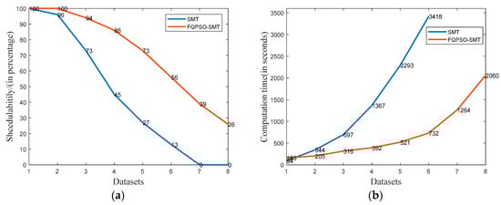
Figure 8.
(a) Schedulability of SMT and FQPSO-SMT algorithms. (b) Computation time of SMT and FQPSO-SMT algorithms.
Figure 8b shows the average computation time of standard incremental SMT and FQPSO-SMT in this article, and our approach always obtains a significantly lower result in all the datasets. On one hand, our FQPSO approach can optimize the QoS parameters of scheduling, such as macro period load balance, jitter, etc., at the cost of increasing computation time. On the other hand, our approach decreases the number of constraints by solving the problem in certain basic periods instead of the whole macro period, thus reducing the complexity and computation time. As a result, the standard incremental SMT computation time is slightly lower than that of FQPSO-SMT in the light load scenario of dataset 1 and is around 1.7 to 4.7 times that of datasets 2 to 6 in our testbench. The average computation time of our approach for dataset 7 and 8 is 1264 and 2060 s, while the results of incremental SMT are outside of the time limits.
For the link with the largest traffic load in every problem instance, we define the load balance as the standard deviation for basic period utilization as shown in Equation (3). The max frame jitter is divided by its message period as Jitteri/Ti. The experimental results are the average value of all the successful instances in each dataset. The statistics are shown in Table 7. If the result is not obtained within time limit of 3600 s, it will return “No solution” as unsolved.
Table 7.
Load balance and jitter results.
There are few research studies on jitter and load balance optimization of a basic period model for non-strictly periodic scheduling in switched Ethernet. We can only use the results of standard incremental SMT as a contrast and compare them with the results of proposed FQPSO-SMT approach in this article.
In Table 7, the load balance of FQPSO-SMT in all the test datasets is less than that of the contrast. The value obtained by FQPSO-SMT in dataset 8, which has the heaviest traffic, is 61.86 and less than the 63.64 obtained by incremental SMT in dataset 1, which has the smallest load. It proves that the FQPSO-SMT can make the schedule of time-triggered frames more balanced in the communication model based on a basic period structure. This balance optimization can improve the overall bandwidth utilization of the network. Furthermore, it provides more flexible time slots for the incremental scheduling of newly added network traffic.
The jitter in Table 7 deteriorates rapidly with the increase of traffic load without optimization. The optimized jitter of FQPSO-SMT is better than that of the contrast in all the datasets. When using the FQPSO-SMT algorithm, the increasing speed of jitter is significantly slower than that of the contrast algorithm, and the maximum frame jitter is less than half of its period. Therefore, our approach is more suitable for non-strictly periodic scheduling while the standard incremental SMT scheduler is only suitable for strictly periodic frames. In a train communication scenario, the time-triggered service generally does not exceed 50% of the total bandwidth, and the remaining bandwidth can be used by event-triggered and best effort traffic. The frame jitter at this point is less than 25% of its period as shown in dataset 5, which can meet the jitter requirements of train real-time services.
7. Conclusions
This article introduces a scheduling approach to design and optimize a time-triggered schedule table for non-periodic frames and tasks with hard real-time requirements that are executed on Ethernet in CPS. Our approach includes two levels: the optimization part in the first level and the incremental scheduler part in the second level. We present a co-scheduling model of load balance and frame jitter for the first level. Furthermore, an improved fuzzy-controlled QPSO method is proposed to realize the dynamic adaptive adjustment of CE coefficient and mutation rate in FQPSO and improve the algorithm performance when searching in a high-dimensional space. Based on these properties, an improved SMT incremental scheduler with a schedulability ranking method is proposed, which can fast solve the collision-free and temporal constraints of frames in basic periods. We evaluate the efficiency and performance of the proposed approach on the testbench of a train Ethernet network system with different traffic loads. The experiment demonstrates the effectiveness and scalability of our approach.
Our approach is an enhancement and improvement of a previous optimization algorithm and SMT solver scheduler. It is an exploration of NP-complete complexity mitigation for multitask scheduling optimization. This approach still has a few disadvantages. When the online incremental SMT scheduling of newly added traffic cannot succeed, the entire schedule table needs to be recalculated offline. A hierarchical submodel may be a solution and will be our future work. Another future work is the extension of the proposed approach to systems with mixed hardware properties, such as for example the Internet of Things, networks with different wire speeds, or wireless communication.
Author Contributions
Conceptualization, methodology, and writing—original draft preparation, J.J.; formal analysis, software, and programming, J.J. and H.C.; supervision, project administration, and writing—review and editing, L.W. and X.N. All authors have read and agreed to the published version of the manuscript.
Funding
This research was funded by Fundamental Research Funds for the Central Universities of China under Grant 2018YJS149, and the Natural Science Foundation of Beijing Municipality under Grant L171009.
Conflicts of Interest
The authors declare no conflict of interest.
References
- Rajkumar, R.; Lee, I.; Sha, L.; Stankovic, J. Cyber-physical systems: The next computing revolution. In Proceedings of the Design Automation Conference, Anaheim, CA, USA, 13–18 June 2010; pp. 731–736. [Google Scholar]
- Yu, X.F.; Tomsovic, K. Application of linear matrix inequalities for load frequency control with communication delays. IEEE Trans. Power Syst. 2004, 19, 1508–1515. [Google Scholar] [CrossRef]
- Bradley, J.M.; Atkins, E.M. Computational-Physical State Co-regulation in Cyber-Physical Systems. In Proceedings of the 2011 IEEE/ACM Second International Conference on Cyber-Physical Systems, Chicago, IL, USA, 12–14 April 2011; pp. 119–128. [Google Scholar]
- International Electrotechnical Commission. Industrial Communication Networks—Profiles—Part 1: Fieldbus Profiles. International Electrotechnical Commission 61784-1; International Electrotechnical Commission: Geneva, Switzerland, 2014. [Google Scholar]
- International Electrotechnical Commission. Industrial Communication Networks—Fieldbus Specifications—Part 2: Physical Layer specification and Service Definition, International Electrotechnical Commission 61158-2; International Electrotechnical Commission: Geneva, Switzerland, 2014. [Google Scholar]
- Beji, S.; Hamadou, S.; Gherbi, A.; Mullins, J. SMT-Based Cost Optimization Approach for the Integration of Avionic Functions in IMA and TTEthernet Architectures. In Proceedings of the 2014 IEEE/ACM 18th International Symposium on Distributed Simulation and Real Time Applications, Toulouse, France, 1–3 October 2014; pp. 165–174. [Google Scholar]
- Xue, Y.K.; Li, J.; Nazarian, S. Fundamental Challenges toward Making the IoT a Reachable Reality: A Model-Centric Investigation. ACM Trans. Des. Autom. Electron. Syst. (Todaes) 2017, 22, 1–25. [Google Scholar] [CrossRef]
- Derler, P.; Lee, E.A.; Vincentelli, A.S. Modeling Cyber–Physical Systems. Proc. IEEE 2012, 100, 13–28. [Google Scholar] [CrossRef]
- Poovendran, R. Cyber–Physical Systems: Close Encounters between Two Parallel Worlds [Point of View]. Proc. IEEE 2010, 98, 1363–1366. [Google Scholar] [CrossRef]
- Karsai, G.; Sztipanovits, K.; Ledeczi, A.; Bapty, T. Model-integrated development of embedded software. Proc. IEEE 2003, 91, 145–164. [Google Scholar] [CrossRef]
- Bogdan, P. A Cyber-Physical Systems Approach to Personalized Medicine: Challenges and Opportunities for NoC-based Multicore Platforms. In Proceedings of the 2015 Design, Automation & Test in Europe Conference & Exhibition (DATE), Grenoble, France, 9–13 March 2015; pp. 253–258. [Google Scholar]
- Alonso, J.M.; Ribas, J.; del Coz, J.J. Intelligent control system for fluorescent lighting based on LonWorks technology. In Proceedings of the 24th Annual Conference of the IEEE Industrial Electronics Society (Cat. No.98CH36200), Aachen, Germany, 31 August–4 September 1998; Volume 1, pp. 92–97. [Google Scholar]
- Liang, G.; Wang, H. Communication performance analysis and comparison of two patterns for data exchange between nodes in World FIP fieldbus network. ISA Trans. 2010, 49, 567–576. [Google Scholar] [CrossRef]
- Ferreira, J.; Almeida, L.; Fonseca, A.; Pedreiras, P.; Martins, E.; Rodriguez-Navas, G.; Rigo, J.; Proenza, J. Combining operational flexibility and dependability in FTT-CAN. IEEE Trans. Ind. Inform. 2006, 2, 95–102. [Google Scholar] [CrossRef]
- Pop, T.; Pop, P.; Eles, P.; Peng, Z.; Andrei, A. Timing analysis of the FlexRay communication protocol. In Proceedings of the 18th Euromicro Conference on Real-Time Systems (ECRTS’06), Dresden, Germany, 5–7 July 2006. [Google Scholar]
- Skeie, T.; Johannessen, S.; Brunner, C. Ethernet in substation automation. IEEE Control Syst. Mag. 2002, 22, 43–51. [Google Scholar]
- Skeie, T.; Johannessen, S.; Holmeide, O. Timeliness of real-time IP communication in switched industrial Ethernet networks. IEEE Trans. Ind. Inform. 2006, 2, 25–39. [Google Scholar] [CrossRef]
- IEEE Standard for Ethernet, IEEE 802.3; IEEE Standards Association: Piscataway, NJ, USA, 2015.
- Decotignie, J.D. Ethernet-Based Real-Time and Industrial Communications. Proc. IEEE 2005, 93, 1102–1117. [Google Scholar] [CrossRef]
- Bai, T.; Zhi-Ming, W.; Gen-Ke, Y. Optimal bandwidth scheduling of networked control systems (NCSs) in accordance with jitter. J. Zhejiang Univ.—Sci. A: Appl. Phys. Eng. 2005, 6, 535–542. [Google Scholar]
- Yan, X.; Li, H.-B.; Wang, L.; Shen, P. Optimal scheduling algorithm for reducing jitter in networked control systems based on estimation of distribution algorithms. J. Southeast Univ. Natrual Sci. Ed. 2013, 43, 38–43. [Google Scholar]
- Barreiros, J.; Costa, E.; Fonseca, J.; Coutinho, F. Jitter reduction in a real-time message transmission system using genetic algorithms. In Proceedings of the 2000 Congress on Evolutionary Computation, La Jolla, CA, USA, 16–19 July 2000; Volume 2, pp. 1095–1101. [Google Scholar]
- Natale, M.D.; Stankovic, J.A. Scheduling distributed real-time tasks with minimum jitter. IEEE Trans. Comput. 2000, 49, 303–316. [Google Scholar] [CrossRef]
- Xu, X.F.; Cao, C.; Guo, J.; Liu, Z. TT-RMS: Communication table generation algorithm of time-triggered network. J. Beijing Univ. Aeronaut. Astronaut. 2015, 41, 1403–1408. [Google Scholar]
- Zhang, C.; Nan, J.G.; Chu, W.K. An Improved Communication Table Generation Algorithm based on Time-Triggered Rate Monotonic Scheduling. J. Air Force Eng. Univ.: Nat. Sci. Ed. 2016, 17, 82–87. [Google Scholar]
- Tamas-Selicean, D.; Pop, P.; Steiner, W. Synthesis of communication schedules for TTEthernet-based mixed-criticality systems. In Proceedings of the 8th IEEE/ACM/IFIP International Conference on Hardware/software Codesign and System Synthesis, Tampere, Finland, 7–12 October 2012; pp. 473–482. [Google Scholar]
- Tamas-Selicean, D.; Pop, P.; Steiner, W. Design optimization of TTEthernet-based distributed real-time systems. Real-Time Syst. 2015, 51, 1–35. [Google Scholar] [CrossRef]
- Mok, A.; Rosier, L.; Tulchinsky, I.; Varvel, D. The pinwheel: A real-time scheduling problem. In Proceedings of the Twenty-Second Annual Hawaii International Conference on System Sciences, Kailua-Kona, HI, USA, 3–6 January 1989; Volume II: Software Track, pp. 693–702. [Google Scholar]
- Hanzalek, Z.; Burget, P.; Sucha, P. Profinet IO IRT Message Scheduling with Temporal Constraints. IEEE Trans. Ind. Inform. 2010, 6, 369–380. [Google Scholar] [CrossRef]
- Steiner, W. An Evaluation of SMT-Based Schedule Synthesis for Time-Triggered Multi-hop Networks. In Proceedings of the 31st IEEE Real-Time Systems Symposium, San Diego, CA, USA, 30 November–3 December 2010; pp. 375–384. [Google Scholar]
- Pozo, F.; Rodriguez-Navas, G.; Hansson, H.; Steiner, W. SMT-based synthesis of TTEthernet schedules: A performance study. In Proceedings of the 10th IEEE International Symposium on Industrial Embedded Systems (SIES), Siegen, Germany, 8–10 June 2015; pp. 1–4. [Google Scholar]
- Huang, J.; Blech, J.O.; Raabe, A.; Buckl, C.; Knoll, A. Static scheduling of a Time-Triggered Network-on-Chip based on SMT solving. In Proceedings of the 2012 Design, Automation & Test in Europe Conference & Exhibition (DATE), Dresden, Germany, 12–16 March 2012; pp. 509–514. [Google Scholar]
- Craciunas, S.S.; Oliver, R.S. Combined task and network-level scheduling for distributed time-triggered systems. Real-Time Syst. 2015, 52, 161–200. [Google Scholar] [CrossRef]
- Minaeva, A.; Akesson, B.; Hanzálek, Z.; Dasari, D. Time-Triggered Co-Scheduling of Computation and Communication with Jitter Requirements. IEEE Trans. Comput. 2018, 67, 115–129. [Google Scholar] [CrossRef]
- Wang, N.; Yu, Q.; Wan, H.; Song, X.; Zhao, X. Adaptive Scheduling for Multicluster Time-Triggered Train Communication Networks. IEEE Trans. Ind. Inform. 2019, 15, 1120–1130. [Google Scholar] [CrossRef]
- Syed, A.; Fohler, G. Efficient offline scheduling of task-sets with complex constraints on large distributed time-triggered systems. Real-Time Syst. 2019, 55, 209–247. [Google Scholar] [CrossRef]
- Sun, J.; Fang, W.; Wu, X.; Palade, V.; Xu, W. Quantum-Behaved Particle Swarm Optimization: Analysis of Individual Particle Behavior and Parameter Selection. Evol. Comput. 2012, 20, 349–393. [Google Scholar] [CrossRef] [PubMed]
- Huang, W.; Xu, X.; Pan, X. Control strategy of contraction-expansion coefficient in quantum-behaved particle swarm optimization. Appl. Res. Comput. 2013, 30, 1967–1970. [Google Scholar]
- Liu, P.; Leng, W.; Fang, W. Training ANFIS Model with an Improved Quantum-Behaved Particle Swarm Optimization Algorithm. Math. Probl. Eng. 2013, 2013, 595639. [Google Scholar] [CrossRef]
- Yadmellat, P.; Salehizadeh, S.M.A.; Menhaj, M.B. A New Fuzzy Inertia Weight Particle Swarm Optimization. In Proceedings of the 2009 International Conference on Computational Intelligence and Natural Computing, Wuhan, China, 6–7 June 2009; pp. 507–510. [Google Scholar]
- Wang, Y.; Wang, L.; Yan, X.; Shen, P. Fuzzy immune particle swarm optimization algorithm and its application in scheduling of MVB periodic information. J. Intell. Fuzzy Syst. 2017, 32, 3797–3807. [Google Scholar] [CrossRef]
- Xu, B.; Zhang, X.; Liu, L. The Failure Detection Method of WSN Based on PCA-BDA and Fuzzy Neural Network. Wirel. Pers. Commun. 2018, 102, 1657–1667. [Google Scholar] [CrossRef]
- Roman, R.C.; Precup, R.E.; Petriu, E.M. Model-free adaptive control with fuzzy component for tower crane systems. In Proceedings of the 2019 IEEE International Conference on Systems, Man, and Cybernetics (SMC), Bari, Italy, 6–9 October 2019; pp. 1–6. [Google Scholar]
- Roman, R.C.; Precup, R.E.; Bojan-Dragos, C.A. Combined Model-Free Adaptive Control with Fuzzy Component by Virtual Reference Feedback Tuning for Tower Crane Systems. Procedia Comput. Sci. 2019, 162, 267–274. [Google Scholar] [CrossRef]
- International Electrotechnical Commission. Electronic Railway Equipment—Train Communication Network (TCN)—Part 3-4: Ethernet Consist Network (ECN), International Electrotechnical Commission 61375-3-4; International Electrotechnical Commission: Geneva, Switzerland, 2014. [Google Scholar]
- International Electrotechnical Commission. Electronic Railway Equipment—Train Communication Network (TCN)—Part 2-3: TCN Communication Profile, International Electrotechnical Commission 61375-2-3; International Electrotechnical Commission: Geneva, Switzerland, 2015. [Google Scholar]


© 2020 by the authors. Licensee MDPI, Basel, Switzerland. This article is an open access article distributed under the terms and conditions of the Creative Commons Attribution (CC BY) license (http://creativecommons.org/licenses/by/4.0/).