Determining an Appropriate Parameter of Analytical Wake Models for Energy Capture and Layout Optimization on Wind Farms

Abstract

The wake of a wind turbine is a crucial factor that decreases the output of downstream wind turbines and causes unsteady loading. Various wake models have been developed to understand it, ranging from simple ones to elaborate models that require long calculation times. However, selecting an appropriate wake model is difficult because each model has its advantages and disadvantages as well as distinct characteristics. Furthermore, determining the parameters of a given wake model is crucial because this affects the calculation results. In this study, a method was introduced of using the turbulence intensity, which can be measured onsite, to objectively define parameters that were previously set according to the subjective judgement of a wind farm designer or general recommended values. To reflect the environmental effects around a site, the turbulence intensity in each direction of the wind farm was considered for four types of analytical wake models: the Jensen, Frandsen, Larsen, and Jensen–Gaussian models. The prediction performances of the wake models for the power deficit and energy production of the wind turbines were compared to data collected from a wind farm. The results showed that the Jensen and Jensen–Gaussian models agreed more with the power deficit distribution of the downstream wind turbines than when the same general recommended parameters were applied in all directions. When applied to energy production, the maximum difference among the wake models was approximately 3%. Every wake model clearly showed the relative wake loss tendency of each wind turbine.

1. Introduction

In a wind farm, wind turbines exchange wake effects with each another. This causes wake loss, where the wake of a wind turbine decreases the power of turbines located downstream. This wake loss is inevitable in a wind farm, and many studies have focused on minimizing wake effects to optimize the wind farm layout [1,2]. Various optimization algorithms have been developed, including wake models that calculate the wind speed deficit according to the wake. The main focuses of wake models are the wind speed deficit, which affects the downstream wind turbine power, and turbulence, which adds an unstable load. The former affects the prediction of the energy production by a wind farm and thus can be used to optimize a wind farm layout.

Understanding the form and state of the wake generated by wind turbines is difficult because of the complex mechanism and nonlinear phenomena inside the wake [3]. Research has been ongoing to develop various wake models, from simple ones to elaborate models with high computational costs. For these efforts to succeed, the wake effect in a wind farm needs to be understood correctly.

Wake models can be categorized as analytical or numerical; these are also known as kinematic and field models, respectively. Analytical models provide an analytical solution and can calculate the wind speed deficit from the wake via an induced formula, whereas numerical models calculate the wake flow field numerically based on the Navier–Stokes (NS) equation.

The first useful analytical model was introduced by Lissaman [4] in 1979 in relation to the development of the blade element theory and momentum theory. Since then, wake models based on the momentum theory have been developed. The most representative and widely used analytical model is the Jensen model [5], which was further developed by Katic et al. [6]. It can calculate the wind speed deficit due to a wake under the assumption that the wake diameter increases linearly in proportion to the downstream distance and the wind speed distribution in the radial direction of the wake is identical. The Jensen model is simple but shows useful results in the far-wake area. It is included as the basic model in many commercial software applications, and many derivative wake models have been developed [7,8,9,10,11]. Frandsen et al. [12] proposed a wake model for predicting the wind speed deficit in an offshore wind farm where wind turbines are equally spaced and arranged in a grid form. Larsen [13,14] developed a wake model that approximates the NS equation, which is the governing equation of numerical models and cannot normally be solved by an analytical method. However, Larsen simplified it by assuming the incompressible and inviscid condition and presented a closed-form solution by further reducing the dimensions based on the assumption that the wake deficit is axisymmetric.

Gaussian-based models are derived from the Jensen model and complement the radial wind speed distribution, which cannot be expressed by the Jensen model, by assuming that the radial wind speed follows a Gaussian distribution. Gao et al. [8] derived a two-dimensional wake model equation by using the Gaussian function. Sun and Yang [9], Xie and Archer [10], and Bastankhah and Porté-Agel [11] presented three-dimensional wake model equations that consider the wind profile in the height direction.

Numerical models are based on the NS equation with a turbulence model for closure. These can be classified into models based on the Reynolds-averaged Navier–Stokes (RANS) equations and models based on the large eddy simulation (LES). The first numerical model was developed in 1988by Ainslie [15], who used an incompressible NS equation with eddy viscosity (EV) closure. This wake model is also known as the EV model. Since the Ainslie model was introduced, commercial wake models that complement it have been developed (e.g., DAWM in OpenWIND, LAWF in Wind farmer) [16]. To overcome the enormous calculation time of the RANS-based numerical model, Ott et al. [17] developed the Fuga model, which is a linearized RANS model. This model can generate an error related to momentum balance due to linearization but showed good agreement with the observation results for the Horns Rev 1 and Nysted offshore wind farms. Larsen suggested the dynamic wake meandering (DWM) model, which describes the wake as a passive tracer driven by large-scale turbulence structures in the atmospheric boundary layer [18,19]. LES [20,21,22] is a powerful technique that can simulate the interaction between a turbine and surrounding air. In contrast to RANS-based models, which generally calculate in the steady state, LES describes the unsteady state. However, these advantages require numerous computational costs to calculate the wake field. Thus, LES is not appropriate for calculating the energy production of a wind farm, which requires calculating the power production in various wind directions and speeds [17,23].

Numerical wake models can be helpful for detailed research on the interaction between turbulence and the rotor blade or the interaction between wakes, but it seems less effective than analytical wake models in terms of estimating the annual energy production (AEP) of the entire wind farm considering wake loss. The rapid advances in computer hardware should help address this problem, but numerical models are also becoming sophisticated. Hence, it will not be easy to dramatically decrease the calculation time of numerical wake models in the near future. Therefore, this study compared and evaluated analytical wake models, which can easily calculate the wind farm energy production and be applied to optimizing the wind farm layout.

Comparative studies on wake models can be found in the existing literature. In 2005, Barthelmie et al. [24] compared the calculation results of six wake models (Risø engineering, Risø analytical, Risø WAsP, UO FLaP, ECN Wakefarm, and RGU CFD) developed by different European institutions that participated in the Efficient Development of Offshore Wind farms (ENDOW) project based on wind speed profiles measured with SODAR (sonic detecting and ranging) at an offshore wind farm. However, they did not present a specific wake model with excellent performance. In 2011, the UpWind project of the European Union compared the power deficits of wind turbines due to wakes at an offshore wind farm (Horns Rev and Nysted) using more diverse wake models (WAsP, Windfarmer, Canopy, Wakefarm, CFDWake, FlowNS, NTUA) [25,26,27]. The comparison of the power deficit results revealed that the WAsP model, which was based on the Jensen model, tended to underestimate the deficit compared to other models. Beaucage et al. [23] compared six commercial and research wake models (Park, EV, DAWM, Fuga, WindModeller, ARPS) and reported that the Park model based on the Jensen and EV models underestimated the wake loss. Tong et al. [28] compared energy production with no measurements among four analytical wake models (Jensen, Frandsen, Larsen, and Ishihara). Brusca et al. [29] performed wind tunnel experiments to obtain the wind speed deficits with three analytical wake models (Jensen, Frandsen, and Larsen) and reported that the Larsen model showed the highest matching rate, but they did not present the parameters applied to the wake models. Göçmen et al. [30] compared analytical models (Jensen, Larsen) and numerical models (DWM, Fuga, Ellipsys3D LES and RANS) with data collected from onshore (Sexbierum) and offshore (Lillgrund) wind farms. They argued that analytical models are convenient for application to large wind farms, whereas the numerical models matched well with the measurements but have very limited applicability to large wind farms because of the long calculation time. Archer et al. [31] compared the power deficits for offshore wind turbines with a regular layout (Lillgrund), offshore wind turbines with an irregular layout (Anholt), and onshore wind turbines with a regular layout (Nørrekær) using six analytical models (Jensen, Larsen, Frandsen, XA, BPA, and GM). They found that the Jensen and XA (Gaussian-based) models showed excellent results and recommended the Jensen and Frandsen models for wind farm layout optimization.

The dominant opinion of the above studies was that numerical models have higher accuracy than analytical models, but their calculation cost is too high for application to large wind farms. Analytical wake models may or may not match well depending on the wind direction at different sites or even within the same site, and the evaluation of the same wake model also differed from study to study. This seems to be because the generally recommended values were applied to the wake model parameters, which affect the calculation results. For example, in the Jensen model, a wake decay constant (WDC) of 0.04 for offshore and 0.075 for onshore is generally used in many studies. This means that the model assumes the same environment for all sites, but the environmental characteristics of each site may vary from region to region; even within one site, the environment may differ depending on the direction and surrounding environment. In this study, a method was introduced of using the turbulence intensity (TI), which can be measured at the site, in order to objectively define parameter values of a wake model that were previously set according to the analyst’s judgment or recommended values. To reflect the environmental impact around a site, the results of four analytical wake models (Jensen, Frandsen, Larsen, and Gaussian-based) were compared when the turbulence intensity according to the wind direction was considered.

The remainder of the paper is organized as follows. Section 2 introduces the analytical wake models. Section 3 compares the power deficits of the wind turbines and energy losses of the wind farm according to collected data with the wake model calculations. Finally, Section 4 presents the conclusions.

2. Wake Models

2.1. Jensen Wake Model

The Jensen wake model was first proposed by Jensen in 1983 [5] and modified by Katic et al. in 1986 [6]; it is a representative wake model that is still widely used. It is known to only be valid in the far-wake region because of its simple assumptions [2]. The near-wake region, where the geometry of the wind turbine directly affects the wake, has been reported to extend approximately 2–3D (where D is the rotor diameter) downstream of the wind turbine [32]. Schepers [33] suggested that the near-wake distance is 2.25D downstream of the wind turbine based on the ENDOW project. Hence, there is no problem with applying the model to a wind farm because the minimum distance between wind turbines is generally 3D. Therefore, many studies on wind turbine layouts use the Jensen model owing to its simple equation and easy applicability.

The wind speed deficit (δU) in the wake and the extended wake diameter (D_w) are expressed as follows:

$$\delta U(x)=U_0\left(1-\sqrt{1-C_t}\right){\left(\frac{D_0}{D_w}\right)}^2,$$

(1)

$$D_w=D_0+2k_{w}x,$$

(2)

where x is a downstream distance of the wake, U₀ is free stream wind speed, C_t is the thrust coefficient, D₀ is the rotor diameter of the upstream wind turbine, and k_w is the wake decay constant.

2.2. Frandsen Wake Model

The Frandsen model [12] was proposed by Frandsen in 2006 and applies the momentum theory while assuming self-similarity. It also assumes a constant wind speed distribution in the radial distance of the wake like the Jensen model. It differs because it considers the wake diameter that is initially extended at the rotor of the wind turbine, and the wake diameter downstream of the wind turbine is extended in the square root shape (k = 2) or Schlichting solution (k = 3) [34].

In the Frandsen model, the wind speed deficit and wake expansion diameter are expressed as follows:

$$\delta U(x)=\frac{U_0}{2}\left(1-\sqrt{1\hspace{0.17em}-\hspace{0.17em}2\frac{A_0}{A_w}\hspace{0.17em}{C}_t}\right),$$

(3)

$$D_w=D_0{\left({\beta }^{k/2}+\alpha s\right)}^{1/k},$$

(4)

$$\beta =\frac{1\hspace{0.17em}+\hspace{0.17em}\sqrt{1\hspace{0.17em}\hspace{0.17em}-\hspace{0.17em}\hspace{0.17em}{C}_t}}{2\hspace{0.17em}\sqrt{1\hspace{0.17em}\hspace{0.17em}-\hspace{0.17em}\hspace{0.17em}{C}_t}}\hspace{0.17em},\hspace{0.17em}\hspace{0.17em}\hspace{0.17em}s=x/D_0,$$

(5)

where A₀ = (πD₀²)/4 is the rotor swept area of the upstream wind turbine, A_w = (πD_w²)/4 is the expanded area of the wake and α is the wake decay factor of the Frandsen model and can be calculated with Equation (2) for the wake diameter in the Jensen model as follows:

$$\alpha ={\beta }^{k/2}\hspace{0.17em}\left[{\left(1+2\hspace{0.17em}\hspace{0.17em}{k}_w\hspace{0.17em}s\right)}^k\hspace{0.17em}\hspace{0.17em}-\hspace{0.17em}\hspace{0.17em}1\right]\hspace{0.17em}\hspace{0.17em}{s}^{-1}.$$

(6)

2.3. Larsen Wake Model

The Larsen model [13] was proposed by Larsen in 1988 and is also known as the EWTS II model. It was derived based on the thin shear layer approximation for the NS equation. By assuming non-viscosity, incompressibility, and similarity, Larsen derived the first- and second-order solutions for the ordinary differential equation. He considered the first-order model to be of practical importance for approximating the characteristics of the stationary wake deficit [14]. The present study also used the first-order model.

The wind speed deficit is a function of the axial distance x in the Jensen model; in the Larsen model, it is a function of the axial distance x and radial distance r:

$$\delta U(x,r)=-\frac{U_0}{9}{\left[C_t{A}_0{(x+x_0)}^{-2}\right]}^{1/3}{\left\{r^{3/2}{\left[3c_1{}^2{C}_t{A}_0(x+x_0)\right]}^{-1/2}-{\left(\frac{35}{2\pi }\right)}^{3/10}{(3c_1{}^2)}^{-1/5}\right\}}^2,$$

(7)

$$D_w=2{\left(\frac{105c_1^2}{2\pi }\right)}^{1/5}{\left[C_t{A}_0(x+x_0)\right]}^{1/3},$$

(8)

where c₁ denotes the non-dimensional turbulent mixing length, which is related to Prandtl’s mixing length. x₀ denotes the relative position of the rotor in the applied coordinate system and is expressed as follows:

$$c_1={\left(\frac{\sqrt{\beta }{D}_0}{2}\right)}^{5/2}{\left(\frac{105}{2\pi }\right)}^{-1/2}{(C_t{A}_0{x}_0)}^{-5/6},$$

(9)

$$x_0=\frac{9.6D_0}{{\left(\frac{2R_{9.6}}{\sqrt{\beta }{D}_0}\right)}^3-1}.$$

(10)

R_9.6 is the wake radius at the wind turbine downstream distance of 9.6D. It was experimentally determined as follows:

$$R_{9.6}=a_1\exp (a_2{C}_t^2+a_3{C}_t+a_4)(b_1{I}_a+1)D_0,$$

(11)

where a₁ = 0.435449861, a₂ = 0.797853685, a₃ = −0.124807893, a₄ = 0.136821858, and b₁ = 15.6298.

2.4. Jensen–Gaussian Wake Model

The Jensen–Gaussian model was recently proposed by Gao et al. [8] and can calculate the wind speed distribution in the radial direction inside the wake, which cannot be expressed by the Jensen model. Gao et al. reorganized the Jensen model by assuming the wake radial wind speed to have a Gaussian distribution. It was adopted for comparison with the traditional axisymmetric wake models given above.

In the Jensen–Gaussian model, the wind speed deficit according to the axial distance and radial direction are as follows:

$$\{\begin{array}{l}\delta U(x)=U_0\left(1-\sqrt{\hspace{0.17em}1-C_t}\right){\left(\frac{D_0}{D_w}\right)}^2\\ \delta U(x,r)=\delta U(x)\frac{5.16}{\sqrt{2\pi }}\exp \left(\frac{-r^2}{2{(R_w/2.58)}^2}\right)\end{array},$$

(12)

$$D_w=D_0+2\hspace{0.17em}{k}_{wake}\hspace{0.17em}x,$$

(13)

where k_wake is a new wake decay constant that replaces the wake decay constant k_w of the Jensen model. Although it has a similar function of being involved in the wake extension diameter, this parameter is calculated by considering the ambient turbulence intensity (I_a) and turbine-induced turbulence of the site:

$$k_{wake}=k_w\frac{I_{eff}}{I_a},$$

(14)

$$I_{eff}={\left(\frac{0.4C_t}{{(x/D_0)}^{0.5}}+I_a^{0.5}\right)}^2.$$

(15)

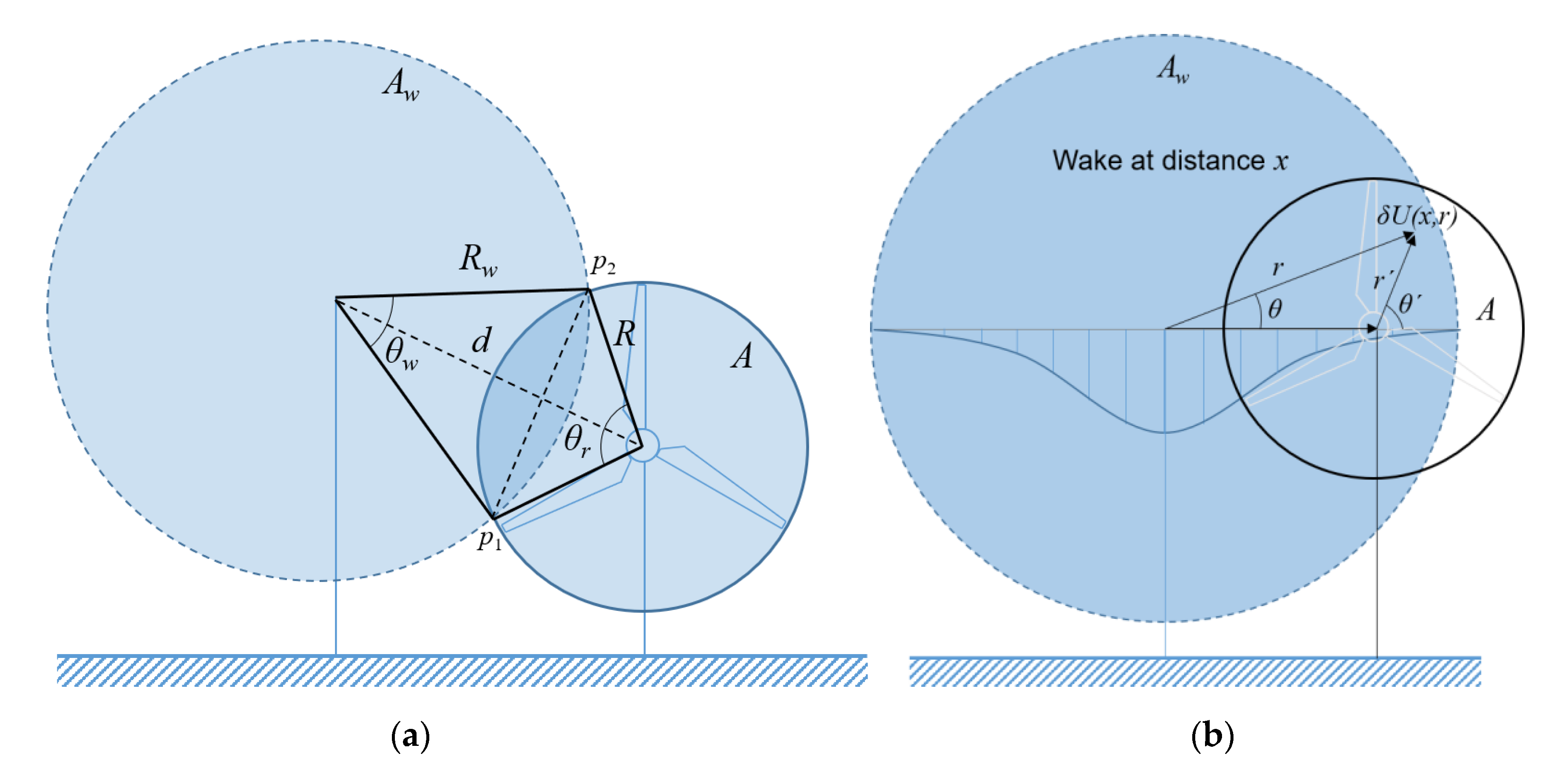
2.5. Partial and Multiple Wakes

To calculate the wind turbine power deficit due to the wake, the average wind speed deficit in the turbine rotor area subject to the wake effect needs to be known. The rotor of the wind turbine affected by the wake is fully or partially affected by the wake depending on the wind direction. The Jensen and Frandsen models assume that the wind speed in the rotor radial direction is constant. Hence, the wind speed deficit at the distance x is the mean wind speed deficit. This is the case when the wind turbine is fully in the wake. If it is partially affected, it can be calculated as the ratio of the intersecting area between the wake and rotor to the rotor area:

$$\delta \overline{U}=\delta U(x)\frac{A_{overlap}}{A},$$

(16)

where A_overlap is the intersecting area of the wake and wind turbine and A is the rotor swept area of the downstream wind turbine. A_overlap can be calculated as follows from the area of the fan shape created by connection of the centers of the wake and rotor with the intersection points (p₁, p₂) of the two circles and the triangle that connects the intersection points, as shown in Figure 1a [35]:

$$A_{partial}=\frac{1}{2}\left[R_w^2({\theta }_w-\sin {\theta }_w)+R_r^2({\theta }_r-\sin {\theta }_r)\right],$$

(17)

$${\theta }_w=2{\cos }^{-1}\left(\frac{d^2+(R_w^2-R_r^2)}{2d{R}_w}\right),$$

(18)

$${\theta }_r=2{\cos }^{-1}\left(\frac{d^2-(R_w^2-R_r^2)}{2d{R}_r}\right).$$

(19)

In the Larsen and Jensen–Gaussian models, the wind speed deficit changes with the axial and radial directions of the wake. Hence, the mean wind speed deficit ($\delta \overline{U}$) acting on the rotor area subject to the wake effect can be calculated by integrating the deficit at every location (r′, θ′) in the rotor area [36]:

$$\delta \overline{U}=\frac{{\displaystyle {\int }_A\delta U(x,r)dA}}{A}=\frac{1}{\pi R^2}{\displaystyle {\int }_{{\theta }^{\prime }=0}^{{\theta }^{\prime }=2\pi }{\displaystyle {\int }_{r^{\prime }=0}^{r^{\prime }=R}\delta U(x,r)r^{\prime }d{r}^{\prime }d{\theta }^{\prime }}},$$

(20)

where r′ and θ′ are the variables of the local polar coordinates of the wind turbine rotor affected by the wake effect, as shown in Figure 1b. This can be used to obtain the internal wind speed deficit δU(x, r), which changes at a random position of the rotor, through coordinate conversion to global polar coordinates (r, θ) based on the wake.

Wind turbines in a wind farm can be affected by the wakes generated by upstream wind turbines simultaneously depending on the wind direction. To calculate the wind speed deficit by these multiple wakes, the different superposition methods are available: linear superposition of velocity deficit or energy deficit [37]. In this study the following method based on the conservation of kinetic energy is adopted. This model assumes that the kinetic energy deficit by mixed wakes is equal to the sum of the kinetic energy deficits by each wake.

The mean wind speed deficit of wind turbine j due to the wakes generated by N wind turbines i can be expressed as follows:

$$\delta {\overline{U}}_j=\sqrt{{\displaystyle \sum _{i=1}^N\delta {\overline{U}}_i^2}}.$$

(21)

2.6. Wake Model Parameters

The most important and difficult problem with using wake models is determining appropriate values for the parameters of each wake model at a site. Furthermore, each wake model uses different types of parameters. The Jensen and Frandsen models must determine the WDC k_w; the Larsen model must determine the ambient turbulence intensity I_a; and the Jensen–Gaussian model must determine the two parameters of the WDC and ambient turbulence intensity.

To determine the WDC, the following equation is generally calculated by using the surface roughness length of the site, which depends on the judgment of the wind farm designer: k_w = 0.5/ln(z/z₀). However, because subjective judgement is required, many studies use the recommended values (offshore = 0.04, onshore = 0.075) in the literature. This means that every wind farm is treated as being in the same environment when each wind farm actually has a different environment. Furthermore, like the Larson model, similarities among parameters (e.g., WDC and TI) need to be found in order to compare wake models with different types of parameters.

Crespo and Hernández [38] stated that turbulence is a major physical property in a far-wake region. Peña et al. [39] reported that the WDC is related to the height, roughness, and atmospheric stability and is ultimately correlated with the turbulence intensity. They proposed the following equation for estimating the WDC from the relationship between the turbulence intensity and atmospheric stability based on the boundary layer theory:

$$\mathrm{TI}\approx {\left[\ln \left(\frac{z}{z_0}\right)-{\psi }_m(z/L)\right]}^{-1},$$

(22)

$$k_w\approx 0.4{\mathrm{TI}}_h,$$

(23)

where ψ_m(z/L) is the local atmospheric stability correction and TI_h is the hub height TI.

To compare the performances of wake models, they must satisfy equivalent conditions. When Equation (23) is used, the above wake models have one major parameter of turbulence intensity; thus, they have consistency. The ambient turbulence intensity that reflects a site’s characteristics can be obtained from wind condition data measured by a meteorological mast at the site.

3. Wake Model Comparison for an Onshore Wind Farm

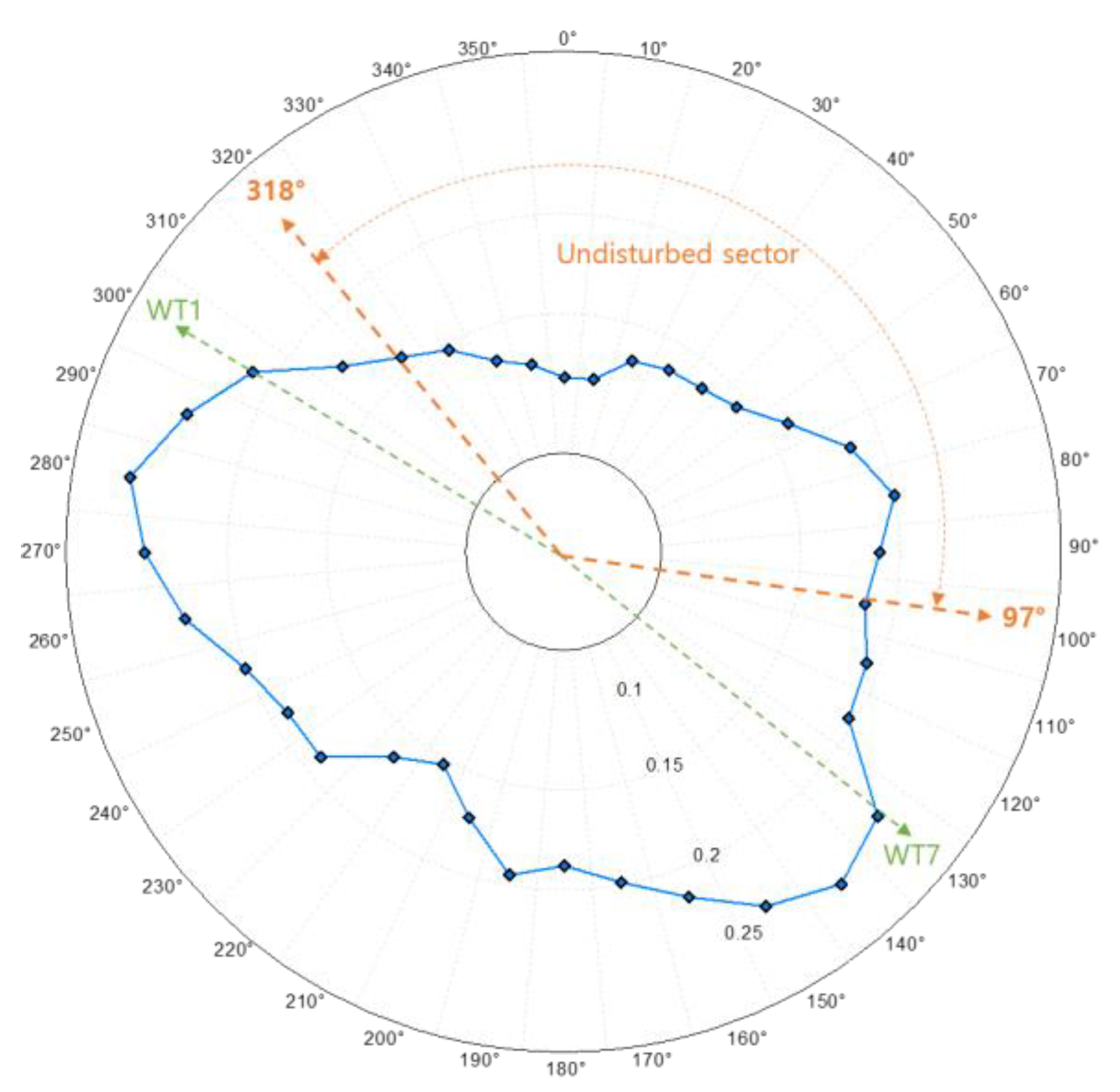
3.1. Wind Farm Layout

To evaluate the performances of the wake models, the power deficits due to wakes were compared according to wind turbine SCADA (supervisory control and data acquisition) data collected from an onshore wind farm in operation and wind data collected from a meteorological mast near the wind farm. Figure 2 shows the layout of the Gasiri wind farm from which the SCADA data were collected. The Gasiri wind farm operates on Jeju Island, which is south of the Korean peninsula. Jeju Island has wind resources appropriate for a wind farm, and approximately 10 onshore and offshore wind farms generating 20–30 MW are in operation. The Gasiri wind farm consists of six 660 kW wind turbines (WT1–6) and seven 1500 kW wind turbines (WT7–13), as shown in Figure 2. The wind turbines are arranged in a grid form in the direction of the prevailing winds.

The wind turbines selected for the wake models were WT7–WT10 and WT7–WT9, which are shown in Figure 2. They were determined by considering the state of the collected data and interference between wind turbines within the measurement range.

Table 1. Wind turbine specifications.

Specification	Value
Rated power [kW]	1500
Hub height [m]	70
Rotor diameter [m]	77
Cut-in wind speed [m/s]	3.5
Rated wind speed [m/s]	13
Cut-out wind speed [m/s]	25

presents the specifications of the wind turbines used for analysis. The distances between wind turbines were 3.8D (WT7–WT10) or 4.9D (WT7–WT9). For the analysis of the data collected from wind turbine pairs and the wake model calculations, the actual average power data in the range where downstream turbines are affected by the wake according to the wind direction were calculated. The wake model calculations in the same direction were compared, as shown in Figure 3.

The data collected from the meteorological mast were used for the free stream wind speed. For the wake analysis, only the data of wind turbines operating simultaneously were synchronized and analyzed. This process is essential because wind turbines can have different operating situations (e.g., maintenance, wind turbine errors). For the wake model calculation, each wake model was coded with the C++ language, and the wind speed distribution inside the wake was simulated to calculate the wake effect on the power.

Figure 4 shows the distribution of the turbulence intensity in each direction for the Gasiri wind farm and the range of wind directions applied to the analysis. To determine the parameters of the wake models described in Section 2.6, the turbulence intensity was calculated in each direction using the data collected from the meteorological mast. However, the mast was affected by the wind turbines depending on the wind direction. Thus, the undisturbed sector that was not affected by the surrounding turbines was calculated by using the obstacle evaluation method from the IEC 61400-12-1 standard and was applied as the range. The WT7–WT10 and WT7–WT9 pairs used in the analysis were within the undisturbed sector.

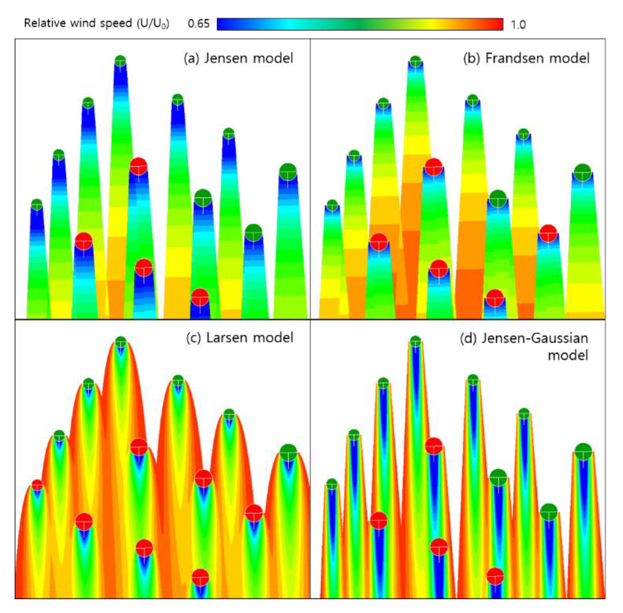
3.2. Wind Speed Deficit Comparison

The basic characteristics of each wake model were analyzed first before the power deficits due to wakes were compared. The wake models were compared for the wind speed deficit with no measured data. Figure 5a compares the wind speed deficits for the radial wind speed distribution according to the four wake models at a downstream distance of 3.8D and wind speed of 8 m/s (WT7–WT10). A turbulence intensity of 0.14 was applied to the calculation, which corresponds to k_w = 0.056 when converted to the WDC. For the Jensen and Frandsen models, the wind speed deficit was constant. For the Larsen and Jensen–Gaussian models, the wind speed graph showed a bell shape, where the wind speed deficit was largest at the center of the wake and then decreased gradually. The Jensen–Gaussian model showed the wind speed deficit as a typical Gaussian distribution. The Larsen model showed a low wind speed deficit and a broad wind speed distribution. In other words, the Larsen model predicted a broader range of wake diameters than the other models. The Frandsen model calculated the lowest wake deficit and had a larger wake diameter than the Jensen model. This is because the Frandsen model considers the initial wake extension diameter at the turbine position.

Figure 5b compares the wind speed deficit at the wake center according to the downstream distance. The wind speed gradually recovered downstream of the wake. The Jensen–Gaussian model predicted the largest wind speed deficit according to the distance, and the Frandsen model predicted the lowest wind speed deficit among the four models. The next section discusses the accuracy of the four models when compared with the measured power data.

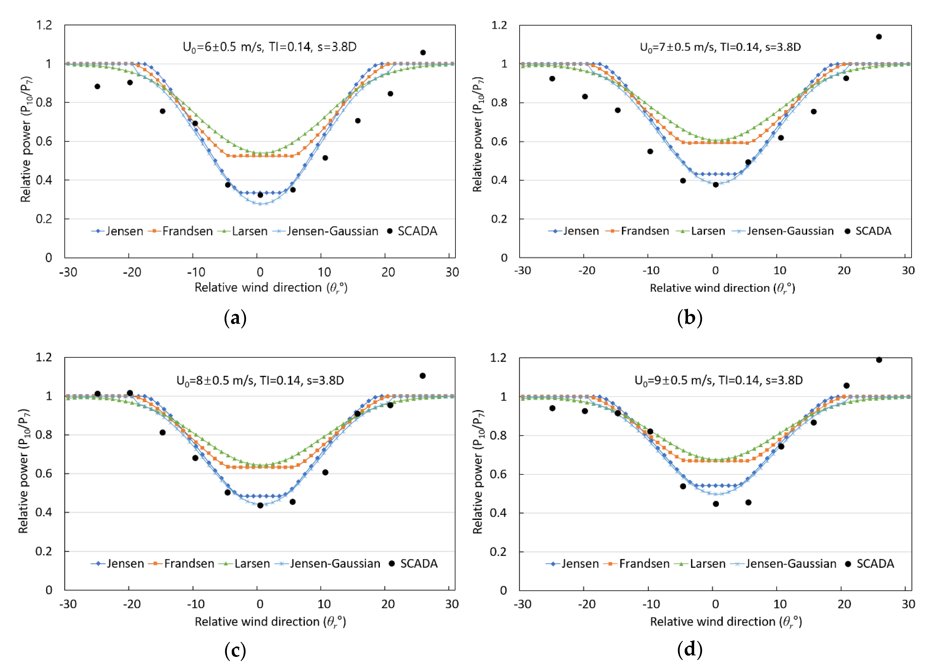
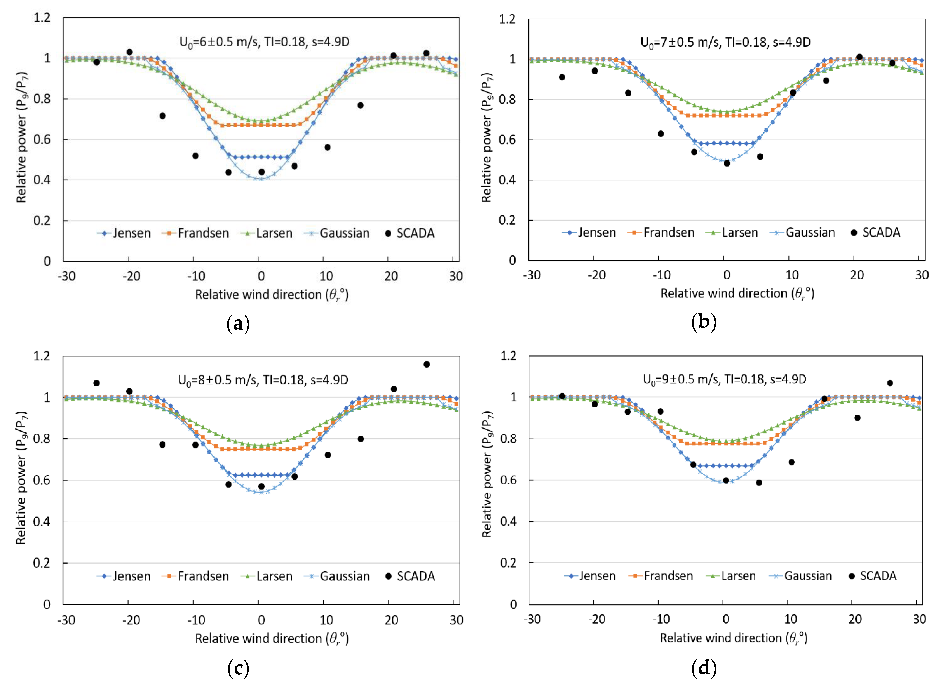
3.3. Power Deficit Comparison

To verify the performances of the wake models, the power deficits due to wakes were compared for the above wind turbine pairs of the Gasiri wind farm. The relative power of two turbines was compared with SCADA data collected at intervals of 1 ± 0.5 m/s in the wind speed section of 6–9 m/s. Data provided by the manufacturer were used to set the thrust coefficient required for calculating the wake models and the power curve required for calculating the wind turbine power.

Figure 6 compares the relative power (P₁₀/P₇) data (

Table 2. Power deficit ratios (%) of SCADA due to wakes at 3.8D.

θr°	−25	−20	−15	−10	−5	0	5	10	15	20	25
6 m/s	11.7	9.6	24.4	30.6	62.3	67.6	64.8	48.5	29.2	15.4	−5.8
7 m/s	7.5	16.8	23.9	45.0	60.1	62.2	50.6	38.1	24.5	7.4	−14.1
8 m/s	−1.4	−1.7	18.6	31.7	49.6	56.2	54.4	39.2	9.1	4.6	−10.6
9 m/s	5.8	7.4	8.4	17.9	46.1	55.2	54.5	25.6	13.2	−5.8	−19.2

) collected at a distance of 3.8D between the WT7 and WT10 turbines and the calculation results using the four wake models according to wind speed. The wind direction was θ_a = 30°, and the turbulence intensity in this direction was TI = 0.14 (k_w = 0.056 when converted to the WDC). In general, the relative power decreased as the wind speed increased. This is related to the thrust coefficient of a wind turbine, which decreases with an increasing wind speed. Depending on the wind speed, the power of the wind turbine (WT10) affected by the wake decreased about 67% at 6 m/s and decreased about 55% at 9 m/s compared to the upstream wind turbine. Of course, because more power is generated at higher wind speeds, the amount of energy reduction increased with the wind speed.

Among the four wake models, the Jensen–Gaussian model agreed well with the SCADA data at every wind speed. The Jensen model also showed good agreement. However, the Frandsen and Larsen models underestimated the power deficit. The Larsen model predicted the actual wake diameter better because the range of the power deficit according to the wind direction was similar to that in the SCADA data. The Larsen model calculated a lower power deficit than the Frandsen model, but the Frandsen model calculated a lower wind speed deficit. This is because the Larsen model uses a bell-shaped wind speed distribution, so it uses a lower mean wind speed for the wind turbine rotor region to calculate the power than the Frandsen model, which uses the constant radial wind speed. This was also observed for the Jensen–Gaussian model. The difference between the power deficits of the Jensen–Gaussian and Jensen models was smaller than the difference in the wind speed deficits, as shown in Figure 5a. In other words, even if the Jensen model underestimated the reduction in wind speed due to the wake compared to the actual value, it calculated a greater power deficit than the wind speed deficit. This is why studies on wind farm design or wind farm layout optimization seem to show satisfactory results for the calculated production even though the Jensen model generally underestimates the wind speed.

Figure 7 compares the calculation results of the wake models to the SCADA data (

Table 3. Power deficit ratios (%) of SCADA due to wakes at 4.9D.

θr°	−25	−20	−15	−10	−5	0	5	10	15	20	25
6 m/s	2.0	−3.1	28.4	47.9	56.1	56.0	53.1	43.8	23.1	−1.3	−2.5
7 m/s	8.9	5.7	16.8	37.0	46.0	51.6	48.3	16.5	10.5	−1.2	1.8
8 m/s	−7.0	−3.0	22.7	22.9	41.9	43.0	38.1	27.8	19.9	−4.0	−16.1
9 m/s	−0.7	3.2	6.9	6.8	32.5	40.1	41.2	31.2	0.6	9.9	−7.0

) at a distance of 4.9D between wind turbines. The wind direction was θ_a = 47°, and the turbulence intensity in this direction was TI = 0.18 (k_w = 0.072 when converted to the WDC). The maximum power deficit was about 56% at a wind speed of 6 m/s and about 40% at 9 m/s. Thus, the relative power recovered about 10−15% compared to the distance of 3.8D. However, these values are not absolute values by distance. In the case of WT7–WT9, TI = 0.18 was applied in each wind farm direction, and the wind speed recovered faster than in the case of WT7–WT10 (TI = 0.14). Similar to the above analysis results, the comparison at the distance of 4.9D also showed that the Jensen–Gaussian model matched the measurement data the best, and the Jensen model also generally agreed with the measurement results except around the relative wind direction of 0°.

Next, the setting of the wake model parameters was examined. For the wake model calculation results presented above, the WDC was set and applied based on the turbulence intensity in each direction, and the results matched the measurement data in general. The difference in the results was evaluated for when the onshore WDC of k_w = 0.075 was applied uniformly as recommended in the existing literature. Figure 8 compares the calculation results when k_w = 0.075 was applied to the two cases analyzed above with the Jensen model and when the WDC based on the turbulence intensity in each direction was applied.

The calculation results for WT7–WT10 (s = 3.8D, θ_a = 30°) and WT7–WT9 (s = 4.9D, θ_a = 74°) were compared. In the case of WT7–WT9 (Figure 8b), both Jensen (k_w = 0.075) and Jensen (k_w = 0.4 TI) did not show significant differences with the SCADA data. However, Jensen (k_w = 0.075) shows a slight difference from the SCADA data for WT7–WT10 (Figure 8a). This may indicate that using a constant WDC value can cause matching and non-matching cases depending on the wind farm direction. As a result, a significant error can be generated when calculating the total energy production of a wind farm. In contrast, setting the WDC based on the turbulence intensity in each direction generally showed matching results for the two predictions by distance. In other words, applying the WDC based on the turbulence intensity as proposed by Peña et al. is appropriate, and determining the turbulence by direction is important for calculations with a wake model.

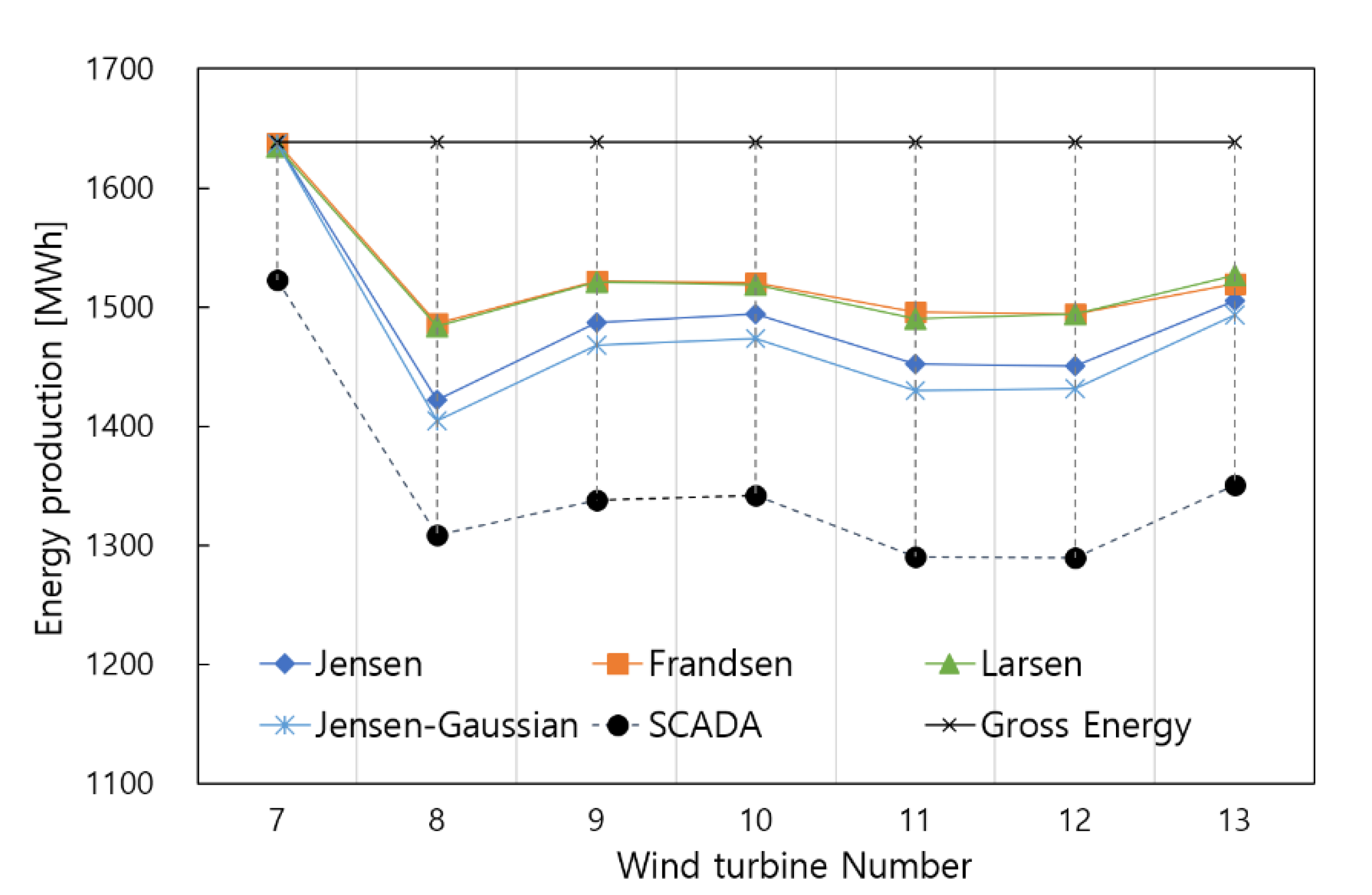
3.4. Energy Production Comparison

The differences in the energy production reflecting the wake loss in a wind farm were compared among the wake models. This expanded the comparison of power between two wind turbines to the wind farm. To remove uncertainty about the operating environment of individual wind turbines, the energy production of the Gasiri wind farm was evaluated using synchronous time operation data (WT7–WT13, seven turbines) for the undisturbed sector discussed above. The energy was calculated with the wake models using only the wind speed of the mast in the undisturbed sector and the wind direction and turbulence intensity data of the same period.

As an example, Figure 9 shows the shape of the wake and the internal wind speed deficit for each model for calculating the energy production of the Gasiri wind farm. The effect of multiple wakes was considered. The characteristics of each wake model can be observed. The Jensen and Jensen–Gaussian models show wind speed deficits due to wakes over a long distance. The Larsen model showed the largest wake diameter. As a result, the Larsen model showed that more downstream wind turbines are affected by wakes.

Figure 10 compares the energy production calculated with the wake models and the collected data for the wind turbine energy production. The four models showed differences in energy production, but the wake loss trends for each turbine were similar to the SCADA data. This indicates that, even though the wake prediction performance varied by model, the models accurately predicted the relative differences in energy loss according to the location of a wind turbine. WT7 had no wake loss because it was not affected by the wakes of other turbines in the undisturbed sector (see Figure 2 and Figure 4). The results of wake models for each wind turbine showed an average error of approximately 150 MW (approximately 10% of the SCADA energy production) compared with the SCADA data. This was due to system losses (e.g., mechanical, electrical, power curve losses, etc.) for the actual wind turbine operation. If the uncertainty about the losses is considered, the calculation results should become closer to the SCADA data. Because subjective judgment may be involved in this uncertainty, this study focused on comparing the wake models without reflecting this uncertainty. The Jensen–Gaussian model predicted the largest wake loss, and the Jensen model predicted a wake loss approximately 1% less than that of the Jensen–Gaussian model. The Frandsen and Larsen models showed similar results and predicted a wake loss approximately 3% less than that of the Jensen–Gaussian model. These differences reflected the performances of the wake models in the above comparison of the power deficit.

4. Conclusions

The power deficit due to wakes and the energy production reflecting wake loss for an onshore wind farm were compared for four analytical wake models (Jensen, Frandsen, Larsen, and Jensen–Gaussian). To apply an equivalent environment to the comparison, parameters were set according to the ambient turbulence intensity, and the turbulence intensity was determined according to the wind direction measured in the wind farm. The conclusions can be summarized as follows.

(1)

Among the analytical wake models, the Jensen–Gaussian and the Jensen model showed generally satisfactory results for the power deficit due to wakes within the scope of this study. The Frandsen and Larsen models underestimated the wake loss, but the wake diameter of the Larsen model was most similar to the actual range.

(2)

In many studies, the WDC of the conventional Jensen model was set in relation to the roughness length of the site or with the recommended values (offshore = 0.04, onshore = 0.075). This makes it difficult to ensure accuracy among sites with different environments. Peña et al.’s method of introducing a turbulence intensity that can be measured at the site appears to be appropriate within the scope of this study and can relieve the burden of determining parameters for analysts.

(3)

When the same WDC was applied in all directions, the result matched the measured values in some cases and did not in other cases. However, when the WDC was set according to the turbulence intensity measured at the site by direction, all calculation results matched well with the measured values. Therefore, the WDC should be set according to the direction when applied to analytical wake models.

(4)

The comparison of the calculated energy production of the wind farm showed that the maximum energy loss difference among the wake models was approximately 3%. The Jensen–Gaussian model predicted the largest wake loss, and the Frandsen and Larsen models predicted the smallest wake losses. However, all wake models followed the similar wake loss tendency according to the location of the wind turbine.

In summary, the Jensen–Gaussian and Jensen models are efficient analytical wake models if the environmental factors of the site are considered. In the future, further comparison and review are required in various directions with various turbulence intensities at more sites. Existing studies comparing wake models were mostly conducted in Europe or at offshore sites; this study provides an example of an onshore wind farm in Asia.

References

1. Serrano González, J.; Burgos Payán, M.; Santos, J.M.R.; González-Longatt, F. A review and recent developments in the optimal wind-turbine micro-siting problem. Renew. Sustain. Energy Rev. 2014, 30, 133–144. [Google Scholar] [CrossRef]
2. Shakoor, R.; Hassan, M.Y.; Raheem, A.; Wu, Y.K. Wake effect modeling: A review of wind farm layout optimization using Jensen’s model. Renew. Sustain. Energy Rev. 2016, 58, 1048–1059. [Google Scholar] [CrossRef]
3. Sanderse, B. Aerodynamics of Wind Turbine Wakes Literature Review; ECN: Petten, The Netherlands, 2009. [Google Scholar]
4. Lissaman, P.B.S. Energy Effectiveness of Arbitrary Arrays of Wind Turbines. J. Energy 1979, 3, 323–328. [Google Scholar] [CrossRef]
5. Jensen, N.O. A Note on Wind Generator Interaction; Risø National Laboratory: Roskilde, Denmark, 1983. [Google Scholar]
6. Katic, I.; Højstrup, J.; Jensen, N.O. A Simple Model for Cluster Efficiency. In Proceedings of the European Wind Energy Association Conference and Exhibition (EWEA), Rome, Italy, 7–9 October 1986; pp. 407–410. [Google Scholar]
7. Tian, L.; Zhu, W.; Shen, W.; Zhao, N.; Shen, Z. Development and validation of a new two-dimensional wake model for wind turbine wakes. J. Wind Eng. Ind. Aerodyn. 2015, 137, 90–99. [Google Scholar] [CrossRef] [Green Version]
8. Gao, X.; Yang, H.; Lu, L. Optimization of wind turbine layout position in a wind farm using a newly-developed two-dimensional wake model. Appl. Energy 2016, 174, 192–200. [Google Scholar] [CrossRef]
9. Sun, H.; Yang, H. Study on an innovative three-dimensional wind turbine wake model. Appl. Energy 2018, 226, 483–493. [Google Scholar] [CrossRef]
10. Xie, S.; Archer, C. Self-similarity and turbulence characteristics of wind turbine wakes via large-eddy simulation. Wind Energy 2015, 18, 1815–1838. [Google Scholar] [CrossRef]
11. Bastankhah, M.; Porté-agel, F. A new analytical model for wind-turbine wakes. Renew. Energy 2014, 70, 116–123. [Google Scholar] [CrossRef]
12. Frandsen, S.; Barthelmie, R.; Pryor, S.; Rathmann, O.; Larsen, S. Analytical Modelling of Wind Speed Deficit in Large Offshore Wind Farms. Wind Energy 2006, 9, 39–53. [Google Scholar] [CrossRef]
13. Larsen, G.C. A Simple Wake Calculation Procedure; Risø National Laboratory: Roskilde, Denmark, 1988. [Google Scholar]
14. Larsen, G.C. A Simple Stationary Semi-Analytical Wake Model; Risø National Laboratory: Roskilde, Denmark, 2009. [Google Scholar]
15. Ainslie, J.F. Calculating the flowfield in the wake of wind turbines. J. Wind Eng. Ind. Aerodyn. 1988, 27, 213–224. [Google Scholar] [CrossRef]
16. Schlez, W.; Neubert, A.; Smith, G. New developments in precision wind farm modelling. In Deutsche Windenergie Konferenz; Bremen, Germany, 2006; pp. 1–4. Available online: https://www.researchgate.net/profile/Anja_Neubert/publication/228901028_New_developments_in_precision_wind_farm_modelling/links/0c9605390a61a436b9000000/New-developments-in-precision-wind-farm-modelling.pdf (accessed on 3 February 2020).
17. Ott, S.; Berg, J.; Nielsen, M. Linearised CFD Models for Wakes; Risø National Laboratory: Roskilde, Denmark, 2011. [Google Scholar]
18. Larsen, G.C.; Madsen Aagaard, H.; Bingöl, F.; Mann, J.; Ott, S.; Sørensen, J.N.; Okulov, V.; Troldborg, N.; Nielsen, N.M.; Thomsen, K.; et al. Dynamic Wake Meandering Modeling; Risø National Laboratory Technology University: Roskilde, Denmark, 2007. [Google Scholar]
19. Larsen, G.C.; Madsen, H.A.; Torben, J.; Troldborg, N.; Troldborg, N. Wake Modeling and Simulation; Risø National Laboratory: Roskilde, Denmark, 2008. [Google Scholar]
20. Calaf, M.; Meneveau, C.; Meyers, J. Large eddy simulation study of fully developed wind-turbine array boundary layers. Phys. Fluids 2010, 22, 015110. [Google Scholar] [CrossRef] [Green Version]
21. Wu, Y.T.; Porté-Agel, F. Large-Eddy Simulation of Wind-Turbine Wakes: Evaluation of Turbine Parametrisations. Bound. Layer Meteorol. 2011, 138, 345–366. [Google Scholar] [CrossRef]
22. Cortina, G.; Sharma, V.; Calaf, M. Wind farm density and harvested power in very large wind farms: A low-order model. Phys. Rev. Fluids 2017, 2, 074601. [Google Scholar] [CrossRef]
23. Beaucage, P.; Brower, M.; Robinson, N.; Alonge, C. Overview of six commercial and research wake models for large offshore wind farms. In Proceedings of the European Wind Energy Conference Exhibition (EWEC), Copenhagen, Denmark, 16–19 April 2012; Volume 1, pp. 213–222. [Google Scholar]
24. Barthelmie, R.J.; Folkerts, L.; Larsen, G.C.; Rados, K.; Pryor, S.C.; Frandsen, S.T.; Lange, B.; Schepers, G. Comparison of wake model simulations with offshore wind turbine wake profiles measured by sodar. J. Atmos. Ocean Technol. 2006, 23, 888–901. [Google Scholar] [CrossRef]
25. Barthelmie, R.J.; Jensen, L.E. Evaluation of wind farm efficiency and wind turbine wakes at the Nysted offshore wind farm. Wind Energy 2010, 13, 573–586. [Google Scholar] [CrossRef]
26. Barthelmie, R.J.; Pryor, S.C.; Frandsen, S.T.; Hansen, K.S.; Schepers, J.G.; Rados, K.; Schlez, W.; Neubert, A.; Jensen, L.E.; Neckelmann, S. Quantifying the impact of wind turbine wakes on power output at offshore wind farms. J. Atmos. Ocean Technol. 2010, 27, 1302–1317. [Google Scholar] [CrossRef]
27. Barthelmie, R.J.; Frandsen, S.T.; Rathmann, O.; Hansen, K.S.; Politis, E.; Prospathopoulos, P.-J.; Schepers, J.G.; Rados, K.; Cabezón, D.; Schlez, W.; et al. Flow and Wakes in Large Wind Farms: Final Report for UpWind; Risø National Laboratory: Roskilde, Denmark, 2011; ISBN 9788755038783. [Google Scholar]
28. Tong, W.; Chowdhury, S.; Zhang, J.; Messac, A. Impact of different wake models on the estimation of wind farm power generation. In Proceedings of the 12th AIAA Aviation Technology, Integration, and Operations (ATIO) Conference and 14th AIAA/ISSMO Multidisciplinary Analysis and Optimization Conference, Indianapolis, Indiana, 17–19 September 2012. [Google Scholar]
29. Brusca, S.; Lanzafame, R.; Famoso, F.; Galvagno, A.; Messina, M.; Mauro, S.; Prestipino, M. On the Wind Turbine Wake Mathematical Modelling. Energy Procedia 2018, 148, 202–209. [Google Scholar] [CrossRef]
30. Göçmen, T.; Van Der Laan, P.; Réthoré, P.E.; Diaz, A.P.; Larsen, G.C.; Ott, S. Wind turbine wake models developed at the technical university of Denmark: A review. Renew. Sustain. Energy Rev. 2016, 60, 752–769. [Google Scholar]
31. Archer, C.L.; Vasel-Be-Hagh, A.; Yan, C.; Wu, S.; Pan, Y.; Brodie, J.F.; Maguire, A.E. Review and evaluation of wake loss models for wind energy applications. Appl. Energy 2018, 226, 1187–1207. [Google Scholar] [CrossRef]
32. Vermeer, L.J.; Sørensen, J.N.; Crespo, A. Wind turbine wake aerodynamics. Prog. Aerosp. Sci. 2003, 39, 467–510. [Google Scholar] [CrossRef]
33. Schepers, J.G. ENDOW: Validation and Improvement of ECN’s Wake Model; ECN: Petten, The Netherlands, 2003; p. 113. [Google Scholar]
34. Schlichting, H. Boundary-Layer Theory, 6th ed.; McGrow-Hill: New York, NY, USA, 1968. [Google Scholar]
35. Yang, K.; Kwak, G.; Cho, K.; Huh, J. Wind farm layout optimization for wake effect uniformity. Energy 2019, 183, 983–995. [Google Scholar] [CrossRef]
36. Park, J.; Law, K.H. Layout optimization for maximizing wind farm power production using sequential convex programming. Appl. Energy 2015, 151, 320–334. [Google Scholar] [CrossRef]
37. Porté-Agel, F.; Bastankhah, M.; Shamsoddin, S. Wind-Turbine and Wind-Farm Flows: A Review. Bound. Layer Meteorol. 2020, 174, 1–59. [Google Scholar] [CrossRef] [PubMed] [Green Version]
38. Crespo, A.; Hernández, J. Turbulence characteristics in wind-turbine wakes. J. Wind Eng. Ind. Aerodyn. 1996, 61, 71–85. [Google Scholar] [CrossRef]
39. Penã, A.; Réthoré, P.E.; Van Der Laan, M.P. On the application of the Jensen wake model using a turbulence-dependent wake decay coefficient: The Sexbierum case. Wind Energy 2016, 19, 763–776. [Google Scholar] [CrossRef] [Green Version]
Figure 1. Calculation of the overlap area and the wind speed deficit: (a) the intersecting area for the Jensen and Frandsen models and (b) mapping of the rotor local coordinates and wake global coordinates for the Larsen and Jensen−Gaussian models.
Energies 13 00739 g001
Figure 2. Layout of the Gasiri wind farm and turbine pairs for comparison of the power deficit.
Energies 13 00739 g002
Figure 3. Concept diagram for power deficit measurement and calculation of the wake models.
Energies 13 00739 g003
Figure 4. Turbulence intensity distribution of the Gasiri wind farm and the undisturbed sector used for analysis.
Energies 13 00739 g004
Figure 5. Comparison of wind speed deficits with the wake models (U0 = 8 m/s, TI = 0.14): (a) relative wind speed in the radial direction of the wake and (b) relative wind speed according to downstream distance.
Energies 13 00739 g005
Figure 6. Comparison of power deficits due to wakes at 3.8D: (a) U0 = 6 m/s, (b) U0 = 7 m/s, (c) U0 = 8 m/s, and (d) U0 = 9 m/s.
Energies 13 00739 g006
Figure 7. Comparison of power deficits due to wakes at 4.9D: (a) U0 = 6 m/s, (b) U0 = 7 m/s, (c) U0 = 8 m/s, and (d) U0 = 9 m/s.
Energies 13 00739 g007
Figure 8. Comparison of wind turbine power deficits according to the parameter settings of the Jensen model: (a) azimuth angle θa = (a) 30° and (b) 74°.
Energies 13 00739 g008
Figure 9. Visualization of wake models applied to the Gasiri wind farm (U0 = 8 m/s, TI = 0.14).
Energies 13 00739 g009
Figure 10. Comparison of energy production and wake loss for wake models.
Energies 13 00739 g010