Article

Aerodynamic Analysis of a Two-Bladed Vertical-Axis Wind Turbine Using a Coupled Unsteady RANS and Actuator Line Model

by
Ruiwen Zhao
1,*,
Angus C. W. Creech
1,
Alistair G. L. Borthwick
1,
Vengatesan Venugopal
1 and
Takafumi Nishino
2
1
Institute for Energy Systems, School of Engineering, The University of Edinburgh, King’s Buildings, Edinburgh EH9 3BF, UK
2
Department of Engineering Science, University of Oxford, Parks Road, Oxford OX1 3PJ, UK
*
Author to whom correspondence should be addressed.
Energies 2020, 13(4), 776; https://doi.org/10.3390/en13040776
Submission received: 4 November 2019 / Revised: 24 January 2020 / Accepted: 8 February 2020 / Published: 11 February 2020
(This article belongs to the Special Issue Recent Advances in Aerodynamics of Wind Turbines)

Abstract

:
Close-packed contra-rotating vertical-axis turbines have potential advantages in wind and hydrokinetic power generation. This paper describes the development of a numerical model of a vertical axis turbine with a torque-controlled system using an actuator line model (ALM). The developed model, coupled with the open-source OpenFOAM computational fluid dynamics (CFD) code, is used to examine the characteristics of turbulent flow behind a single two-bladed vertical-axis turbine (VAT). The flow field containing the turbine is simulated by solving the unsteady Reynolds-averaged Navier-Stokes (URANS) equations with a k - ω shear stress transport (SST) turbulence model. The numerical model is validated against experimental measurements from a two-bladed H-type wind turbine. Turbine loading is predicted, and the vorticity distribution is investigated in the vicinity of the turbine. Satisfactory overall agreement is obtained between numerical predictions and measured data on thrust coefficients. The model captures important three-dimensional flow features that contribute to wake recovery behind a vertical-axis turbine, which will be useful for future studies of close-packed rotors with a large number of blades.

1. Introduction

Climate change mitigation is vitally important for all nations in the world, given that greenhouse-gas (GHG) emissions have increased by over one-quarter since 1995 [1], as reported at the first United Nations (UN) Conference of the Parties (COP). Moreover, energy consumption by developed and developing countries has been projected to increase by 28 % from 2015 to 2040 [2]. A key approach to replacing fossil fuels as an energy source and limiting carbon release is to invest in renewable energy technology [3]. Wind and hydrokinetic energy are particularly attractive options for sustainable electricity generation from low-carbon sources [4], and are likely to become significant contributors to the electricity supply by 2030 [1]. Much ongoing research into the development of wind and tidal turbines focuses on horizontal- and vertical-axis turbines [5]. Salter [6] compared vertical-axis transverse-flow turbines with horizontal-axis axial-flow turbines in terms of flow impedance, turbulence, blockage ratio, installation, pitch change, and navigation, with tidal flow in the Pentland Firth, Scotland, in mind. Salter found that high blockage (or sweepage), vertical-axis, variable-pitch rotors could lead to substantially higher potential power generation for high impedance flows [6]. Such vertical-axis transverse-flow tidal turbines tolerate uneven seabed topography and may attain an even pressure drop by controlling the blade pitch, hence reducing wake turbulence [6]. Vertical-axis turbines thus appear to offer a promising near-term technology for tidal energy. Initial study of vertical-axis turbine (VAT) technology began in the 1970s at Sandia National Laboratories where researchers investigated vertical-axis turbine configurations, including Savonius (torque generated from drag) and Darrieus (torque generated from lift) turbines [7,8]. The Savonius turbine can accept flow from any direction and is self-starting, with low cut-in speed; however, the Savonius turbine is restricted to fewer applications due to its inefficiency at relatively low tip speed ratios [9]. Darrieus turbines have higher cut-in speed than equivalent Savonius turbines, and so rotate faster than the inflow velocity, attaining higher coefficients of performance [9,10], even though their support arms introduce additional aerodynamic drag [11]. To solve this problem, Salter and Taylor [12] proposed the innovative vertical-axis rotor system shown in Figure 1. Computational fluid dynamics (CFD) has been widely used in the systematic analyses of vertical-axis turbines [13,14,15,16,17,18,19,20,21,22,23,24,25,26,27,28,29]. Actuator-type models parameterize the turbine loading and thus reduce computational expense, but do not resolve the fine detail of the blade boundary layers [30]. Four approaches have commonly been used to represent turbines in such models, namely: actuator disc with rotation or blade element momentum (BEM) [31,32,33,34,35]; actuator disk without rotation [30,35,36]; actuator surface [37,38,39]; and actuator line [30,40,41]. BEM is an analytical method, whereas the actuator disc with rotation model is a combination of blade-element (BE) theory and CFD, which solves the Navier-Stokes equations to satisfy the momentum balance [35]. The actuator disc with rotation model is computationally efficient, but does not directly include the influence of vortices shed from blade tips on the induced velocity [31]. The uniform actuator disk without rotation model is limited in applicability because of its simplifying assumptions [37], and has proved unsatisfactory as a wake generator method for a cross-flow turbine [40]. The actuator surface technique accurately predicts the flow structure near blades and in the tip vortex region, but requires a fine mesh passing smoothly over the airfoil surface [38]. The actuator line model (ALM) [42,43] is better at capturing three-dimensional (3D) vortical structures in the near wake than actuator disc approaches [44], and so is used herein. ALM has been used to model vertical-axis turbines at low Reynolds number based on rotor diameter R e D ~ 10 4 , and of large and medium solidity (chord-to-radius ratio) at high R e D around 10 6 [30,45].
In order to simulate the wake dynamics properly, a suitable turbulence closure model is required within the CFD codes. Typically, k ε Reynolds-averaged Navier-Stokes (RANS) [46,47,48], k - ω RANS [46,48,49], and large eddy simulation (LES) [50,51] models have been used for CFD simulations of flows interacting with horizontal-axis turbines [52,53,54,55,56] and vertical-axis turbines [13,16,17,18,20,21,22,23,25,26]. Although RANS approaches are relatively inexpensive, they have the drawback that they are unable accurately to predict all types of turbulent flow [46]. LES [50,51] resolves turbulence in a partly statistical, partly explicit manner, and reduces computational cost through low-pass filtering. Even so, LES is substantially more expensive computationally than RANS, which is why it is used rather sparingly in simulations of turbulent flow past horizontal-axis turbines and vertical-axis turbines.
Typical recent applications of CFD to turbines follow. McLaren [57] reported a numerical and experimental study of the unsteady loading on a small-scale, high-solidity, H-type Darrieus turbine, based on two-dimensional (2D), unsteady Reynolds-averaged Navier-Stokes (URANS) simulations by CFD ANSYS-CFX. The study revealed the dominant effect of dynamic stall on the output power and vibration excitation of the turbine. Nobile et al. [58] later simulated 2D unsteady-flow past a Giromill wind turbine, also using ANSYS-CFX, finding that mesh resolution and choice of turbulence model had a substantial effect on accuracy, with time step having only a slight impact on the numerical results. Biadgo et al. [59] used a stream-tube approach to undertake a numerical and analytical assessment of the performance of a vertical-axis wind turbine comprising a straight-bladed fixed-pitch Darrieus turbine with a NACA   0012 blade profile using ANSYS FLUENT. These numerical predictions were compared with analytical results obtained using a double multiple streamtube (DMST) model, which exhibited inability using both CFD and DMST for the turbine to be self-starting owing to minimum and/or negative torque and performance at very low tip-speed ratios. Bachant et al. [60] developed a validated ALM of a vertical-axis turbine with both high and medium values of solidity, and tested both k ε RANS and Smagorinsky LES turbulence models in the OpenFOAM CFD framework. Bachant et al. found that RANS models running on coarse grids were able to provide good convergence behaviour in terms of the mean power coefficient. Compared with other 3D blade-resolved RANS simulations [60,61], Bachant et al.’s model achieved approximately four orders of magnitude reduction in computational expense by implementing corrections in sub-models for the effects of dynamic stall, end conditions, added mass, and flow curvature. Given that such models have focused on idealized vertical-axis turbines, further investigation into optimal practical models with fewer correction factors is still required.
Figure 1 shows a group of close-packed contra-rotating vertical-axis rotors, designed by Stephen Salter to maximise the fraction of flow passage swept [12]. Blockage is estimated to increase to 80 % given the small gaps between the rotors, which are controlled by a hydraulic ram. The rotor diameter should be at least three times the water depth in order to provide stability in pitch and roll of a single rotor, and this should be doubled for a close-packed array. This contributes to a high blockage fraction allowing generation well above the Betz limit for rotors in channels [6]. Following Buntine and Pullin [62], the design concept is based on two vortices of opposite-sign cancelling each other out, and thus conditioning the flow though the turbine while lowering the turbulence kinetic energy in the wake. The turbine downstream area will then experience less stream-wise flow variation, reducing mixing loss and therefore enhancing energy extraction. To predict the commercial feasibility of this large-scale marine hydrokinetic application, a numerical model of such devices is required.
This paper describes a numerical model of a cross-flow turbine, with the future goal of modelling close-packed tidal rotors comprising many blades. The present model is built upon a previous turbine model, which scales to thousands of cores on a supercomputer [54,56]. Although the present focus is on a single rotor, the numerical model can be applied to a large-scale turbine farm in future studies. Due to a lack of experimental data concerning this type of rotor, the numerical model is first validated against experimental measurements from a two-bladed H-type wind turbine, and then used to predict turbine loading and investigate vorticity distribution in the vicinity of the rotor.
A newly developed, efficient, parallelised, numerical model of vertical-axis turbines, with a fixed tip-speed ratio system and with a torque-controlled system, is presented in the following sections. This computationally efficient numerical model is coupled with and is developed within the OpenFOAM CFD framework. Unique features of the present model include torque control and active pitch mechanisms. For brevity, only the torque-controlled system is presented in this paper; pitch control mechanisms for solving the dynamic stall problem as well as performance optimization [63,64] will be explored in future work. We believe that the application of the present model to a torque-controlled vertical-axis turbine gives new insight into the aerodynamic behaviour of vertical-axis wind turbines, in particular the difference in behaviour between an idealised turbine with fixed tip-speed ratio and a more practical turbine with torque control.

2. Mathematical Model

Flow past a single vertical-axis turbine (VAT) with an arbitrary number of blades is simulated using an adapted version of the Wind and Tidal Turbine Embedded Simulator (WATTES), which is an efficient, parallelised, two-way coupled turbine model of horizontal-axis turbines, scaling to thousands of computing cores [54,56]. We denote the newly developed model WATTES-V. A preparatory set-up of the original WATTES model using the OpenFOAM CFD solver was conducted to ensure the codes were correctly coupled [65]; details of the software architecture are provided in Appendix A. This prerequisite ensures that WATTES-V model benefits from the advantages of the original model. One unique feature of the modified WATTES-V model is that it enables torque control; the main benefit of torque-controlled models is their prediction of the dynamic response of the turbine to the flow [52,53,54]. The mathematical formulation of WATTES-V is provided below.

2.1. Frame of Reference

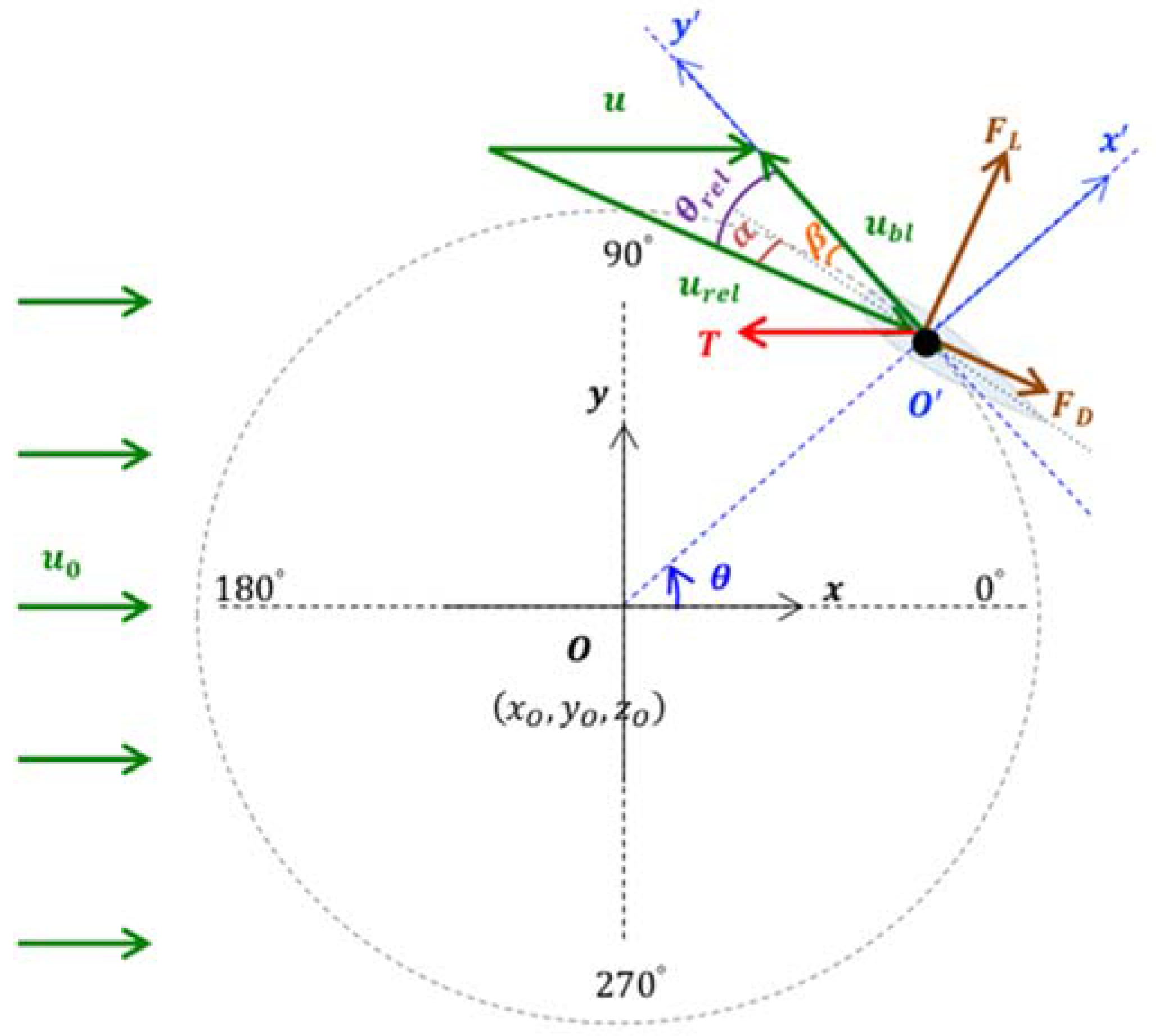
To calculate the body forces, the coordinates of nodes in the mesh are first translated to the frame of reference of the rotor, in a similar manner to the original WATTES model [54]. The centre of the vertical-axis turbine is located at position O (see Figure 2), where x O = ( x O , y O , z O ) . The azimuthal angle, which describes the orbital path taken by the first turbine blade, is denoted θ . In WATTES-V, θ starts from the x -axis, as indicated in Figure 2. The coordinates of a blade reference frame are denoted x , y , z , with O ( x ,   y ,   z ) the origin of the new reference system. In the blade reference frame, the coordinates of a transformed point at position x = ( x ,   y ,   z ) are:
x = ( x ,   y ,   z ) = R ( θ ) [ x x O y y O z z O ] ,
where
R ( θ ) = [ cos θ sin θ 0 sin θ cos θ 0 0 0 1 ] .
Similarly, the localised velocity at a given point is u = ( u ,   v ,   w ) , and this is transformed to the rotor’s frame of reference as u = R ( θ ) u . Once in this frame of reference, the model calculates the momentum source terms, and then a second transformation takes place before passing these back to the CFD solver (cf. Creech et al. [54]). To simplify the notation, we denote the transformed coordinates and velocity as x and u hereafter.

2.2. Lift and Drag Calculations

The actuator line method (ALM) [43] creates a distribution of body forces along a set of line segments representing the blades of a turbine. For each turbine rotor, only grid points found within the hollow cylindrical volume V traced out by the rotating blades are considered.
The lift and drag force vectors per unit span on a blade are given by:
f L = l i f t u n i t   s p a n = 1 2   ρ   C L ( α , R e )   | u r e l | 2   c ( z )   e L ,
f D = d r a g u n i t   s p a n = 1 2   ρ   C D ( α , R e )   | u r e l | 2   c ( z )   e D ,
where ρ is the fluid density, and C L and C D are the lift and drag coefficients, which depend on the angle of attack α and the Reynolds number R e of the flow over the blade. The magnitude of relative velocity of the fluid over the blade is | u r e l | , and c ( z ) is the blade chord length, which can vary along the blade span, but in the present case is constant. As the blades are parallel to z-axis, this is a function of z . The unit vectors e L and e D are in the direction of lift and drag respectively. Values of C L and C D are given in tabulated form [54], and as with most models, these are derived from an assumption of two-dimensional flow over the blade. Figure 2 shows a schematic diagram illustrating a turbine blade with chord, pitch, and path of a single blade. The diagram also indicates the force component vectors that provide loading on the blade. The black dashed circle represents the circular trajectory of a blade.
The relative velocity u r e l is calculated for each point within the control volume V at a radial distance r from the rotor center (along z -axis) as
u r e l = u u b l ,
where u b l is the blade velocity. For a vertical-axis turbine, the magnitude of u r e l is
u r e l = | u r e l | = u 2 + v 2 + u b l 2 + 2   u a z   u b l ,
where u b l = r ω b l , and ω b l is the angular velocity of blade. Note that the spanwise velocity component is neglected here, because the spanwise component of flow velocity is assumed to have minimal impact on the performance of the blade, and so tip-loss effects can be ignored. The azimuthal component of the fluid velocity is given as
  u a z = 1 r   ( x   v y   u ) .
This is necessary to account for the rotation of the flow, as lift and drag forces act to turn the blades and the generator, resulting in an equal and opposite reaction force acting on the flow, causing it to rotate in the opposite direction to that of the blades [54].
The flow angle relative to that of the fluid is
θ r e l = tan 1 ( u   cos θ + v   sin θ   u   sin θ + v   cos θ ω b l r ) .
The local angle of attack is then computed from θ r e l as follows:
α = θ r e l β ,
where the local blade angle β is given by
β = β p + β t .
The blade pitch angle β p can be actively controlled, as with [54], but for the present validation work it is kept constant at β p = 0 . The local blade twist angle β t is calculated from the blade geometry but we consider straight blades and hence β t = 0 in the present test cases.
Lift and drag forces per unit span are then calculated using the WATTES-V actuator line representation of each blade, which utilises a two-dimensional Gaussian regularization kernel η i ( d i ) [56]:
F L = i = 1 N b l η i ( d i ) f L i , F D = i = 1 N b l η i ( d i ) f D i ,
where N b l is the number of blades, d i is the shortest distance between a given point and the i th actuator line. The pointwise lift and drag per unit span, f L i and f D i , are obtained from Equations (3) and (4). A two-dimensional Gaussian regularization kernel operates in the blade azimuthal direction and smears the solution in a circle [56], such that:
η i ( d i ) = 1 2 π σ 2 e d i 2 2 σ 2 ,
where the distance from the i th vertical actuator line is d i = ( x x i ) 2 + ( y y i ) 2 , with x i and y i the local coordinates of blade i , x and y are the point coordinates, and the standard deviation σ determines the width of the Gaussian kernel.
The value of σ was chosen carefully so that it is neither too large (smeared solution) nor too small (extremely high resolution, and correspondingly small time step) [56]. Experiments determined that numerical stability was optimal when the Gaussian width was set to twice the local cell length, Δ x , as also by Troldborg [30,43]. Other researchers have investigated the effect of the standard deviation (or projection width) on accuracy and stability: Schito and Zasso [30,66] found that the equivalent of the mesh cell width was ideal; Jha et al. [30,67] recommended using an equivalent elliptic planform for its calculation; Martinez-Tossas and Meneveau [30,68] used two-dimensional potential flow analysis to determine the optimal projection width; Tennekes and Lumley [69] recommended the projection width to be of the order of the momentum thickness θ m t [30]. Here, the Gaussian width related to mesh size is estimated as Δ x V c e l l 3 where V c e l l is the cell volume. Following Bachant et al. [30], an additional factor C m e s h = 2.0 is introduced, and non-unity aspect ratio cells incorporated using σ = 2 C m e s h Δ x . This meant that 95.45 % ( d i 2 σ ) of the Gaussian distribution was captured within the numerical simulation. It should be noted that σ is a tuning factor that should be adjusted to the particular circumstances under consideration.
The tangential F t and normal F n components of body forces acting on the fluid, which are in the opposite directions to the force acting on the blade, are given by
F t = F L sin θ r e l F D cos θ r e l , F n = F L cos θ r e l + F D sin θ r e l .
Body force components acting on the fluid in x and y -axis directions are
F x = F t sin θ + F n cos θ , F y = F t cos θ + F n sin θ ,
where F x is also the net thrust component of the fluid to the turbine. Note that F z = 0 , as three-dimensional flow effects on performance are neglected.
All the calculated force terms are then transformed into body force components, and passed back to OpenFOAM as momentum sources in the Navier-Stokes momentum equation for an incompressible Newtonian fluid given by:
D u D t = 1 ρ   p + ν 2 u + 1 ρ F ,
in which u is velocity field vector, ρ is fluid density, p is pressure, ν is the kinematic viscosity, t is time, and F is the body force vector exerted on the fluid.

2.3. Power and Torque Calculation

The lift and drag force components acting on the blade exert an equal and opposite reaction on the flow [54]. This occurs at each point within the control volume V , which is a hollow cylinder of thickness 4 σ with a radius equal to that of the rotor. This is used to calculate the instantaneous power output of the turbine at time t . L is blade length and d l is span-wise blade element dimension. The total torque acting on the fluid within the hollow cylindrical volume V is
τ f l = V r × F   d V .
The torque on the fluid acts in the opposite direction to the torque that turns the generator to create power τ p o w and the torque due to the moment of inertia of the blades τ b l , such that τ f l = ( τ p o w + τ b l ) . Here we have dropped the vector notation for torque, given that the torque vectors are all parallel to the z -axis. For a fixed-speed turbine,
τ p o w = τ f l .
Using the generator efficiency model from [56] to calculate power, we have
P r e a l = E d E g P i d e a l ,
where P r e a l is the actual power, E d is the drive train efficiency, E g is the generator and power conversion efficiency, and P i d e a l is the instantaneous power output of the turbine.

2.4. Torque Control and Thrust

As with the original WATTES, the moment of inertia of the rotor must be defined with torque to accelerate the blades in WATTES-V. Here, it is assumed the majority of each blade’s mass is at distance R , the rotor radius, from the centre of the rotor, and that each blade is identical to the other. The moment of inertia for a vertical-axis turbine can then be written as
I = N b l   m   L   R 2 ,
where N b l is the number of blades, m is the mass per unit span, and L is the span length of each blade. We can then use I to define τ b l , the torque that accelerates the blades. More details of this, and the time integration scheme used, can be found in [54].
The instantaneous thrust is calculated by integrating the x -direction body forces over the turbine control volume, that is
T = V F x d V .

3. Turbine Parameterization

Due to the lack of an experimental prototype, the present vertical-axis turbine model is validated against data from wind tunnel experiments involving a two-bladed H-type vertical-axis wind turbine (VAWT) that was equipped with sensors to measure thrust and side loading on the turbine [70]. The experimental data were collected at the Open Jet Facility at Delft University of Technology [70], which comprised a closed loop open jet air flow of 2.85   m   ×   2.85   m outlet cross section. The wind tunnel test section was 13   m long. Table 1 lists the turbine model parameters, derived from [70].
The numerical model neglects the rotor shaft and support struts, and utilizes an unsteady Reynolds-averaged Navier-Stokes (URANS) formulation with k - ω shear stress transport (SST) turbulence closure scheme in OpenFOAM. The URANS approach is an attractive, computationally inexpensive prospect for far-wake simulation [55]. The k - ω SST turbulence model used is the original Menter model [71], which has been used successfully for many different types of flows. The SST (shear stress transport) turbulence model combines the k - ε model in the free shear flow, with the k - ω model in the near wall boundary regions. It is a robust two-equation eddy-viscosity turbulence model [71]. We would like further to develop our vertical-axis turbine model by adding solid support struts as a conventional turbine, which would enable our model to be used to represent a wide range of vertical-axis turbines and turbine farms in the future. We thus chose to use a k - ω SST model instead of a k - ε model in this paper. Whilst there would be undoubted merit in exploring the effect of different turbulence models on the results, as undertaken by Barthelmie et al. [72], this is beyond the scope of the present work, but is recommended for future study.
The goal of the validation test is to check the ability of the newly developed numerical model WATTES-V to determine the thrust and side loading on the turbine for different values of azimuthal angle and tip speed ratio, with future applications to multi-bladed vertical-axis turbines in mind. This also enabled us to investigate the difference in behaviour between an idealised turbine with fixed tip-speed ratio and a more realistic turbine with torque control.

4. Results and Discussion

The three-dimensional (3D) computational domain is configured to be similar to the physical test-section containing the model-scale wind turbine [70]. The domain cross-sectional dimensions are 2.85   m   ×   2.85   m , which match the outlet size of the flow contraction section located upstream of the open test section used in the experiments. However, given that the open test section allowed the flow to expand in the Open Jet Facility, it should be noted that the present computational domain (with straight side-walls not allowing the flow to expand) is likely to cause a blockage effect stronger than that in the experiments. The turbine is located 4.5   m downstream of the inlet, at mid elevation of the tunnel. Figure 3 shows a mesh slice in the x - y plane, generated using blockMesh and snappyHexMesh utilities in OpenFOAM. The mesh is refined by a factor of 2 using a hexahedral mesh in a rectangular region containing the turbine and near-wake field, following [73]. Here, mesh refinement is controlled by the number of cells in the ( n x , n y , n z ) directions. Simulations were performed using the pimpleFoam solver, a merged PISO-SIMPLE algorithm. It should be noted that the azimuthal angle θ used in [70] starts from the y -axis, as indicated in the second figure in [70]. In accordance with measurements from [70], the azimuth θ described in the following sections has been transformed to the experimental coordinate system.
Initial and boundary conditions are selected to be approximate those in the physical wind tunnel test section. The inflow velocity is fixed at 4.01   m / s inflow. Lateral, bottom, and top walls of the computational domain are represented numerically by slip-flow conditions. A zero pressure gradient is applied at the inlet, and a fixed pressure prescribed at the outlet with zero gradients for other flow variables. Inlet turbulence intensity is ~ 10 % , with turbulence kinetic energy k of 0.24   m 2 / s 2 and specific dissipation rate ω of 1.78   s 1 . It should be noted that the computational time for a simulation of ten revolutions was about six core hours for a parallel computation using four computing cores.

4.1. Validation and Grid Sensitivity Studies

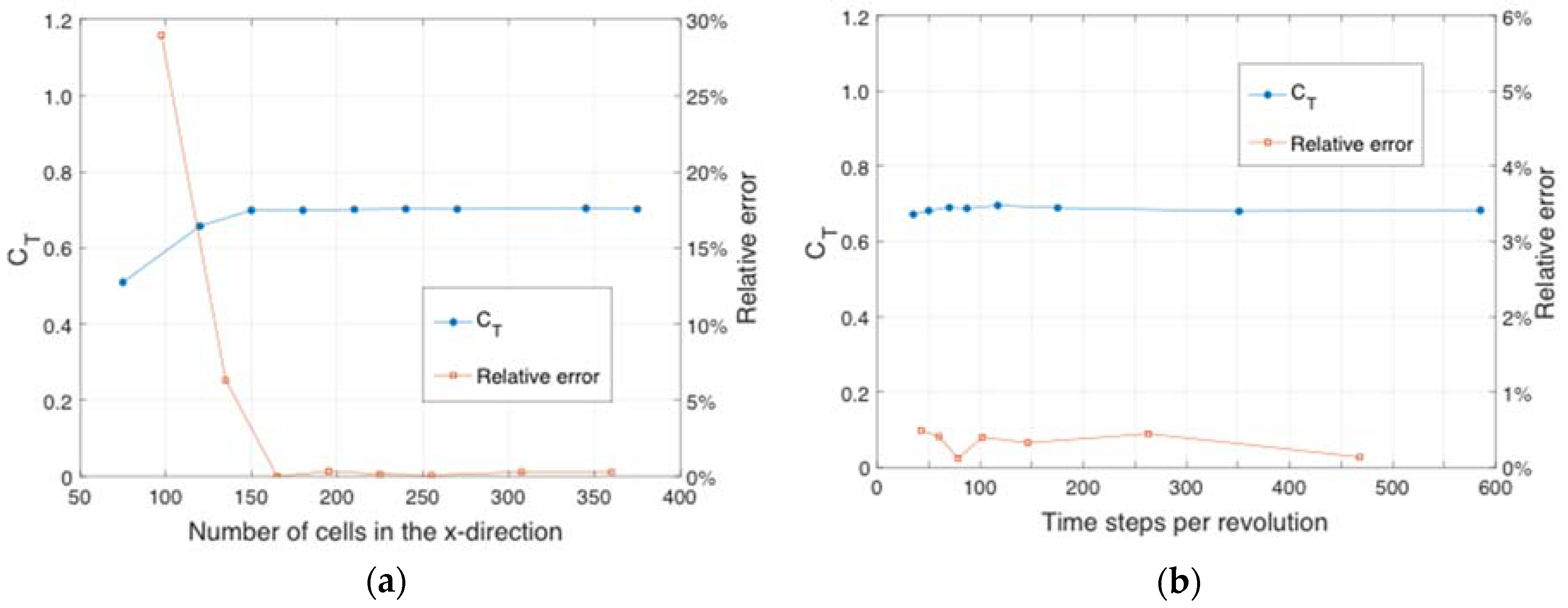
Sensitivity studies concerning spatial and temporal resolution will be discussed in this section. We first considered the convergence of turbine mean thrust coefficient for a tip-speed ratio of 3.3 , shown in Figure 4. Mesh refinement is conducted by changing the number of cells in the x -direction with a fixed cell aspect ratio and mesh topology. The relative error [74] between the results from the two finest meshes is below 0.5 % , indicating that mesh convergence had been achieved. The spatial mesh resolution is hitherto set to 150 cells in the stream-wise x -direction, with about 18 covering a single blade chord, (where the error between the finest mesh and the mesh employed is about 0.4 % ), giving a total number of 6.72 × 10 5 cells in the 3D simulation. Details of a mesh sensitivity study of the near-wake vorticity field are provided in the first part of Appendix B. Figure 4b displays time-step resolution test data, evaluated on the 3D grid with 150 cells in the x -direction. The relative error is below 0.5 % , indicating low sensitivity to temporal resolution. In all these convergence tests, the Courant–Friedrichs–Lewy (CFL) number [75] is below 0.58 . In this study, we employed Δ t = 0.03   s , corresponding to 120 time steps per revolution, giving a CFL number of 0.23 . Simulations were carried out lasting at least 10 revolutions, with periodic convergence reached after 9 revolutions when the difference in maximum turbine thrust between successive revolutions was 0.06 % .

4.2. Two-Bladed H-Type Vertical-Axis Wind Turbine: Fixed Tip Speed Ratio

We now present results obtained for a two-bladed H-type vertical axis wind turbine where the tip speed ratio is set to a fixed value. Figure 5 compares the numerical predictions and measured thrust and lateral force components on the rotor for an incoming flow speed of 4.01   m / s , a fixed pitch angle of 0 ° , and a tip-speed ratio (TSR) of 3.7 . The measurements were averaged over 22 turbine rotations. It can be seen that the numerical predictions and experimental measurements of the force components in both x - and y - directions are similar in terms of amplitude and profile, with the maximum thrust loading experienced at the blade azimuth at 90 ° and 270 ° .
We next study the effect of tip speed ratio on the mean thrust coefficient, carrying out numerical simulations that reproduce the experimental tip speed ratios of 2.7 , 2.9 , 3.1 , 3.3 , and 3.7 . There is good overall agreement in the general trends of the model predictions and experimental data on the x -direction force coefficient as a function of TSR (Figure 6). The obvious overshoot is most likely caused by the blockage effect. The actual cross section of the experiments is supposed to be much wider than the outlet width of the open jet, where the blockage effect in the numerical simulations is stronger than in the experiments. A lack of information on the turbulence intensity of the wind tunnel experiments may also be a factor behind the discrepancy. Appendix B provides a more detailed discussion of the sensitivity of the model to inlet turbulence level and downstream domain length. It is found that the results are sensitive to inlet turbulence intensity, but not to a doubling of downstream domain length.
Figure 7 depicts the variation in force coefficients in the x - and y - directions with azimuthal angle for three selected TSR values. Amplitudes of both the predicted and measured force coefficients increase progressively with TSR. This is because the blade velocity and hence the relative flow velocity experienced by the blades increase as TSR is raised; the increased velocities then augment the blade load. There appears to be satisfactory overall agreement between the numerical predictions and measurements of C T and F y for TSR values of 3.3 and 3.7 . However, there are more noticeable discrepancies between the predicted and measured values of C T and F y for TSR 2.9 ; this is because the angle of attack exceeds the critical angle for parts of each rotation when TSR is 2.9 , causing stall to occur.
Figure 8 illustrates the reduction in the lift coefficient that occurs at TSR = 2.9 as the critical angle of attack of the foil is exceeded at such a low value of TSR. It should be noted that data for cases where TSR < 2.5 were excluded from the experimental analysis because of this kind of poor aerodynamic performance [70]. The higher TSR values (i.e., > 2.9 ) considered in the validation case are sufficiently large to be outside the range in which dynamic stall is likely to occur, and the predicted and measured values of C T and F y almost match. However, as the local velocity of the blades increases, so does the local Reynolds number based upon chord length, R e c , which in turn affects the dynamic performance of the airfoil. In future work, the dynamic stall problem could be solved for the modelled vertical-axis turbines by controlling the blade pitch to attain an even or higher pressure drop along the whole diameter of a rotor. As shown in Figure 8, the angle of attack on each blade does not exceed 20 ° at TSR = 2.9 (and higher), and so the dynamic stall problem is not encountered here.
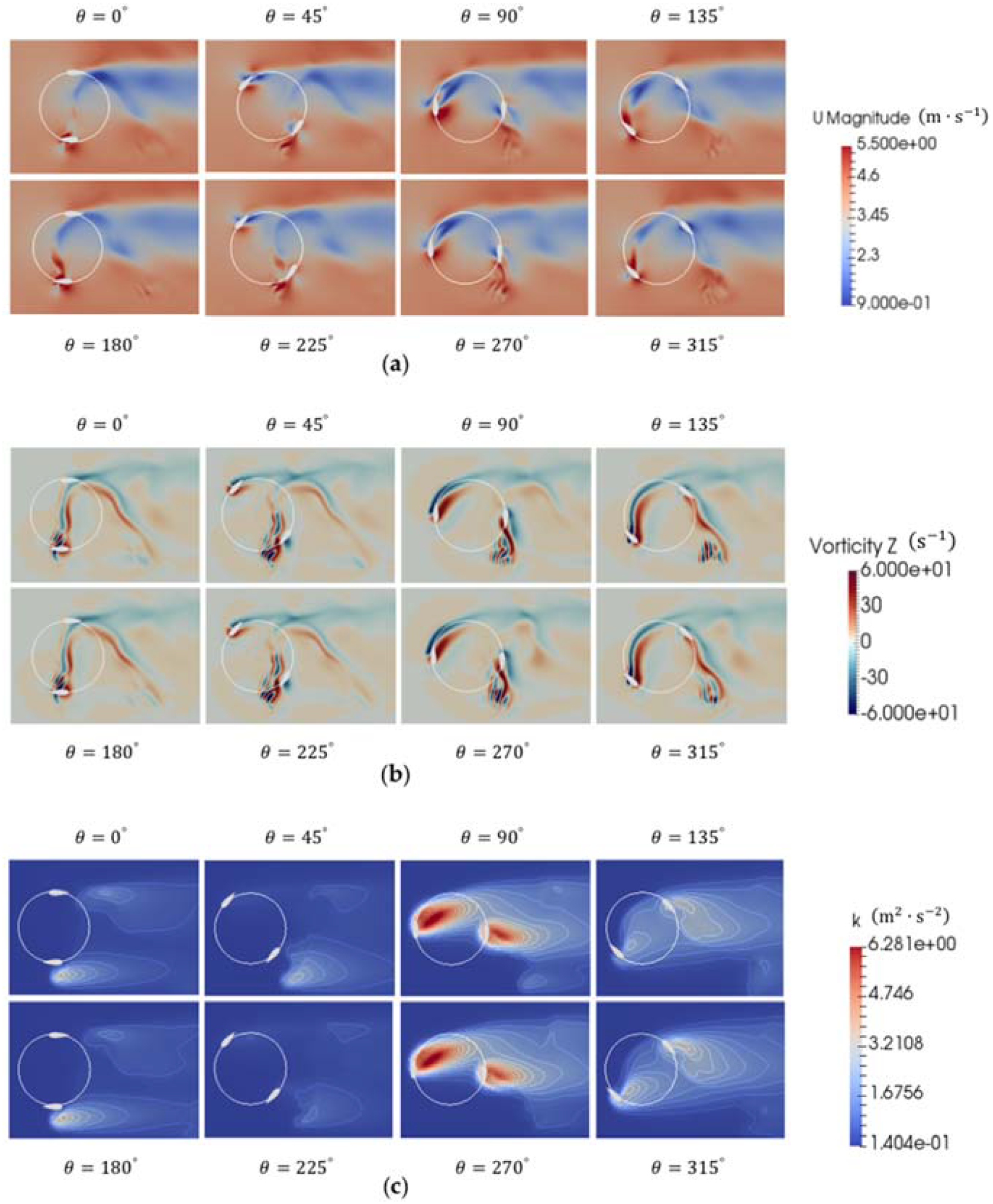
Figure 9 shows plan views of the evolving velocity magnitude, vorticity z -component fields, and turbulence kinetic energy contours in the horizontal x y plane at eight different phases during one revolution of the 2-bladed VAT operating at TSR = 3.7 . The white blades are shown for interpretation only, and the k - ω SST model behaves like a k - ε model even near the blades (as in the free shear flow). θ is the azimuthal angle of the first blade measured from the experimental turbine in the anti-clockwise direction. The incoming flow passes through an annulus mapped out by the anti-clockwise rotating turbine, with vorticity generated on the surface of the blade and a turbulent wake developing downstream. The rotor interacts with its own wake, especially for azimuthal angles of 90 ° and 270 ° , causing the thrust to increase. Vortex shedding starts to occur when the first rotor blade reaches an azimuthal position of about 180 ° . Vortices detach periodically from the turbine, and move to the downstream low-pressure wake field. This vortex shedding process drives oscillations in the local flow field affecting the forces on the rotor blades. The highest turbulence kinetic energy is observed at about 90 ° or 270 ° of the azimuthal position.
Figure 10 illustrates an instantaneous three-dimensional vorticity field around the turbine. It can be seen that a smooth, quasi-two-dimensional shear layer, as a consequence of using URANS turbulence modelling, is created behind a blade moving towards the upstream direction. The blade then turns into the downstream direction and sheds large and more three-dimensional (spanwise-modulated) vortices. Strong tip vortices then interact with the shed vortices, and create a complex downstream wake field.
Figure 11 shows the variance in angle of attack experienced by the two blades during a single revolution. This arises due to the blade shedding sheet vortices, which then break up into three-dimensional turbulence when the blade moves towards the downstream direction, giving greater variation in the angle of attack across the blade. This highlights where the flow around the blades experiences strong variations, and this coincides with where vortex detachment occurs during each revolution.
The variance is calculated from:
Var ( X ) = E [ X 2 ] E [ X ] 2 = i = 1 N n d ( p i   x i 2 ) μ 2 ,
where X is a discrete random variable, E is an expectation operator, N n d is the total number of nodes in the region of the blade, p i is the probability mass function, α i is the local angle of attack at point i , and μ = E [ X ] (or α ) is the mean weighted value of angle of attack, given by
p i   x i 2 = p i   α 2 = η i ( d i )   α i 2 η ( d i ) = η i ( d i )   α i 2 i = 1 N n d η i ( d i ) ,
and
μ = i = 1 N n d η i ( d i )   α i η ( d i ) = i = 1 N n d η i ( d i )   α i i = 1 N n d η i ( d i ) .
A similar method was used in an earlier study [56]. The maximum variance occurs at the first rotor blade azimuth of 180 ° and the second blade azimuth of 0 ° or 360 ° (Figure 11). This three-dimensionality might be due to shear flow instability, which is similar to that observed for a 2D pitching airfoil when its angle of attack decreases. The variance profiles are asymmetric with azimuthal angle, with large changes occurring after vortex detachment.
Figure 12 presents an overview of the downstream wake evolution behind the turbine with the distribution of the mean stream-wise velocity and the turbulence kinetic energy in the near-wake region at x / D = 1 . The mean velocity field for TSR = 3.7 , shown in Figure 12a, is obviously asymmetric in the transverse ( y ) direction. The mean wake deficit in Figure 12c describes the characteristic of the mean velocity as it recovers rapidly on the coarse mesh [77,78,79] for the three selected tip speed ratios. Minimum values of mean velocities were found predominantly to occur at y   ~   0.35 D . In the bypass flow at y / R > 1.5 , the stream-wise velocity component reaches approximately | U / U 0 | = 1.1 , due to the blockage effect. Turbulence kinetic energy profiles in the vicinity of the rotor also exhibit clear asymmetry, with a peak at y / R ~ 0.2 .
Figure 13 shows the lateral profiles of stream-wise mean velocity (Figure 13a–c) and turbulence kinetic energy (Figure 13d–f) at x = 1 D 5 D downstream for TSR = 2.9 , 3.3 , and 3.7 respectively. The near-wake region (roughly x / D < 2 ) is characterised by a low-momentum area isolated from the ambient flow in the presence of vortices, whereas the transition region (roughly 2 < x / D < 5 ) is characterised by fast momentum recovery, high levels of turbulence, and expansion of the wake [80]. In Figure 13a–c, the asymmetry of mean velocity profiles is more visible closer to the turbine centre in the near-wake region. In Figure 13d–f, the mean turbulence kinetic energy profiles are W-shaped. The two peaks are in accordance with those of the mean velocity profiles; however, the maximum peak of the turbulence kinetic energy is located on the side with negative y , not on the side with positive y where the largest velocity deficit is observed. This is presumably due to the (aforementioned) large vortices that shed when the blade motion is in the same direction as the flow velocity in this area. These vortices play a key role, and affect mixing between the ambient flow and the low-velocity wake flow. Comparing the shape of these wake deficits with results from other published models of vertical-axis turbines [30,80], it can be stated that these characteristics of the mean velocity and turbulence kinetic energy profiles agree qualitatively with these previous studies of vertical-axis turbine wakes. For example, the shape of the mean stream-wise velocity profile of the present model corresponds well with those of experimental profiles presented in Figure 9 (left) in [30] and Figure 5. (a) in [80], where the lowest values of U / U 0 are both located close to y = 0.35 D . The shape of the turbulence kinetic energy profile exhibits good agreement with the experimental profile in Figure 9 (right) in [30], especially for areas in the vicinity of both peaks, and is in even better accordance than the University of New Hampshire reference vertical-axis turbine (UNH-RVAT) model used in [30]. For the Edinburgh turbine (see Figure 1), the bending stresses at both ends are decreased by a factor of nearly four, with the red rings suppressing tip-vortex losses caused by the adjacent foils at different angles. Although the rings experience drag, the spoked wheel could well be a more efficient load-bearing structure than a tower, which experiences vortex shedding in addition to drag [65].

4.3. Two-Bladed H-Type Vertical-Axis Wind Turbine: Torque-Controlled Tip Speed Ratio

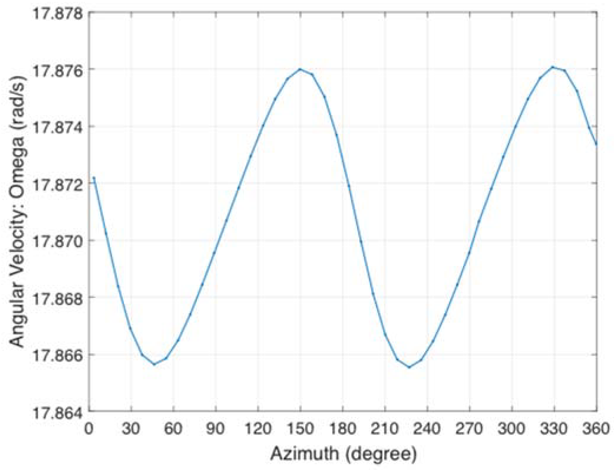
We now present results obtained for a two-bladed H-type vertical axis wind turbine where the rotational speed of the blades is controlled by the torque. Figure 14 shows the limit cycle variation of the turbine angular velocity against azimuthal angle of the first blade, where the rotor is dynamically driven by the incoming wind flow. The predicted mean angular velocity ω in the torque-controlled model is 17.87   r a d / s . This value is slightly smaller than that of the initial angular velocity (of 17.88   r a d / s , calculated from ω i n i = TSR · u 0   R ) used to set the rotor in motion. In general, the turbine settles down until the energy losses due to drag and the generator are balanced by the energy extracted from the fluid through lift.
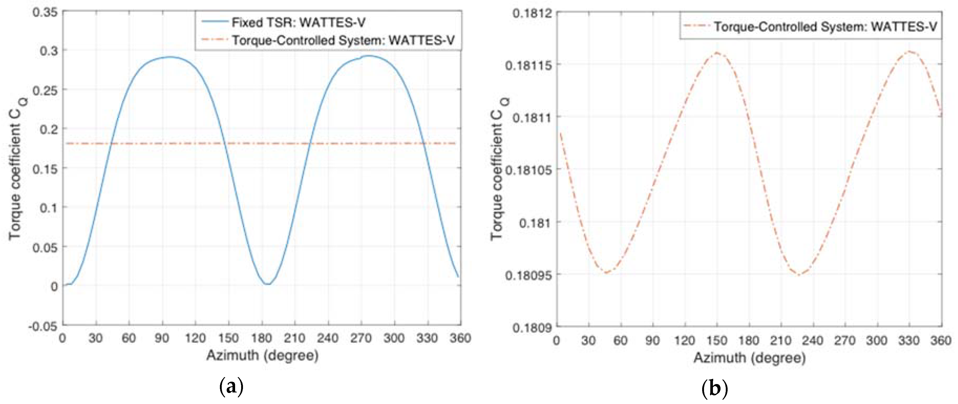
The torque coefficient C Q is calculated by using the dynamic generator torque data as C Q = τ p o w 1 2   ρ   u 0 2   ( D   L )   R . Figure 15 shows a comparison of the torque coefficient results obtained for the fixed tip-speed ratio and torque-controlled cases. As shown in Figure 15a, the predicted C Q for the model with fixed tip-speed ratio keeps changing through one rotor-revolution, whereas the C Q for the torque-controlled model remains almost constant with azimuthal angle. Figure 15b presents an enlarged graph of C Q variation for the torque-controlled case, where C Q experiences less than 0.1 % change with azimuthal angle. This can be explained by the high mass density of the blades, whose angular momentum becomes a source of torque for the generator when fluid torque drops. This behaviour is not present in the fixed tip-speed model, as the torque accelerating the blades is by necessity always zero.
Figure 16 displays the thrust and lateral force coefficients as functions of the azimuthal angle obtained from the fixed tip-speed ratio model, the measured data [70], and the torque-controlled model (where the thrust derives purely from the aerodynamic flow driving the turbine). Satisfactory overall agreement can be seen between the numerical predictions and measurements of C T and F y for TSR values of 3.3 , as shown in Figure 16a,b. However, there are still some noticeable discrepancies evident between the torque-controlled model predictions, the fixed tip-speed ratio model predictions, and the experimental measurements, especially regarding F y in Figure 16b.

5. Conclusions

This paper has presented a newly developed, efficient, parallelised, numerical model that simulates turbulent flow through vertical-axis turbines with a torque-controlled system, as well as with a fixed tip-speed ratio system. This computationally efficient numerical model WATTES-V of a single cross-flow turbine was developed within the OpenFOAM CFD framework. The model is based on actuator line theory, and combines classical blade element theory, an unsteady Reynolds-averaged Navier–Stokes flow model, and a k - ω SST turbulence model.
This numerical model with fixed tip-speed ratio was validated against experimental data acquired from an H-type 2-bladed vertical-axis wind turbine [70]. The model gives numerical predictions in satisfactory overall agreement with experimental data on thrust and lateral loading. It is planned that the present cross-flow turbine model will be employed in future research on wakes behind close-packed contra-rotating vertical-axis tidal turbines [12]; hence, the support struts and tower shaft for a normal H-type vertical-axis turbine have not been considered herein. The present results show that vortex shedding occurs at the azimuthal position of the first rotor blade, at about 180 ° . Vortices detach periodically from the turbine, and the resulting interactions create a complex downstream wake. The angle of attack for each blade did not exceed 20 ° in the present study, and so dynamic stall could be ignored. However, for future studies based on the present numerical model, either a dynamic stall model could be added as a correction, or a pitch-controlled system could be used to limit the angle of attack to an optimum value.
The wake field predicted by the present vertical-axis turbine model with fixed tip-speed ratio may be divided into two distinct regions. The near-wake region features a low-momentum zone where vortices shed from the turbine have a significant influence on the low-velocity region. The wake deficit in the transitional-wake region exhibits momentum recovery due to entrainment of ambient flow into the wake, and generates asymmetric velocity profiles about the wake centreline. Analysis of wake turbulence behind a single vertical-axis turbine could facilitate better understanding of key flow features that contribute to wake recovery behind an array of close-packed contra-rotating vertical-axis turbines in future work. The sensitivity study on the turbulence parameters of the inlet flow and the downstream domain length (discussed in the Appendix B) should be useful for future experimental tests and numerical validations.
Dynamic predictions made by the present numerical model with torque-controlled tip-speed ratio are in satisfactory overall agreement with corresponding results from the fixed tip-speed ratio model and experimental data [70] on thrust and lateral loading. In the former case, the rotor is demonstrably driven by the blade-generated lift, which is counteracted by the torque that accelerates the blades and turns the generator. The present model should be useful in the future by enabling predictions of the dynamic response of practical vertical-axis turbines to unsteady flow.

Author Contributions

Funding acquisition, V.V.; Investigation, R.Z.; Methodology, R.Z. and A.C.W.C.; Supervision, A.C.W.C., A.G.L.B., T.N. and V.V.; Writing—original draft, R.Z.; Writing—review & editing, A.C.W.C., A.G.L.B. and T.N. All authors have read and agreed to the published version of the manuscript.

Funding

This research was funded by Flowturb project.

Acknowledgments

The first-named author is supported by funding awarded by the China Scholarship Council and the University of Edinburgh. The authors thank Stephen Salter for insightful suggestions that have informed the present research. The work was partly funded by the UK Engineering and Phyiscal Sciences through the FloWTurb project (EP/N021487/1).

Conflicts of Interest

The authors declare no conflict of interest.

Nomenclature

VariableDescription
c Blade chord ( m )
C L , C D Lift and drag coefficients
d i Smallest distance between a given point and the i th actuator line ( m )
e L , e D Unit vectors in lift and drag directions
E d , E g Drive train efficiency, conversion efficiency
f L , f L i Lift component per unit span on the i th blade ( N / m )
f D , f D i Drag component per unit span on the i th blade ( N / m )
F L , F D Turbine lift and drag forces per unit span ( N / m )
F t , F n Tangential and normal forces per unit span ( N / m )
F x , F y Body forces per unit span in x - and y-axis directions ( N / m )
I Moment of inertia ( kg · m 2 )
L Blade length ( m )
m Blade mass per unit span ( kg / m )
N b l Number of blades
P r e a l , P i d e a l Actual power, instantaneous power ( W )
r Radial distance from the rotor centre ( m )
R e Reynolds number
T Thrust ( N )
u Local inflow velocity ( m / s )
u 0 Freestream velocity ( m / s )
u b l Blade velocity ( m / s )
u r e l Flow relative velocity (m/s)
u a z Azimuthal component of the fluid velocity ( m / s )
u ,   v ,   w Three components of local velocity ( m / s )
( x ,   y ,   z ) Coordinates in the original reference frame ( m )
( x ,   y ,   z ) Coordinates in the blade reference frame ( m )
α Angle of attack ( rad )
β Corrected pitch ( rad )
β p Blade pitch ( rad )
β t Local blade twist angle ( rad )
η i Gaussian regularization
θ Azimuthal angle ( rad )
θ r e l Relative angle ( rad )
ρ Fluid density ( kg / m 3 )
σ Width of the Gaussian kernel
τ f l , τ p o w , τ b l Fluid torque, generator torque, blade torque ( N · m )
ω b l Blade angular velocity ( rad / s )
ω ˙ Blade angular acceleration ( rad / s 2 )

Appendix A

Model Architecture

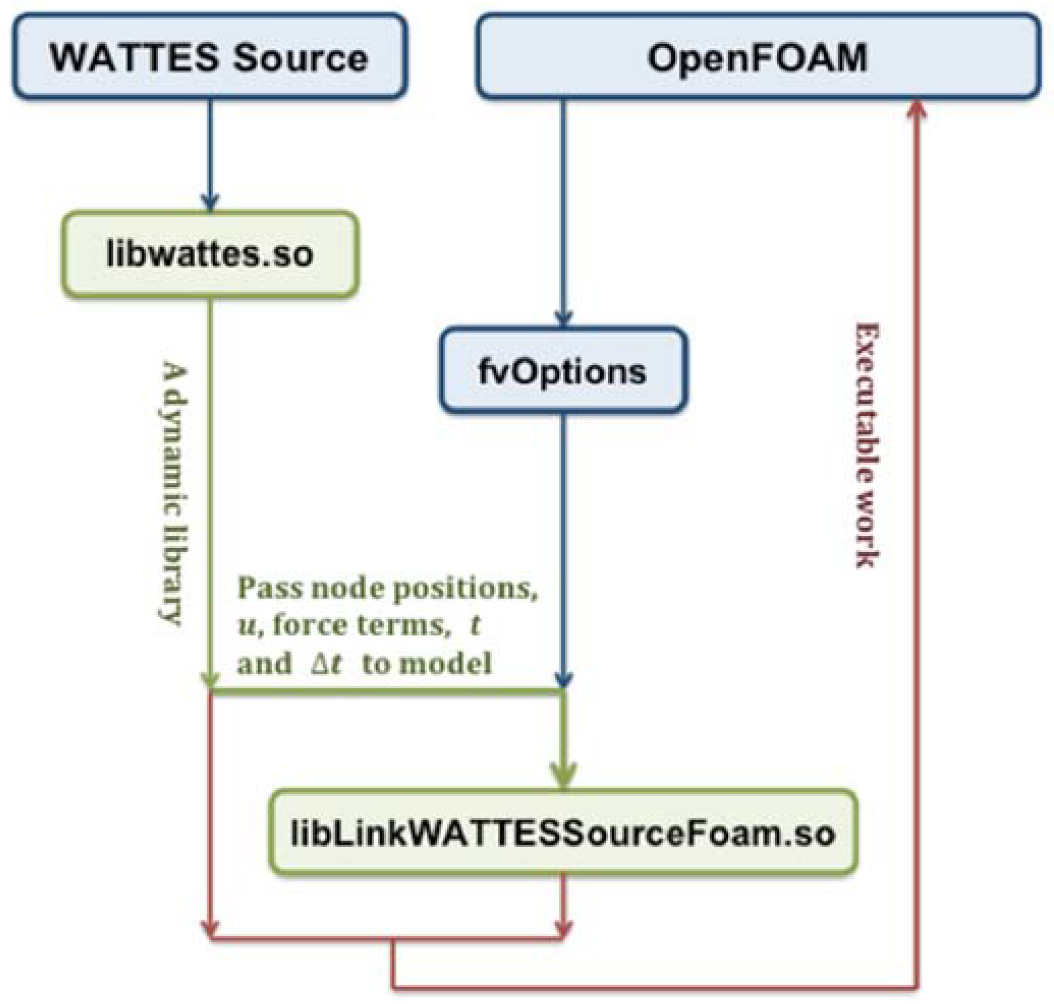
The Wind and Tidal Turbine Embedded Simulator (WATTES) [54,56] code is an open library source code written in Fortran 95, which employs both the dynamic torque-controlled actuator disc and the actuator line methods with active-pitch correction to simulate the behaviour of multiple wind and tidal horizontal-axis turbines, together with a simplified generator model. Compared with other momentum codes, WATTES predicts the dynamic response of the device to the flow, with lift and drag force components balanced by inertial effects and the resistive torque induced by the generator. Force components are incorporated within the incompressible Navier-Stokes momentum equations as body force components [54]. For computational efficiency, WATTES exploits parallel programming based on multiple instructions multiple data (MIMD) [52] through the Message Passaging Interface protocol (MPI). The solution is computed on a number of processors that function asynchronously and independently. The original WATTES model simulated flows using Fluidity, which is an open-source hr-adaptive multiphase computational fluid dynamics (CFD) solver based on an unstructured finite element method and offers anisotropic mesh refinement, developed mainly by researchers at Imperial College London [81]. The original WATTES source code was used to represent horizontal-axis turbines within the OpenFOAM [65] CFD framework, and formed the basis of the modified numerical model WATTES-V used herein to simulate flow past a vertical-axis turbine. OpenFOAM is freely available open-source CFD software based on the finite volume method on general unstructured polyhedral meshes, and is written in C++. In order to benefit from the advantages provided by the original WATTES source code, proper coupling of WATTES and OpenFOAM was a necessary prerequisite before the further development of WATTES-V model described in the present study.
The flow chart in Figure A1 summarises the coupled OpenFOAM-WATTES procedure. The main structure of OpenFOAM comprises four main directories: core OpenFOAM libraries (named src), solvers and utilities (applications), test cases that demonstrate a wide-range of OpenFOAM functionality (tutorials), and documentation (named doc). OpenFOAM is a collection of approximately 250 applications built upon a collection of over 100 software libraries (modules). Each application performs a specific task within a CFD workflow. Case setup is described by steering a collection of files in a tutorial directory, providing details of the mesh, physical models, solver, post-processing controls, etc. To couple the WATTES model with OpenFOAM, an interface program linking WATTES model was written in the src directory via a dynamic library with wrapper functions. The velocity field and momentum sources of the WATTES model were mapped to correspond correctly with those in OpenFOAM. A new fvOptions framework is introduced for run-time selectable physics by representing the force components from the WATTES model as momentum sources in the governing equations in OpenFOAM.
Figure A1. Flow chart of coupled OpenFOAM-WATTES program.
Energies 13 00776 g0a1

Appendix B

This Appendix presents results from tests which examine the influence of mesh convergence on the vorticity field in the near wake, the choice of inlet turbulence parameter, and the length of the downstream domain dimension.

Appendix B.1. Effect of Mesh Convergence on Near-Wake Vorticity Field

Figure A2 presents horizontal profiles of turbine mean streamwise velocity at a tip-speed ratio of 3.3 in the near-wake region computed on coarse, medium, and fine meshes (with N x = 150 , N x = 180 , and N x = 375 cells respectively in the x-direction). The figure illustrates model sensitivity to spatial resolution. Satisfactory agreement is generally achieved between the profiles obtained on the different meshes, although some slight discrepancies are evident, the relative two-norm errors [56] are 2.80 % , 2.44 % , 1.94 % respectively, which are all under 3 % and are within acceptable margins. We find that a spatial grid resolution of 150 cells in the x -direction, giving a total number of 6.72 × 10 5 cells in a 3D simulation, is sufficient to achieve mesh convergence.
Figure A2. Horizontal profiles computed on three meshes of normalised mean stream-wise velocity component at turbine mid-height where z / H   =   0 at (a) x = 0.5 D , (b) x = 1 D , and (c) x = 1.5 D .
Energies 13 00776 g0a2

Appendix B.2. Sensitivity Analysis concerning Inlet Turbulence Parameters
Turbulence intensity (TI) is defined as the ratio of the root-mean-square of flow velocity fluctuations u 1 3 ( u x 2 + u y 2 + u z 2 ) to the mean flow speed U U x 2 +   U y 2 + U z 2 [48], and is expressed:
TI u U = 2 3 · k U 2 ,
where k is turbulence kinetic energy (TKE). A value for TKE at the inlet is thus calculated from Equation (A1) for a given TI [82]. The specific dissipation rate ω used in the k - ω SST turbulence model in OpenFOAM is calculated using the following formula [83]:
ω = k 0.5 C μ l ,
where C μ is a turbulence model constant equal to 0.09 , and l is the turbulence length scale.
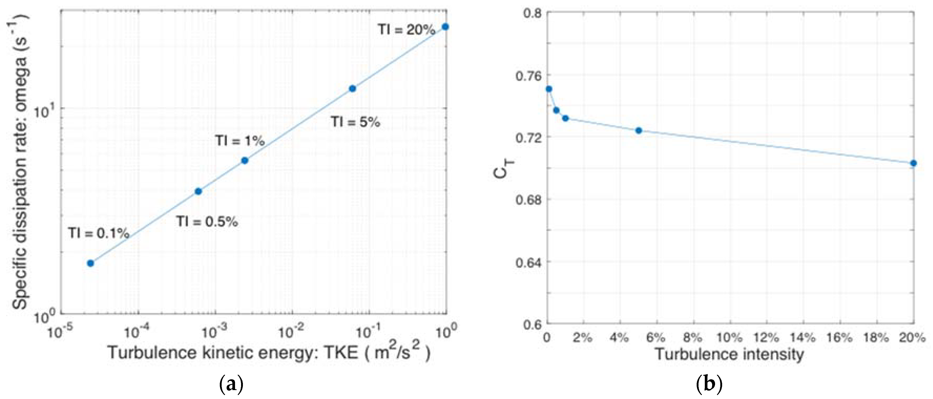
Sensitivity of the results to the inlet turbulence parameters is examined by setting different inlet values of k and ω calculated from Equations (A1) and (A2) for a range of turbulence intensity values from 0.1 % to 20 % , with TSR = 3.3 . The results are shown in Figure A3.
Figure A3. Inlet turbulence conditions and their effects on the vertical-axis turbine model for TI = 0.1 % , 0.5 % , 1 % , 5 % , and 20 % : (a) specific dissipation rate ( ω ) versus turbulence kinetic energy (TKE or k ), and (b) thrust coefficient versus TI.
Energies 13 00776 g0a3
Figure A3 displays the variation of specific dissipation rate with turbulence kinetic energy, and the thrust coefficient with turbulence intensity for the vertical-axis turbine model. It can be seen that the mean thrust coefficient tends to decrease as TI increases. In particular, as TI varies from 0.1 % to 20 % , the thrust coefficient decreases by 6.34 % . This indicates that the choice of level of turbulence intensity at the inlet can have a substantial effect on the thrust value of a vertical-axis turbine. However, the change of thrust coefficient is only about 1.72 % for a more realistic range of TI between 1 % and 10 % .

Appendix B.3. Sensitivity Analysis concerning Downstream Domain Size
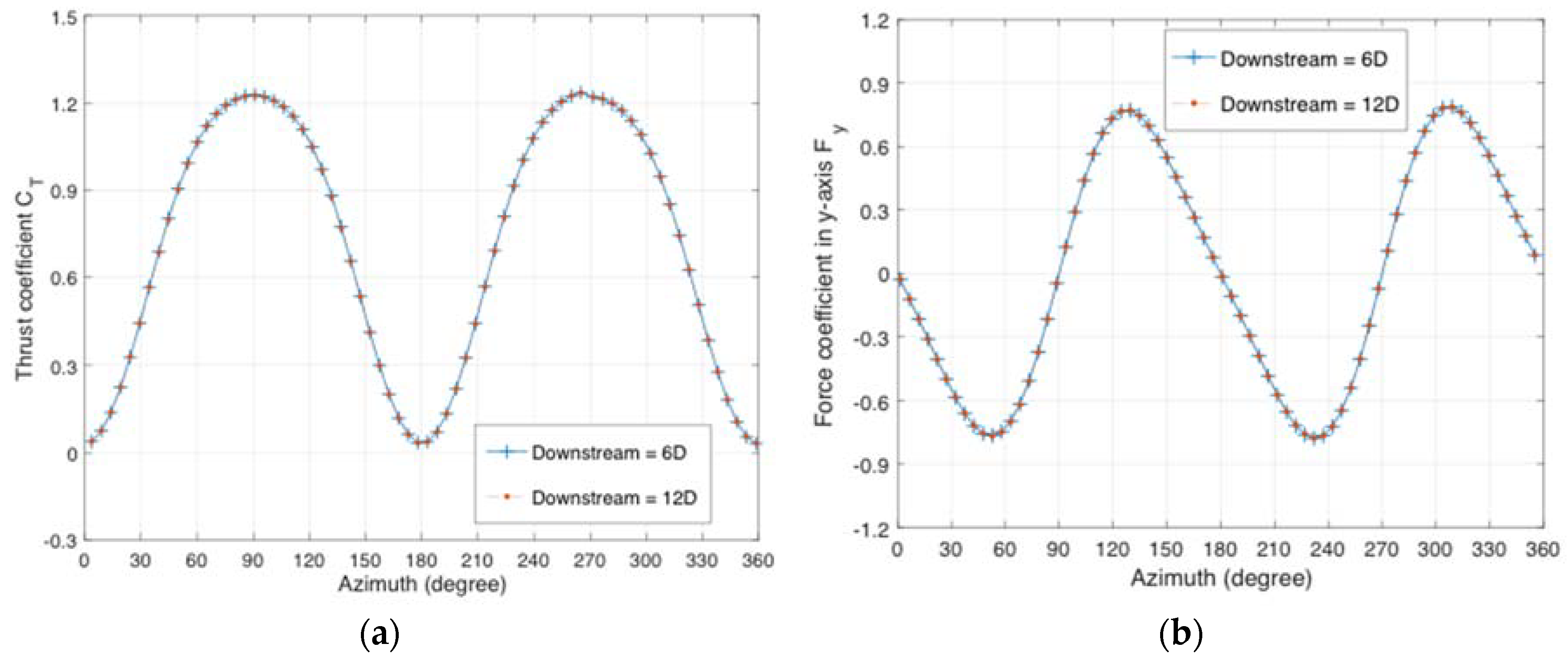
To investigate the impact of the limited downstream domain size on the results, we doubled the stream-wise length of the downstream domain, for a case of fixed TSR = 3.3 , and compared the thrust and lateral force coefficients obtained using the two domains.
Figure A4 shows that very satisfactory agreement is obtained for the values of C T and F y on the two domains, for a fixed TSR = 3.3; relative errors between the coefficients obtained using the different domains lie below 0.057 % . This confirms that the downstream length utilized in the main paper is adequate.
Figure A4. Comparison of predicted force coefficients obtained on meshes of downstream length 6 D and 12 D , for TSR = 3.3 as functions of azimuthal angle: (a) thrust coefficient C T ; and (b) lateral force coefficient F y .
Energies 13 00776 g0a4

References

  1. IEA. Energy and Climate Change; World Energy Outlook Special Report; IEA: Paris, France, 2015; Volume 479, pp. 1–200. [Google Scholar]
  2. EIA. International Energy Outlook 2017; U.S. Energy Information Administration, Office of Energy Analysis, US Department of Energy: Washington, DC, USA, 2017; p. 20585.
  3. Borthwick, A.G.L. Marine Renewable Energy Seascape. Engineering 2016, 2, 69–78. [Google Scholar] [CrossRef] [Green Version]
  4. International Energy Agency. Solutions for the 21st Century; International Energy Agency: Paris, France, 2002. [Google Scholar]
  5. Wong, K.H.; Chong, W.T.; Sukiman, N.L.; Poh, S.C.; Shiah, Y.-C.; Wang, C.-T. Performance enhancements on vertical axis wind turbines using flow augmentation systems: A review. Renew. Sustain. Rev. 2017, 73, 904–921. [Google Scholar] [CrossRef]
  6. Salter, S.H. Are nearly all tidal stream turbine designs wrong? In Proceedings of the 4th International Conference on Ocean Energy, Dublin, Ireland, 17–19 October 2012. [Google Scholar]
  7. Sutherland, H.J.; Berg, D.E.; Ashwill, T.D. A Retrospective of VAWT Technology; Technical Report, Sandia Report, SAND2012-0304; Sandia National Laboratories: Albuquerque, NM, USA, 2012.
  8. Strom, B.; Johnson, N.; Polagye, B. Impact of blade mounting structures on cross-flow turbine performance. J. Renew. Sustain. Energy 2018, 10, 034504. [Google Scholar] [CrossRef]
  9. Sahim, K.; Santoso, D.; Puspitasari, D. Investigations on the effect of radius rotor in combined Darrieus-Savonius wind turbine. Int. J. Rotating Mach. 2018, 2018, 3568542. [Google Scholar] [CrossRef] [Green Version]
  10. Subramanian, A.; Yogesh, S.A.; Sivanandan, H.; Giri, A.; Vasudevan, M.; Mugundhan, V.; Velamati, R.K. Effect of airfoil and solidity on performance of small scale vertical axis wind turbine using three dimensional CFD model. Energy 2017, 133, 179–190. [Google Scholar] [CrossRef]
  11. Dyachuk, E. Aerodynamics of Vertical-Axis Wind Turbines-Development of Simulation Tools and Experiments. Ph.D. Thesis, Uppsala University, Uppsala, Sweden, 2015. [Google Scholar]
  12. Salter, S.H.; Taylor, J.R.M. Vertical-axis tidal-current generators and the Pentland Firth. IMechE J. Power Energy 2006, 221, 181–199. [Google Scholar] [CrossRef]
  13. Suffera, K.H.; Usubamatovb, R.; Quadirc, G.A.; Ismaild, K. Modeling and numerical simulation of a vertical axis wind turbine having cavity vanes. In Proceedings of the 5th International Conference on Intelligent Systems, Modelling and Simulation, Langkawi, Malaysia, 27–29 January 2014. [Google Scholar]
  14. Dillmann, A.; Heller, G.; Klaas, M.; Kreplin, H.P.; Nitsche, W.; Schröder, W. New Results in Numerical and Experimental Fluid Mechanics VII; Contributions to the 16th STAB/DGLR Symposium Aachen, Germany; Springer: Berlin, Germany, 2008. [Google Scholar]
  15. Hameed, M.S.; Shahid, F. Evaluation of aerodynamic forces over a vertical axis wind turbine blade through CFD analysis. J. Appl. Mech. Eng. 2012. [Google Scholar] [CrossRef] [Green Version]
  16. Almohammadi, K.M.; Ingham, D.B.; Ma, L.; Pourkashanian, M. CFD sensitivity analysis of a straight-blade vertical axis wind turbine. Wind Eng. 2012, 36, 571–588. [Google Scholar] [CrossRef]
  17. Ghatage, S.V.; Joshi, J.B. Optimisation of vertical axis wind turbine: CFD simulations and experimental measurements. Can. J. Chem. Eng. 2012, 90, 1186–1201. [Google Scholar] [CrossRef]
  18. Zhang, L.X.; Liang, Y.B.; Liu, X.H.; Jiao, Q.F.; Guo, J. Aerodynamic performance prediction of straight-bladed vertical axis wind turbine based on CFD. Adv. Mech. Eng. 2013, 5, 905379. [Google Scholar] [CrossRef]
  19. Muneer, A.; Khan, M.B.; Sarwar, U.B.; Khan, Z.A.; Badar, M.S. CFD analysis of a Savonius Vertical axis wind turbine. In Proceedings of the 2015 Power Generation Systems and Renewable Energy Technologies, Islamabad, Pakistan, 10–11 June 2015. [Google Scholar]
  20. Asim, T.; Mishra, R.; Kaysthagir, S.; Aboufares, G. Performance comparison of a vertical axis wind turbine using commercial and open source computational fluid dynamics based codes. In Proceedings of the International Conference on Jets, Wakes and Separated Flows, Stockholm, Sweden, 16–18 June 2015. [Google Scholar]
  21. Alaimo, A.; Esposito, A.; Messineo, A.; Orlando, C.; Tumino, D. 3D CFD Analysis of a Vertical Axis Wind Turbine. Energies 2015, 8, 3013–3033. [Google Scholar] [CrossRef] [Green Version]
  22. Bai, C.J.; Lin, Y.Y.; Lin, S.Y.; Wang, W.C. Computational fluid dynamics analysis of the vertical axis wind turbine blade with tubercle leading edge. J. Renew. Sustain. Energy 2015, 7, 033124. [Google Scholar] [CrossRef]
  23. Rezaeiha, A.; Kalkman, I.; Blocken, B. CFD simulation of a vertical axis wind turbine operating at a moderate tip speed ratio: Guidelines for minimum domain size and azimuthal increment. Renew. Energy 2017, 107, 373–385. [Google Scholar] [CrossRef] [Green Version]
  24. Unsakul, S.; Sranpat, C.; Chaisiriroj, P.; Leephakpreeda, T. CFD-based performance analysis and experimental investigation of design factors of vertical axis wind turbines under low wind speed conditions in Thailand. J. Flow Control Meas. Vis. 2017, 5, 86–98. [Google Scholar] [CrossRef] [Green Version]
  25. Naccache, G.; Paraschivoiu, M. Development of the dual vertical axis wind turbine using computational fluid dynamics. J. Fluids Eng. 2017, 139, 121105. [Google Scholar] [CrossRef]
  26. Kao, J.H.; Tseng, P.Y. Application of computational fluid dynamics (CFD) simulation in a vertical axis wind turbine (VAWT) system. IOP Conf. Ser. Earth Environ. 2018, 114, 012002. [Google Scholar] [CrossRef]
  27. Li, C.; Xiao, Y.; Xu, Y.; Peng, Y.; Hu, G.; Zhu, S. Optimization of blade pitch in H-rotor vertical axis wind turbines through computational fluid dynamics simulations. Appl. Energy 2018, 212, 1107–1125. [Google Scholar] [CrossRef]
  28. Gokulnath, R.; Devi, P.B.; Senbagan, M.; Manigandan, S. CFD analysis of Savonious type vertical axis wind turbine. IJMET 2018, 9, 1378–1383. [Google Scholar]
  29. Elsakka, M.M.; Ingham, D.; Ma, L.; Pourkashanian, M. CFD analysis of the angle of attack for a vertical axis wind turbine blade. Energy Convers. Manag. 2019, 182, 154–165. [Google Scholar] [CrossRef]
  30. Bachant, P.; Goude, A.; Wosnik, M. Actuator line modelling of vertical-axis turbines. arXiv 2018, arXiv:1605.01449v4. [Google Scholar]
  31. Burton, T.; Jenkins, N.; Sharpe, D.; Bossanyi, E. Wind Energy Handbook, 2nd ed.; Wiley: Hoboken, NJ, USA, 2011. [Google Scholar]
  32. Okpue, A.S. Aerodynamic Analysis of Vertical and Horizontal Axis Wind Turbines. Master’s Thesis, Michigan State University, East Lansing, MI, USA, 2011. [Google Scholar]
  33. Shires, A. Development and Evaluation of an Aerodynamic Model for a Novel Vertical Axis Wind Turbine Concept. Energies 2013, 6, 2501–2520. [Google Scholar] [CrossRef] [Green Version]
  34. Bianchini, A.; Balduzzi, F.; Haack, L.; Bigalli, S.; Müller, B.; Ferrara, G. Development and Validation of a Hybrid Simulation Model for Darrieus Vertical-Axis Wind Turbines. In Proceedings of the ASME Turbo Expo 2019: Turbomachinery Technical Conference and Exposition GT2019-91218, Phoenix, AZ, USA, 17–21 June 2019. [Google Scholar]
  35. Mikkelsen, R.F. Actuator Disc Methods Applied to Wind Turbines. Ph.D. Thesis, MEK-FM-PHD, No. 2003-02. Technical University of Denmark, Lyngby, Denmark, 2004. [Google Scholar]
  36. Newman, B.G. Actuator-disc theory for vertical-axis wind turbines. J. Wind Eng. Ind. Aerodyn. 1983, 15, 347–355. [Google Scholar] [CrossRef]
  37. Linton, D.; Barakos, G.; Widjaja, R.; Thornbern, B. A new actuator surface model with improved wake model for CFD simulations of rotorcraft. In Proceedings of the 73rd Annual Forum and Technology Display of the American Helicopter Society, Fort Worth, TX, USA, 9–11 May 2017. [Google Scholar]
  38. Shen, W.; Zhang, J.; Sorensen, J. The actuator surface model: A new Navier-Stokes based model for rotor computations. J. Sol. Energy Eng. 2009, 131, 011002. [Google Scholar] [CrossRef]
  39. Massie, L.; Ouro, P.; Stoesser, T.; Luo, Q. An Actuator Surface Model to Simulate Vertical Axis Turbines. Energies 2019, 12, 4741. [Google Scholar] [CrossRef] [Green Version]
  40. Bachant, P.; Wosnik, M. Characterising the near-wake of a cross-flow turbine. J. Turbul. 2015, 16, 392–410. [Google Scholar] [CrossRef]
  41. Riva, L.; Giljarhus, K.E.; Hjertager, B.; Kalvig, S.M. Implementation and application of the actuator line model by OpenFOAM for a vertical axis wind turbine. IOP Conf. Ser. Mater. Sci. Eng. 2017, 276, 012002. [Google Scholar] [CrossRef]
  42. Sørensen, J.N.; Shen, W.Z. Numerical modelling of wind turbine wakes. J. Fluids Eng. 2002, 124, 393–399. [Google Scholar] [CrossRef]
  43. Troldborg, N. Actuator Line Modelling of Wind Turbine Wakes. Ph.D. Thesis, Technical University of Denmark, Lyngby, Denmark, June 2008. [Google Scholar]
  44. Martinez, L.; Leonardi, S.; Churchfield, M.; Moriarty, P. A comparison of actuator disk and actuator line wind turbine models and best practices for their use. AIAA J. 2012, 16. [Google Scholar] [CrossRef]
  45. Shamsoddin, S.; Porté-Agel, F. Large Eddy Simulation of vertical axis wind turbine wakes. Energies 2014, 7, 890–912. [Google Scholar] [CrossRef]
  46. Reynolds, O. On the dynamical theory of incompressible viscous fluids and the determination of the criterion. Philos. Trans. R. Soc. Lond. A 1895, 186, 123–164. [Google Scholar]
  47. Hanjalic, K.; Launder, B. A Reynolds stress model of turbulence and its application to thin shear flows. J. Fluid Mech. 1972, 52, 609–638. [Google Scholar] [CrossRef]
  48. Wilcox, D.C. Turbulence Modelling for CFD, 2nd ed.; DCW Industries Inc.: La Canada, CA, USA, 1998. [Google Scholar]
  49. Wilcox, D.C. Formulation of the k-omega Turbulence Model Revisited. AIAA J. 2008, 46, 11. [Google Scholar] [CrossRef] [Green Version]
  50. Deardorff, J. A numerical study of three-dimensional turbulent channel flow at large Reynolds numbers. J. Fluid Mech. 1970, 41, 453–480. [Google Scholar] [CrossRef]
  51. Smagorinsky, J. General Circulation Experiments with the Primitive Equation. Mon. Weather Rev. 1963, 91, 99. [Google Scholar] [CrossRef]
  52. Creech, A.C.W. A Three-Dimensional Numerical Model of a Horizontal Axis, Energy Extracting Turbine. Ph.D. Thesis, Heriot-Watt University, Edinburgh, Scotland, UK, March 2009. [Google Scholar]
  53. Creech, A.; Früh, W.-G.; Clive, P. Actuator volumes and hr-adaptive methods for three-dimensional simulation of wind turbine wakes and performance. Wind Energy 2011, 15, 847–863. [Google Scholar] [CrossRef]
  54. Creech, A.C.W.; Früh, W.G.; Maguire, A.E. Simulations of an offshore wind farm using large eddy simulation and a torque-controlled actuator disc model. Surv. Geophys. 2015, 36, 427–481. [Google Scholar] [CrossRef] [Green Version]
  55. Creech, A.; Früh, W.-G. Modelling wind turbine wakes for wind farms. In Alternative Energy and Shale Gas Encyclopedia; Lehr, J., Keeley, J., Eds.; The University of Edinburgh: Edinburgh, UK, 2016. [Google Scholar]
  56. Creech, A.C.W.; Borthwick, A.G.L.; Ingram, D. Effects of support structures in an LES actuator line model of a tidal turbine with contra-rotating rotors. Energies 2017, 10, 726. [Google Scholar] [CrossRef] [Green Version]
  57. McLaren, K.W. Unsteady Loading of High Solidity Vertical Axis Wind Turbines. Ph.D. Thesis, McMaster University, Hamilton, ON, Canada, 2011. [Google Scholar]
  58. Nobile, R.; Vahdati, M.; Barlow, J.F. Unsteady flow simulation of a vertical axis wind turbine: A two-dimensional study. J. Wind Eng. Ind. Aerodyn. 2014, 125, 168–179. [Google Scholar] [CrossRef] [Green Version]
  59. Biadgo, A.M.; Simonovic, A.; Komarov, D.; Stupar, S. Numerical and analytical investigation of vertical axis wind turbine. FME Trans. 2013, 41, 49–58. [Google Scholar]
  60. Bachant, P.; Wosnik, M. Modelling the near-wake of a vertical-axis cross-flow turbine with 2-D and 3-D RANS. J. Renew. Sustain. Energy 2016, 8, 053311. [Google Scholar] [CrossRef] [Green Version]
  61. Krogstad, P.A.; Eriksen, P.E. Blind test calculations of the performance and wake development for a model wind turbine. Renew. Energy 2013, 50, 325–333. [Google Scholar] [CrossRef]
  62. Buntine, J.D.; Pullin, D.I. Merger and cancellation of strained vortices. J. Fluid Mech. 1989, 205, 263–295. [Google Scholar] [CrossRef] [Green Version]
  63. Rezaeiha, A.; Kalkman, I.; Blocken, B. Effect of pitch angle on power performance and aerodynamics of a vertical axis wind turbine. Appl. Energy 2017, 197, 132–150. [Google Scholar] [CrossRef] [Green Version]
  64. Hwang, I.S.; Lee, Y.H.; Kim, S.J. Optimization of cycloidal water turbine and the performance improvement by individual blade control. Appl. Energy 2009, 86, 1532–1540. [Google Scholar] [CrossRef]
  65. Zhao, R.; Creech, A.C.W.; Borthwick, A.G.L.; Nishino, T. Coupling of WATTES and OpenFOAM codes for wake modelling behind close-packed contra-rotating vertical-axis tidal rotors. In Proceedings of the 6th Oxford Tidal Energy Workshop, Oxford, UK, 26–27 March 2018. [Google Scholar]
  66. Schito, P.; Zasso, A. Actuator forces in CFD: RANS and les modelling in OpenFOAM. J. Phys. Conf. Ser. 2014, 524, 012160. [Google Scholar] [CrossRef]
  67. Jha, P.K.; Churchfield, M.J.; Moriarty, P.J.; Schmitz, S. Guidelines for volume force distributions within actuator line modelling of wind turbines on large-eddy simulation-type grids. J. Sol. Energy Eng. 2014, 136, 031003. [Google Scholar] [CrossRef]
  68. Martínez-Tossas, L.A.; Churchfield, M.J.; Meneveau, C. Optimal smoothing length scale for actuator line models of wind turbine blades. Wind Energy 2015, 20, 1083–1096. [Google Scholar] [CrossRef]
  69. Tennekes, H.; Lumley, J.L. A First Course in Turbulence; The MIT Press: Cambridge, MA, USA, 1972. [Google Scholar]
  70. LeBlanc, B.P.; Ferreira, C.S. Experimental determination of thrust loading of a 2-bladed vertical axis wind turbine. J. Phys. Conf. Ser. 2018, 1037, 022043. [Google Scholar] [CrossRef] [Green Version]
  71. Menter, F.R. Two-Equation Eddy-Viscosity Turbulence Models for Engineering Applications. AIAA J. 1994, 32, 8. [Google Scholar] [CrossRef] [Green Version]
  72. Barthelmie, R.J.; Hansen, K.; Frandsen, S.T.; Rathmann, O.; Schepers, J.G.; Schlez, W.; Phillips, J.; Rados, K.; Zervos, A.; Politis, E.S.; et al. Modelling and measuring flow and wind turbine wakes in large wind farms offshore. Wind Energy 2009, 12, 431–444. [Google Scholar] [CrossRef]
  73. Bachant, P. Physical and numerical modeling of cross-flow turbines. Ph.D. Thesis, University of New Hampshire, Durham, NC, USA, 2016. [Google Scholar]
  74. Roache, P.J. Perspective: A method for uniform reporting of grid refinement studies. J Fluid Eng. ASME 1994, 116, 405–413. [Google Scholar] [CrossRef]
  75. Bakhvalov, N.S. Courant–Friedrichs–Lewy condition. In Encyclopedia of Mathematics; Michiel, H., Ed.; Springer Science + Business Media, B.V./Kluwer Academic Publishers: Berlin, Germany, 2001; ISBN 978-1-55608-010-4. [Google Scholar]
  76. Sheldahl, R.E.; Klimas, P.C. Aerodynamic Characteristics of Seven Symmetrical Airfoil Sections through 180-Degree Angle of Attack for Use in Aerodynamic Analysis of Vertical Axis Wind Turbines; Energy Report; Sandia National Lab: Albuquerque, NM, USA, 1981.
  77. Ouro, P.; Stoesser, T. An immersed boundary-based large-eddy simulation approach to predict the performance of vertical axis tidal turbines. Comput. Fluids 2017, 152, 74–87. [Google Scholar] [CrossRef] [Green Version]
  78. Brochier, G.; Fraunie, P.; Beguier, C.; Paraschivoiu, I. Water channel experiments of dynamic stall on Darrieus wind turbine blades. J. Propuls. Power 1986, 2, 445–449. [Google Scholar] [CrossRef]
  79. Araya, D.B.; Dabiri, J.O. A comparison of wake measurements in motor-driven and flow-driven turbine experiments. Exp. Fluids 2015, 56, 150. [Google Scholar] [CrossRef]
  80. Ouro, P.; Runge, S.; Luo, Q.; Stoesser, T. Three-dimensionality of the wake recovery behind a vertical axis turbine. Renew. Energy 2018, 133, 1066–1077. [Google Scholar] [CrossRef] [Green Version]
  81. Piggott, M.; Pain, C.; Gorman, G.; Power, P.; Goddard, A. h, r, and hr adaptivity with applications in numerical ocean modelling. Ocean Model 2004, 10, 95–113. [Google Scholar] [CrossRef]
  82. Jensen, B.B.B. Numerical study of influence of inlet turbulence parameters on turbulence intensity in the flow domain: Incompressible flow in pipe system. Proc. IMechE Part E J. Process Mech. Eng. 2007, 221, 177–185. [Google Scholar] [CrossRef]
  83. User Guide: K-Omega Shear Stress Transport (SST)—OpenFOAM. Available online: https://www.openfoam.com/documentation/guides/latest/doc/guide-turbulence-ras-k-omega-sst.html (accessed on 2 February 2020).
Figure 1. Artist’s impression of close-packed vertical-axis contra-rotating rotors [12].
Energies 13 00776 g001
Figure 2. Geometry of and force vectors on a blade of a rotating vertical-axis turbine (VAT). The flow velocity relative to the blades is u r e l ; the angle of attack α is calculated from the local inflow velocity u ; the freestream velocity u 0 ; and the blade velocity is u b l . The azimuthal blade angle is θ with the corrected blade pitch β ; and θ r e l is relative angle. F L and F D are lift and drag forces per unit span respectively for the actuator line.
Energies 13 00776 g002
Figure 3. Computational mesh and boundary conditions, showing plan dimensions of the modelled domain.
Energies 13 00776 g003
Figure 4. Resolution sensitivity of the VAT model: (a) Spatial resolution after 120 time steps per revolution; (b) Temporal resolution on a mesh with 150 cells in x-direction.
Energies 13 00776 g004
Figure 5. Comparison between predicted and measured [70] thrust and lateral forces on a wind turbine rotor of a two-bladed H-type vertical-axis wind turbine for an incoming flow speed of 4.01   m / s , fixed pitch blade angle of 0 ° , and tip speed ratio of 3.7 .
Energies 13 00776 g005
Figure 6. Comparison between predicted and measured [70] mean thrust coefficient C T as a function of tip speed ratio in the range from 2.7 to 3.7 , for a wind turbine rotor of a two-bladed H-type vertical-axis wind turbine with incoming flow speed of 4.01   m / s and fixed pitch blade angle of 0 ° .
Energies 13 00776 g006
Figure 7. Comparison between predicted and measured [70] thrust and lateral force coefficients for different values of tip-speed ratio (TSR) ( 2.9 , 3.3 , and 3.7 ) as functions of azimuthal angle: (a) Thrust coefficient C T ; and (b) Lateral force coefficient F y .
Energies 13 00776 g007
Figure 8. Lift coefficient as a function of local angle of attack at each grid point predicted by the VAT model for TSR = 2.9 , compared with measurements for a static airfoil [76]; the red dashed lines show the range of local angle of attack.
Energies 13 00776 g008
Figure 9. Flow patterns at eight different phases during a single revolution for TSR = 3.7 : (a) Velocity magnitude ( m / s ); (b) z -component of vorticity ( s 1 ); and (c) Turbulence kinetic energy ( m 2 / s 2 ) in the central horizontal x - y plane.
Energies 13 00776 g009
Figure 10. Snapshot of vorticity iso-surfaces, coloured according to z -component.
Energies 13 00776 g010
Figure 11. Variance of angle of attack as a function of azimuthal angle at TSR = 3.7 .
Energies 13 00776 g011
Figure 12. Near wake flow at x / D   =   1 and z / H   =   0 : (a) Slices through the mean velocity field in the y - z and x - y planes at TSR = 3.7 ; (b) Slices through the mean turbulence kinetic energy contours at TSR = 3.7 ; (c) Mean stream-wise velocity profiles for TSR =   2.9 , 3.3 , and 3.7 ; and (d) Mean turbulence kinetic energy profiles for TSR =   2.9 , 3.3 , and 3.7 .
Energies 13 00776 g012
Figure 13. Horizontal profiles at mid-elevation of turbine z / H   =   0 : mean stream-wise velocity component (a) TSR = 2.9 , (b) TSR = 3.3 , (c) TSR = 3.7 ; and turbulence kinetic energy (d) TSR = 2.9 , (e) TSR = 3.3 , (f) TSR = 3.7 .
Energies 13 00776 g013
Figure 14. Variation of angular velocity ω as a function of azimuthal angle in the torque-controlled system at TSR = 3.3 .
Energies 13 00776 g014
Figure 15. Variation of torque coefficient C Q as a function of azimuthal angle at TSR = 3.3 : (a) Comparison between results from the model with fixed TSR and its torque-controlled counterpart; (b) Enlarged zone of C Q variation in the torque-controlled model.
Energies 13 00776 g015
Figure 16. Comparison between predicted (including the model with fixed TSR and the torque-controlled model) and measured [70] thrust and lateral force coefficients for TSR = 3.3 as functions of azimuthal angle: (a) thrust coefficient C T ; and (b) lateral force coefficient F y .
Energies 13 00776 g016
Table 1. VAT model parameters based on the experimental turbine configuration at Delft [70].
PropertySymbolValue/Dimension
Number of blades N b l 2
Turbine diameter D 1.48   m
Blade length L 1.5   m
Aerofoil type NACA   0021
Chord c 0.075   m
Blade pitch β p 0 °
Freestream flow speed u 0 4.01   m / s
Fluid density ρ 1.207   kg / m 3
Local Reynolds number R e c 19 , 838