Numerical Modeling of Bifacial PV String Performance: Perimeter Effect and Influence of Uniaxial Solar Trackers


Abstract
:1. Introduction
2. Methods and Model Description
3. Results and Discussion
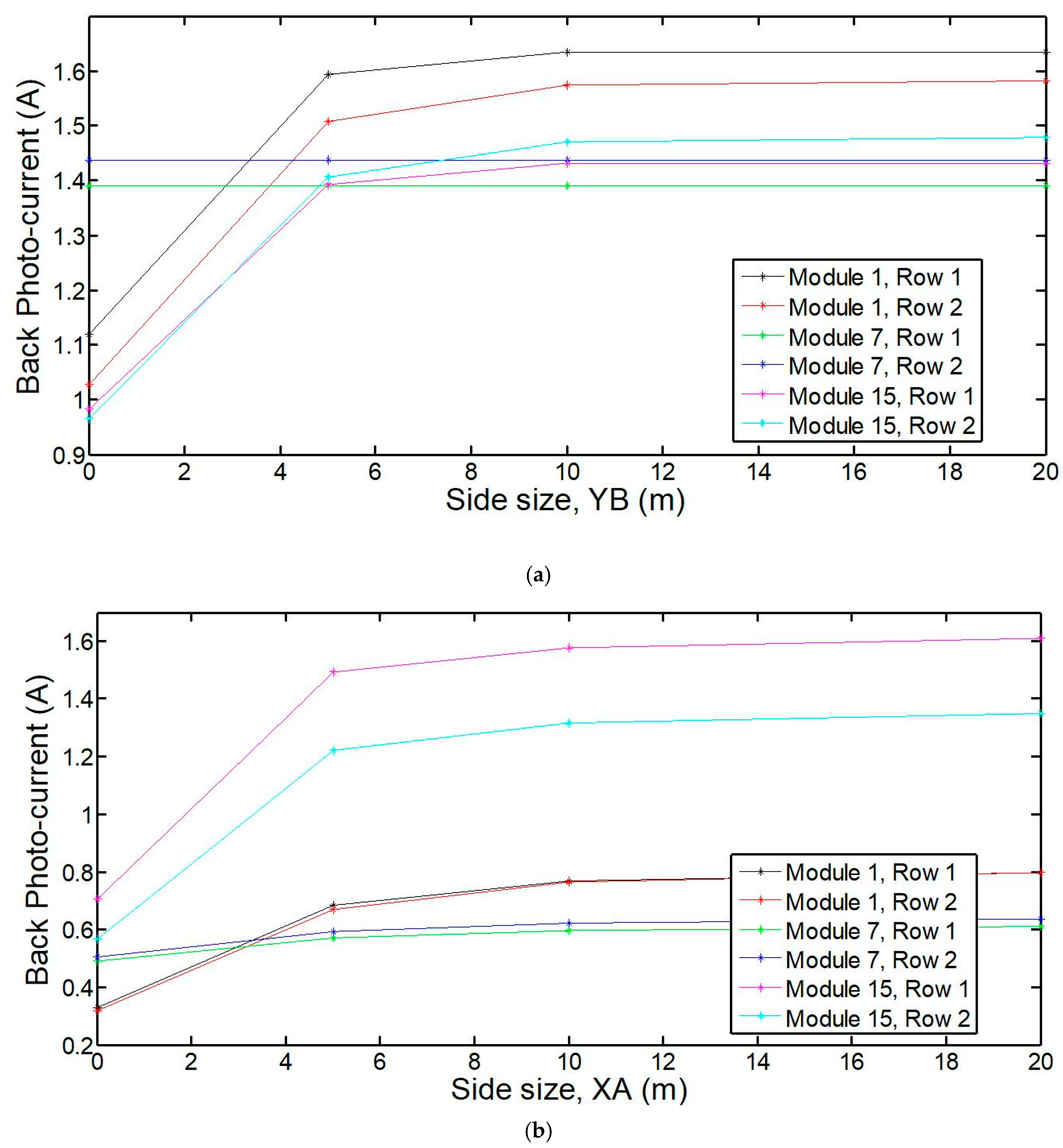
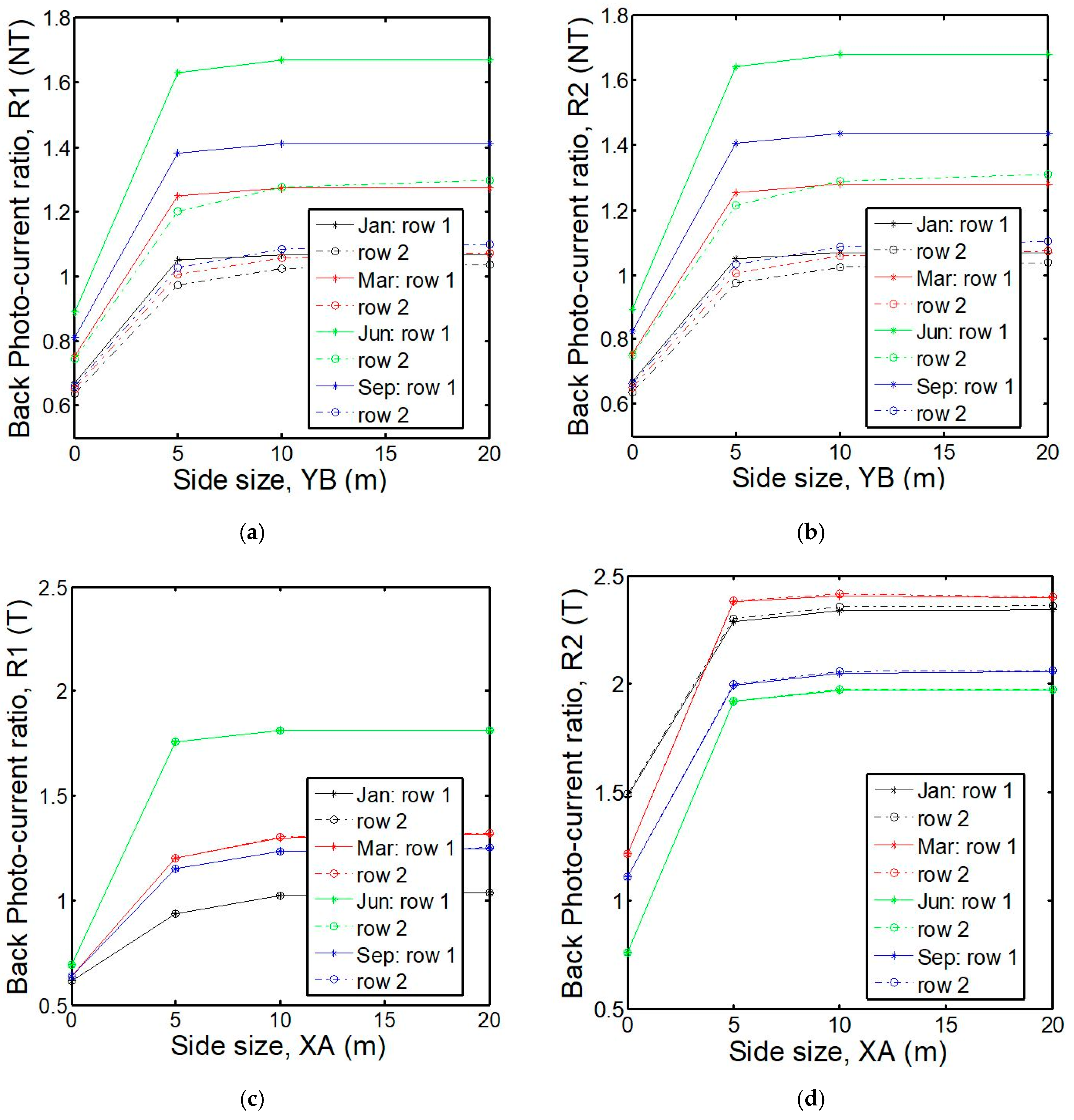
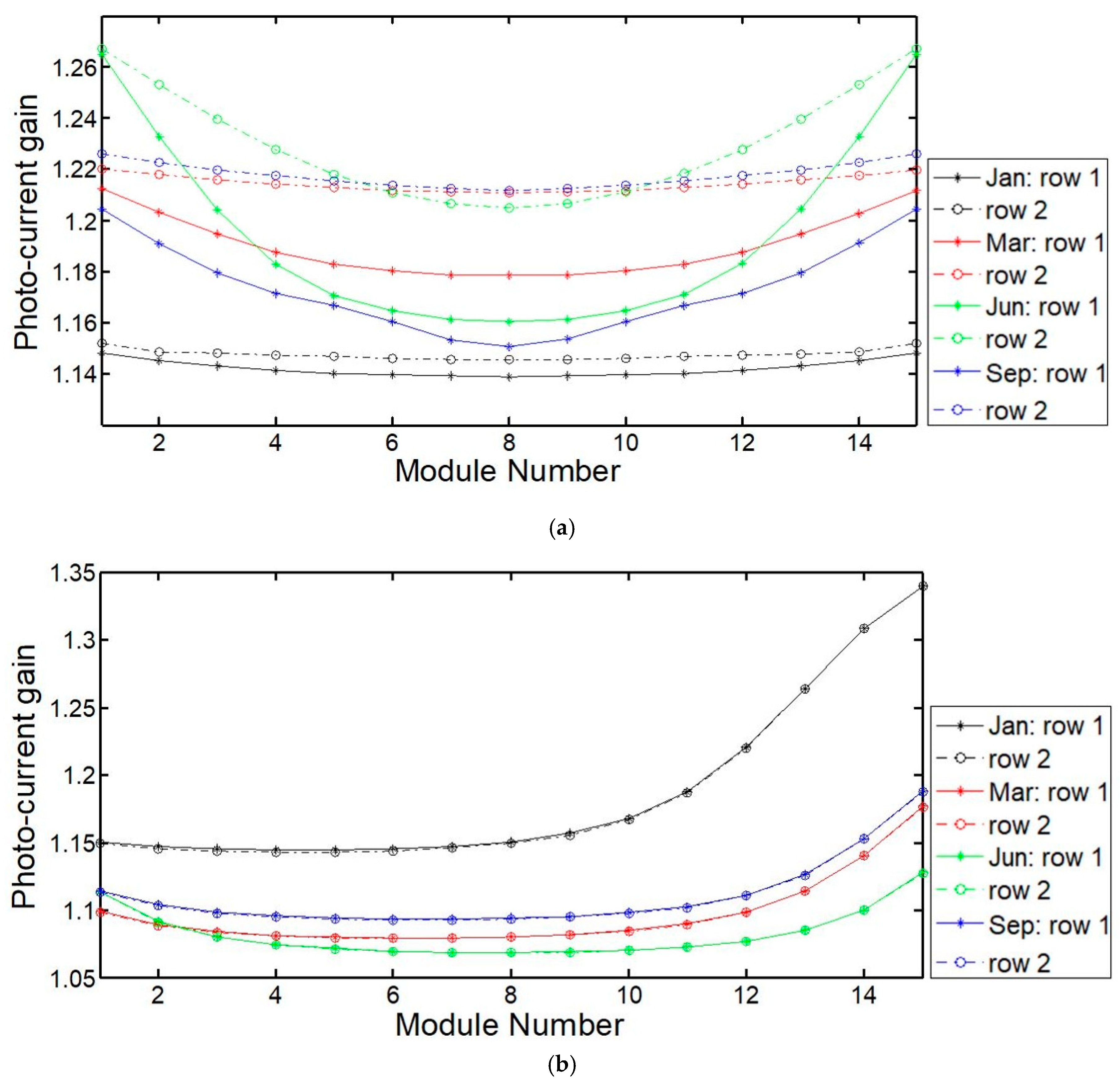
3.1. Perimeter Effects
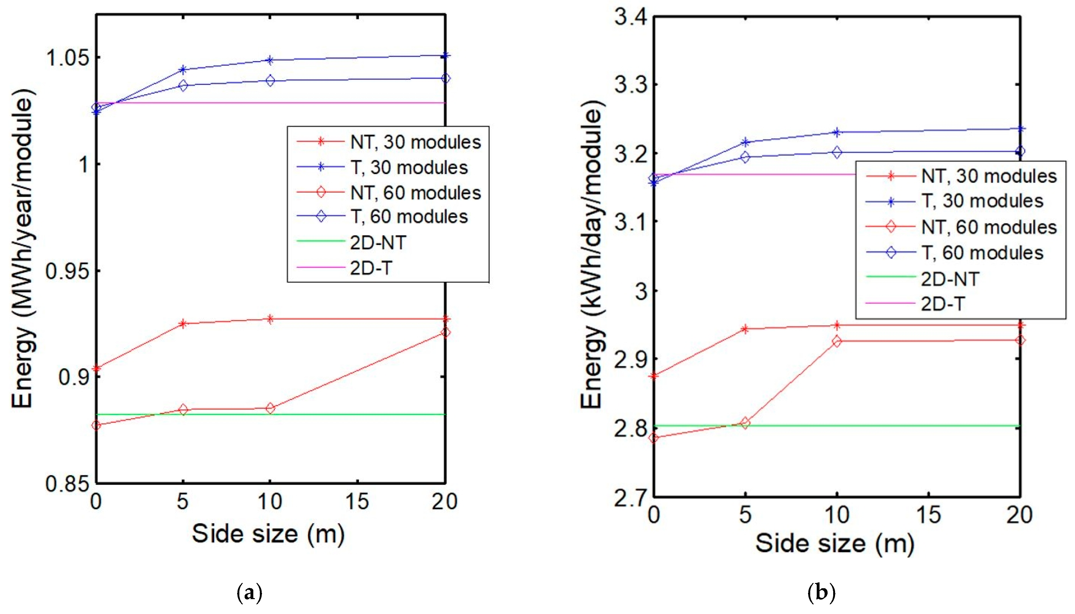
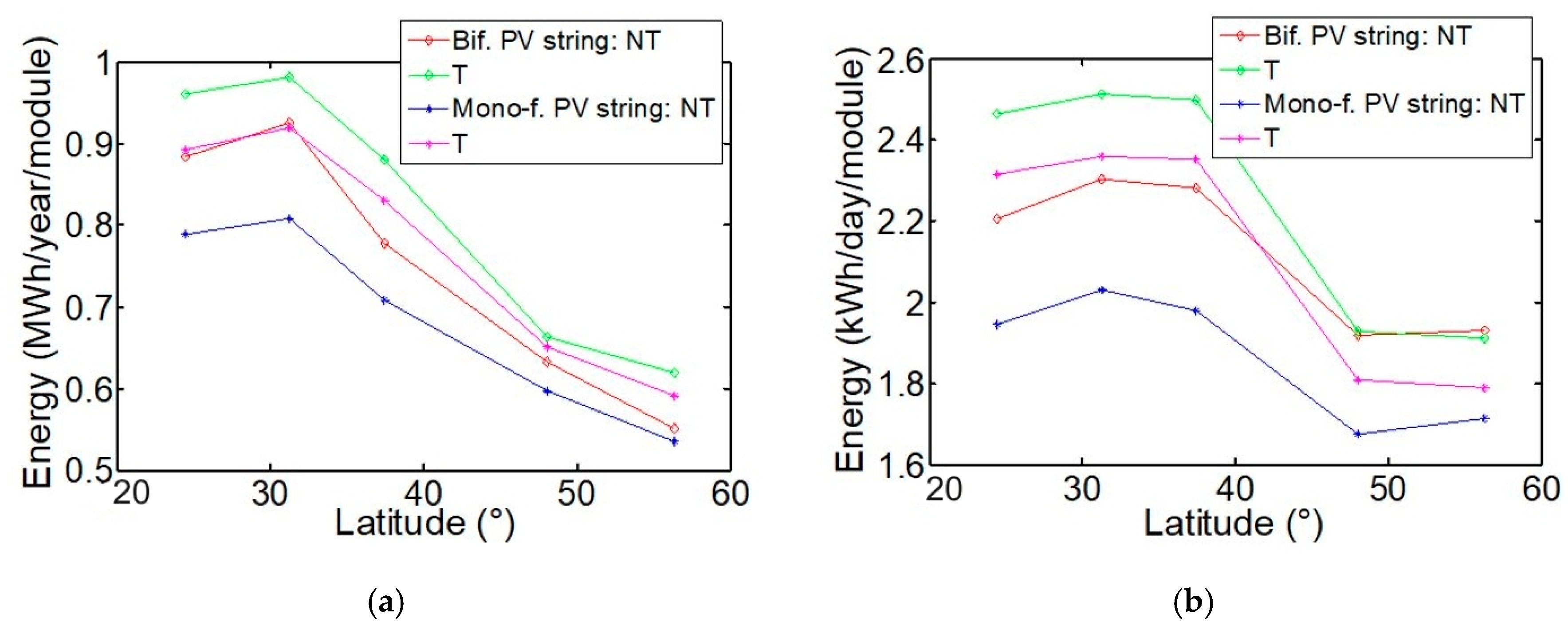
3.2. Latitude Effect
4. Conclusions
Author Contributions
Funding
Conflicts of Interest
References
- Pujari N, S.; Cellere, G.; Falcon, T.; Hage, F.; Zwegers, M.; Bernreuter, J.; Haase, J.; Yakovlev, S.; Coletti, G.; Romijn, I.; et al. International Technology Roadmap for Photovoltaic (ITRPV) Results 2017 Including Maturity Report 2018 Ninth Edition, September 2018 ITRPV. 2018. Available online: https://pv.vdma.org/en/ (accessed on 16 February 2020).
- Yusufoglu, U.A.; Lee, T.H.; Pletzer, T.; Halm, A.; Koduvelikulathu, L.; Comparotto, C.; Kopecek, R.; Kurz, H. Simulation of Energy Production by Bifacial Modules with Revision of Ground Reflection. Energy Procedia 2014, 55. [Google Scholar] [CrossRef] [Green Version]
- Yusufoglu, U.A.; Pletzer, T.M.; Koduvelikulathu, L.J.; Comparotto, C.; Kopecek, R.; Kurz, H. Analysis of the Annual Performance of Bifacial Modules and Optimization Methods. IEEE J. Photovolt. 2015, 5, 320–328. [Google Scholar] [CrossRef]
- Shoukry, I.; Libal, J.; Kopecek, R.; Wefringhaus, E.; Werner, J. Modelling of Bifacial Gain for Stand-alone and in-field Installed Bifacial PV Modules. Energy Procedia 2016, 92, 600–608. [Google Scholar] [CrossRef] [Green Version]
- Appelbaum, J. Bifacial photovoltaic panels field. Renew. Energy 2016, 85, 338–343. [Google Scholar] [CrossRef]
- Hansen, C.W.; Riley, D.M.; Deline, C.; Toor, F.; Stein, J.S. A Detailed Performance Model for Bifacial PV Modules. In Proceedings of the 33rd European Photovoltaic Solar Energy Conference and Exhibition, Amsterdam, The Netherlands, 25–29 September 2017. [Google Scholar] [CrossRef]
- Deline, C.; MacAlpine, S.; Marion, B.; Toor, F.; Asgharzadeh, A.; Stein, J.S. Assessment of Bifacial Photovoltaic Module Power Rating Methodologies—Inside and Out. IEEE J. Photovolt. 2017, 7, 575–580. [Google Scholar] [CrossRef]
- Sun, X.; Khan, M.R.; Deline, C.; Alam, M.A. Optimization and performance of bifacial solar modules: A global perspective. Appl. Energy 2018, 212, 1601–1610. [Google Scholar] [CrossRef] [Green Version]
- Chudinzow, D.; Haas, J.; Díaz-Ferrán, G.; Moreno-Leiva, S.; Eltrop, L. Simulating the energy yield of a bifacial photovoltaic power plant. Sol. Energy 2019, 183, 812–822. [Google Scholar] [CrossRef]
- Ricco Galluzzo, F.; Canino, A.; Gerardi, C.; Lombardo, S.A. A new model for predicting bifacial PV modules performance: First validation results. In Proceedings of the 46th IEEE Photovoltaic Specialists Conference (PVSC 46), Chicago, IL, USA, 16–21 June 2019. [Google Scholar]
- Katsaounis, T.; Kotsovos, K.; Gereige, I.; Al-Saggaf, A.; Tzavaras, A. 2D simulation and performance evaluation of bifacial rear local contact c-Si solar cells under variable illumination conditions. Sol. Energy 2017, 158, 34–41. [Google Scholar] [CrossRef] [Green Version]
- Katsaounis, T.; Kotsovos, K.; Gereige, I.; Basaheeh, A.; Abdullah, M.; Khayat, A.; Al-Habshi, E.; Al-Saggaf, A.; Tzavaras, A.E. Performance assessment of bifacial c-Si PV modules through device simulations and outdoor measurements. Renew. Energy 2019, 143, 1285–1298. [Google Scholar] [CrossRef]
- Pvsyst Photovoltaic Software. Available online: https://www.pvsyst.com/help/bifacial_systems.htm (accessed on 16 February 2020).
- Cai, W.; Yuan, S.; Sheng, Y.; Duan, W.; Wang, Z.; Chen, Y.; Yang, Y.; Pietro, P.; Altermatt, P.P.; Verlinden, P.J.; et al. 22.2% efficiency n-type PERT solar cell. Energy Procedia 2016, 92, 399–403. [Google Scholar] [CrossRef] [Green Version]
- Neville, R.C. Solar energy collector orientation and tracking mode. Sol. Energy 1978, 20, 7–11. [Google Scholar] [CrossRef]
- Nann, S. Potentials for tracking photovoltaic systems and V-troughs in moderate climates. Sol. Energy 1990, 45, 385–393. [Google Scholar] [CrossRef]
- Poulek, V.; Libra, M. New solar tracker. Sol. Energy Mater. Sol. Cells 1998, 51, 113–120. [Google Scholar] [CrossRef]
- Lorenzo, E.; Pérez, M.; Ezpeleta, A.; Acedo, J. Design of tracking photovoltaic systems with a single vertical axis. Prog. Photovolt. 2002, 10, 533–543. [Google Scholar] [CrossRef]
- Abdallah, S. The effect of using sun tracking systems on the voltage–current characteristics and power generation of flat plate photovoltaics. Energy Convers. Manag. 2004, 45, 1671–1679. [Google Scholar] [CrossRef]
- Al-Mohamad, A. Efficiency improvements of photo-voltaic panels using a Sun-tracking system. Appl. Energy 2004, 79, 345–354. [Google Scholar] [CrossRef]
- Bione, J.; Vilela, O.C.; Fraidenraich, N. Comparison of the performance of PV water pumping systems driven by fixed, tracking and V-trough generators. Sol. Energy 2004, 76, 703–711. [Google Scholar] [CrossRef]
- Karimov, K.S.; Saqib, M.A.; Akhter, P.; Ahmed, M.M.; Chattha, J.A.; Yousafzai, S.A. A simple photo-voltaic tracking system. Sol. Energy Mater. Sol. Cells 2005, 87, 49–59. [Google Scholar] [CrossRef]
- Tomson, T. Discrete two-positional tracking of solar collectors. Renew. Energy 2008, 33, 400–405. [Google Scholar] [CrossRef]
- Mousazadeh, H.; Keyhani, A.; Javadi, A.; Mobli, H.; Abrinia, K.; Sharifi, A. A review of principle and sun-tracking methods for maximizing solar systems output. Renew. Sustain. Energy Rev. 2009, 13, 1800–1818. [Google Scholar] [CrossRef]
- Chin, C.S.; Babu, A.; McBride, W. Design, modeling and testing of a standalone single axis active solar tracker using MATLAB/Simulink. Renew. Energy 2011, 36, 3075–3090. [Google Scholar] [CrossRef]
- Bahrami, A.; Okoye, C.O.; Atikol, U. The effect of latitude on the performance of different solar trackers in Europe and Africa. Appl. Energy 2016, 177, 896–906. [Google Scholar] [CrossRef]
- Moradi, H.; Abtahi, A.; Messenger, R. Annual performance comparison between tracking and fixed photovoltaic arrays. In Proceedings of the 2016 IEEE 43rd Photovoltaic Specialists Conference (PVSC), Portland, OR, USA, 5–10 June 2016; pp. 3179–3183. [Google Scholar] [CrossRef]
- Vaca, J.S.D.; Ordóñez, F.; Morales, C. Improvements of Photovoltaic Systems by using Solar Tracking in Equatorial Regions. In Proceedings of the 33rd European Photovoltaic Solar Energy Conference and Exhibition, Amsterdam, The Netherlands, 25–29 September 2017; pp. 2352–2357. [Google Scholar] [CrossRef]
- Lindsay, A.; Chiodetti, M.; Binesti, D.; Mousel, S.; Lutun, E.; Radouane, K.; Christopherson, J. Modelling of Single-Axis Tracking Gain for Bifacial PV Systems. In Proceedings of the 32nd European Photovoltaic Solar Energy Conference and Exhibition, Munich, Germany, 20–24 June 2016; pp. 1610–1617. [Google Scholar] [CrossRef]
- Pelaez, S.A.; Deline, C.; Greenberg, P.; Stein, J.S.; Kostuk, R.K. Model and Validation of Single-Axis Tracking with Bifacial PV. IEEE J. Photovolt. 2019, 9, 715–721. [Google Scholar] [CrossRef]
- Berrian, D.; Libal, J.; Klenk, M.; Nussbaumer, H.; Kopecek, R. Performance of Bifacial PV Arrays With Fixed Tilt and Horizontal Single-Axis Tracking: Comparison of Simulated and Measured Data. IEEE J. Photovolt. 2019, 1–7. [Google Scholar] [CrossRef]
- Jain, D.; Lalwani, M. A review on optimal inclination angles for solar arrays. Int. J. Renew. Energy Res. 2017, 7, 1053–1061. [Google Scholar]
- Lorenzo, E. Energy Collected and Delivered by PV Modules. In Handbook of Photovoltaic Science and Engineering; Luque, A., Hegedus, S., Eds.; Wiley: Chichester, UK, 2003; p. 905. [Google Scholar]
- American Society of Heating, Refrigerating and Engineers. Air-Conditioning. ASHRAE Handbook, 1985 Fundamentals: An Instrument of Service Prepared for the Profession Containing Technical Information; The Society: Atlanta, GA, USA, 1985. [Google Scholar]
- Global Solar Atlas. Available online: https://globalsolaratlas.info/ (accessed on 16 February 2020).
- Liu, B.; Jordan, R. Daily insolation on surfaces tilted towards equator. Ashrae J. 1961, 10, 53–59. [Google Scholar]
- Mousavi Maleki, S.A.; Hizam, H.; Gomes, C. Estimation of Hourly, Daily and Monthly Global Solar Radiation on Inclined Surfaces: Models Re-Visited. Energies 2017, 10, 134. [Google Scholar] [CrossRef] [Green Version]
- Wolframresearch scinceworld.wolfram.com. Available online: http://scienceworld.wolfram.com/physics/FresnelEquations.html (accessed on 16 February 2020).
- Khoo, Y.S.; Walsh, T.M.; Aberle, A.G. Novel Method for Quantifying Optical Losses of Glass and Encapsulant Materials of Silicon Wafer Based PV Modules. Energy Procedia 2012, 15, 403–412. [Google Scholar] [CrossRef] [Green Version]
- Xiao, W.; Dunford, W.G.; Capel, A. A novel modeling method for photovoltaic cells. In Proceedings of the 2004 IEEE 35th Annual Power Electronics Specialists Conference (IEEE Cat. No.04CH37551), Aachen, Germany, 20–25 June 2004; Volume 3, pp. 1950–1956. [Google Scholar] [CrossRef]
- Ross, R.G., Jr. Flat-plate photovoltaic array design optimization. In Proceedings of the 14th Photovoltaic Specialists Conference, San Diego, CA, USA, 7–10 January 1980; pp. 1126–1132. [Google Scholar]
- Weather Underground. Available online: https://www.wunderground.com/ (accessed on 16 February 2020).


| Ifront | Global Irradiance on PV Module Front Surface |
|---|---|
| Ib,β | Beam component of Ifront |
| Id,β | Diffuse component of Ifront |
| Ir,β | Reflected component of Ifront |
| β | PV module tilt angle |
| IH | Ifront for β = 0; |
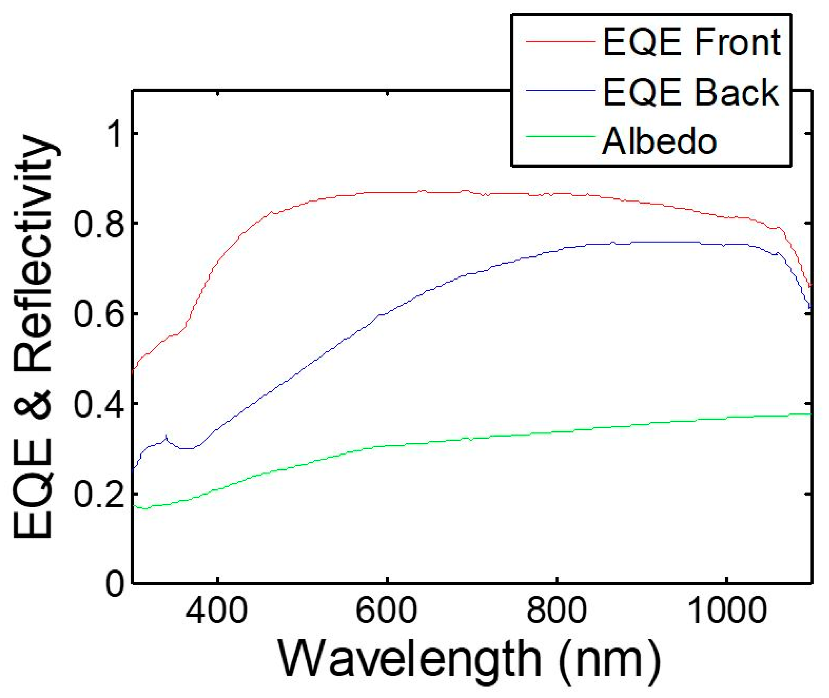
| α | Ground albedo |
| Iback | Incident radiation over the bifacial PV device rear surface |
| Isc,front | Front side component of PV cell short circuit current |
| Isc,back | Back side component of PV cell short circuit current |
| Acell | PV cell area |
| γ | Incidence angle of the solar radiation on the PV module front |
| PV cell semiconductor bandgap wavelength | |
| EQEfront | External Quantum Efficiency for the PV cell front side |
| EQEback | External Quantum Efficiency for the PV cell back side |
| dΩ | Solid angle element |
| shadow | Shadow function |
| As | Ground area |
| Tamb | Ambient temperature |
| Tmodule | PV module temperature |
| NOCT | Nominal Operating Conditions Temperature |
© 2020 by the authors. Licensee MDPI, Basel, Switzerland. This article is an open access article distributed under the terms and conditions of the Creative Commons Attribution (CC BY) license (http://creativecommons.org/licenses/by/4.0/).
Share and Cite
Ricco Galluzzo, F.; Zani, P.E.; Foti, M.; Canino, A.; Gerardi, C.; Lombardo, S. Numerical Modeling of Bifacial PV String Performance: Perimeter Effect and Influence of Uniaxial Solar Trackers. Energies 2020, 13, 869. https://doi.org/10.3390/en13040869
Ricco Galluzzo F, Zani PE, Foti M, Canino A, Gerardi C, Lombardo S. Numerical Modeling of Bifacial PV String Performance: Perimeter Effect and Influence of Uniaxial Solar Trackers. Energies. 2020; 13(4):869. https://doi.org/10.3390/en13040869
Chicago/Turabian StyleRicco Galluzzo, Fabio, Pier Enrico Zani, Marina Foti, Andrea Canino, Cosimo Gerardi, and Salvatore Lombardo. 2020. "Numerical Modeling of Bifacial PV String Performance: Perimeter Effect and Influence of Uniaxial Solar Trackers" Energies 13, no. 4: 869. https://doi.org/10.3390/en13040869