1. Introduction
Patterns of electricity consumption have been receiving great attention in the operation and planning of power systems. Knowing precisely the consumption of electricity reveals energy demand behaviors and enables strategy implementation for increased efficiency and energy intelligence [
1]. These aspects are economically, environmentally, and socially beneficial. Thus, the reduction in payment of electrical bills by consumers, resource-saving by electric companies through delayed grid repowering, reduction of generation costs by reducing the peak demand, implementation of smart microgrids, et cetera, are evidence of economic benefits [
2]. The reduction of electricity demand and/or its peak value leads to decreased
emissions and those of other polluting gases and avoids the construction of new power plants. Moreover, energy efficiency programs benefit society by creating specialized jobs, favoring the economy, the environment and sustainable development.
The energy demand comprises time-series data that are often seasonal and respond to a stochastic process. These data can be classified into four well-known components: irregular, cyclic, seasonal and the trend. The seasonal variations due to temperature, working patterns, and human behavior, cause variations in the energy consumption patterns. These patterns could be used in monitoring systems to detect abnormal consumption [
3,
4]. The detected anomalies can be reported to managers of facilities to take the necessary corrections. However, incorrect patterns could be obtained when the seasonality analysis of electricity demand is neglected [
5].
In recent years, some researchers have studied the electricity patterns for different applications, such as classification, outlier detection, forecasting, energy management, and electricity prices prediction. As will be explained in
Section 2.2, numerous tools and techniques have been used in each methodology. However, the following weaknesses have been detected in our literature review: the seasonality of data is not considered, a detailed information about the electrical consumption profile (ECP) are not taken into account, the structure of time-series data is not analyzed, the selection of training data requires considerable effort, and in other cases, a generalization problem is evidenced because only one case of study was addressed.
In time-series data, there are three types of outliers: the point, collective, and contextual anomalies. As it will be explained further below, few studies have addressed the contextual anomalies detection in the electricity consumption. The contextual anomalies exist when relationships between the different data observations are evidenced. Consequently, finding outliers among data point relationships is a challenge.
In a previous work [
6], the authors presented a novel SAICC (statistical assessment for identifying changes in consumption) methodology to assess the changes in the ECP of buildings. Nonetheless, the effect of time-series treatment in the detection of anomalies was not analyzed. Several methods can be applied for handling the time-series components, including the detrending method [
7] and the seasonal filter [
8]. However, these methods have not produced expected results, which motivated the authors to propose a novel Seasonality Analysis of Electricity Consumption (SAEC) method for times-series treatment.
The results of the above-mentioned time-series treatment methods are compared using the SAICC methodology [
6]. Patterns are obtained in two different scenarios: (i) without performing time-series treatment; and (ii) using three different methods for handling the time-series components, where one method (SAEC) is proposed by the authors in this work. Finally, the ECPs of a year’s real-data are analyzed with each method and their differences in the detection of anomalies are discussed. This method obtains less variable patterns, differentiates between periods of high or low energy demand, and identifies contextual anomalies. Furthermore, it increases the precision and decreases the false positive rate (
) and false negative rate (
) in the anomalies detection of electrical consumption profiles (ECPs). Obtaining less variable patterns and successfull outlier detection could improve electricity management, reduce the time and effort required for data analysis, and improve the performance of energy monitoring systems. Additionally, the conditions that electricity demand data must meet are established, making the times-series analysis useful.
Thus, the main contributions of this work are the following:
The conditions that electricity demand data must meet to make the time-series treatment useful are established.
Detection of abnormal ECPs is improved with the SAEC method, increasing the precision and reducing the and through less variable electrical consumption patterns.
Contextual anomalies in an ECP are identified through the proposed method.
The remaining sections of the paper are organized as follows:
Section 2 provides the background information and related works.
Section 3 describes the SAEC method.
Section 4 details the results, while
Section 5 presents the discussion. Finally,
Section 6 concludes the paper.
2. Background and Related Works
This section presents an overview of the electricity demand as a time-series data, anomaly classification, and hypothesis test applied to outlier detection. Besides, works related to the electricity consumption patterns and detection of anomalies are described.
2.1. Background
The electricity demand is a time-series data that responds to a stochastic process. A time-series data consists of a group of statistical observations recorded over an established period, and it has four well-known components: irregular, cyclic, seasonal and the trend [
7]. It presents fluctuations influenced by various variables, such as ambient temperature, changes in work patterns, and holiday periods. Despite the randomness of these variables, repetitive behaviors (patterns) in the ECP can be identified.
An adequate treatment of time-series components provides useful results regarding pattern recognition. The precision in the detection of anomalies in ECPs is improved, and the and are reduced. Several methods can be applied for handling data series; among the most widespread, are the detrending method and the seasonal filter.
2.1.1. Handling the Time Series Components
Detrending Method
This method subtracts trend line values of the time-series from the original data, thereby obtaining a set of data with zero average. The trend line is obtained based on the least squares method [
9], as follows:
where
t is the time index in the units defined,
is the projected value of the power demand
p [kW] for a value of
t, and
b is the intersection with the axis of the ordinates, that is, the value of
p when
t = 0. Finally,
m is the slope of the line or the average change of
p for each increment of one unit in
t. The least squares method consists of four steps:
Define the variable to analyze; in this case, it is the power demand p, which is variable in time t.
Define a data size n for the analysis, taking into account the sampling frequency with which this data was acquired f.
The sum of the n values of p is calculated.
Calculate the slope
m of the trend line, as well as the intersection with the axis of the variable
p, that is,
b of Equation (1), by means of Equations (2) and (3).
Seasonal Filter
The seasonal filter is a statistical method based on the observation of a data period, where the periodic component of the data is eliminated, resulting in a deseasonalized time-series data. The process is iterative and it can be executed with data from several periods. In this study, data of a full year are analyzed; therefore, the number of periods is 1. The process is detailed below [
8]:
The average power of each week is obtained with the 15-min sampled power data.
The moving average is calculated with terms (where k is the known periodicity of the seasonality); to avoid the loss of information, the first and last value of the obtained moving average is doubled.
An index (multiplicative decomposition) is obtained by dividing the average power of each week obtained in point 1 by the moving average in point 2.
The original 15-min sampled power data is divided for the index obtained in point 3, thereby obtaining deseasonalized time-series data.
2.1.2. Anomaly Classification
An anomaly is defined as a data point that is significantly different from the remaining data set [
10]. Thereby, there are three types of anomalies: point, collective, and contextual. A point anomaly appears when a sampled value shows an unexpected difference from the others. Instead, if data are anomalous in some context but not in another, it is a contextual anomaly. Finally, a collective anomaly contains data that are anomalous compared with the rest of the data instances. In this case, each datum of the group of data could be typical by itself, but their collective occurrence represents an outlier [
11]. In time-series data, outlier detection becomes especially complex when a relationship exists between different data observations (contextual anomaly). In this case, finding outliers among the data points relationships represents a challenging issue [
10].
2.1.3. Hypothesis Testing for Outlier Detection
Hypothesis testing is a procedure that establishes whether the hypothesis is a reasonable statement based on the theory of probability and the statistical evidence of the sample [
7]. The hypothesis is a declaration about a population that must be accepted or rejected after the statistical analysis of the sample. The hypothesis being tested is called the null hypothesis. In this work, the authors define the null hypothesis as the electrical consumption profile (ECP) and is anomalous.
Table 1 defines some terms used later; for example, the false positives (
) are the not anomalous ECP wrongly reported as anomalous.
Evaluation criteria are used to perform comparisons in hypothesis testing, such as
,
, precision, sensibility, and specificity. The
and
are defined as follows:
The precision is defined as the percentage of reported anomalous values that truly are anomalous. On the other hand, the sensibility or recall represents the percentage of true anomalies reported as anomalous. Finally, the specificity is the ratio between the number of PCE reported as not anomalous, and the total truly negatives [
10]. These criteria are defined as follows:
2.2. Related Works
In recent years, some researchers have studied the electricity consumption patterns, where five main application areas can be identified: (i) forecasting; (ii) energy and load management; (iii) electricity prices prediction; (iv) classification; and (v) outlier detection. The different proposed works are used for electricity and economic sector planning, customer classification, tariff establishment, energy efficiency programs, cost reduction, detection of fraud, anomalies, failures, et cetera. For this, numerous tools and techniques have been used in each methodology; however, five types of weaknesses have been detected:
- (a)
The seasonality of data was not considered.
- (b)
A detailed information about the electrical consumption profile (ECP) was not taken into account.
- (c)
The structure of time-series data was not analyzed, therefore the methodology can be improved.
- (d)
The selection of training data requires considerable effort.
- (e)
Generalization problem is evidenced because only one case of study was addressed.
Over time, scholars have developed new proposals for forecasting electricity demand [
12,
13,
14,
15]. Actually, artificial intelligence (AI) techniques are preferred over others. However, some difficulties are evidenced in these types of methods; in particular, the previously identified weaknesses type a, b, d, and e. For instance, the effect of seasonality in the training phase of these methods is difficult to establish, and generally, the selection of training data needs considerable effort, often requiring the prediction of input variables, which induces high uncertainty. Moreover, the application of AI methods does not guarantee it can be used for other cases, deriving in generalization issues like in [
14]. The reviewed works about the application area of energy and load management evidence weakness type a and b. In some cases, like in [
16,
17], the seasonality is not addressed, and detailed information about the ECP is neglected, reducing the capacity of the method to work in real-time. The electricity demand behavior also has been used for price prediction by some authors like Cuaresma et al. [
18] and Janczura et al., [
19]. Although they consider, to some degree, the effect of seasonality, an in-depth examination using an adequate approach could yield better results. For example, detailed information about ECPs is ignored, and on the other hand, the used models fit specific data cases; therefore, their application to other cases can be unreliable.
The most representative studies about the classification of ECP and outliers detection evidence weakness type a, b, c or d. This is because various clustering techniques ignore the time-series context of data, and consequently the seasonality effect is missing as in [
20,
21,
22]. Some authors like Seem [
23,
24] and Li et al., [
25] use only the mean daily-energy and the peak daily consumption in pattern recognition, hence, it is diffiicult to perform a detailed analysis of the ECP. On the other hand, Capazzoli et al. [
26] characterize the energy time series in time windows, which impede real-time (or near real-time) analysis. Meanwhile, other studies apply machine learning to detect outliers in electricity consumption, for instance, Jokar et al., [
27] use support vector machines and unsupervised learning (k-means), while Fenza and Gallo [
28] apply LSTM neural networks and statistics. In both cases, the selection of training data requires considerable effort, and the time-series analysis was not considered.
Recently, the identification of contextual anomalies has been discussed as a new challenge in electricity monitoring. For this purpose, scarce studies have addressed the topic. In particular, Araya et al. [
29] propose an ensemble anomaly detection framework with several outlier detection classifiers using majority voting. Similarly, Hayes and Capretz [
30] propose a contextual anomaly detection framework also using majority voting. These proposals do not analyze the structure of time-series data and require high computational expense; thus, evidencing the identified weaknesses type c and d. In addition, only values less than zero were considered noisy in data pre-processing. Alternatively, Cui and Wang [
31] propose an anomaly detection system based on a polynomial regression model and Gaussian distribution. Although this study obtained an
equal to zero in all analyzed cases, only an upper threshold is used to identify contextual anomalies, hence outliers of low consumption cannot be reported.
Besides, Fan et al. [
32] investigate different autoencoder architectures and training schemes in detecting anomalies in building energy data. This study works in a high-dimensional and large-scale data scenario since it states that statistical methods are not scalable and adequate. Nevertheless, this methodology requires considerable high computational effort in each stage; for instance, to establish the most influential variables in energy consumption (Month, Day Type, and Hour) and the most dominant period (24 h), which usually is well-known. Additionally, various masking noise levels are used to produce corrupted subsequences to enable autoencoders to learn better. This study contributes interestingly to the field of knowledge. However, in the opinion of the authors, in most cases, it is unnecessary to address the anomaly detection of electricity demand in the big data field.
Table 2 summarizes the shortcomings found in the application of electricity patterns. In this context, the authors have proposed a specific method to obtain patterns and detect anomalies in the electricity demand.
3. SAEC Methodology and Seasonality Analysis
Based on the limitations detected in
Section 2.2, the authors propose a simple method to address the weaknesses detected to improve patterns obtention and anomalies detection in electricity consumption. The proposed SAEC method is able to: (i) address time-series structure appropriately through a robust methodology; (ii) use a resolution of 15 min sample data to allow near real-time outlier detection; (iii) be used for analyzing any type of electrical consumption; (iv) increase the precision and reduce the
and
in the detection of anomalies; and (vi) identify contextual anomalies in electricity demand.
3.1. Confirmation of Seasonal Variation in the Electrical Consumption
The application of SAEC method guarantees better performance when series data shows seasonal variation. The authors recommend handling the time-series components of electricity consumption when the following conditions are met:
Fluctuations have a defined pattern
Fluctuations have defined periods
The values of the time series follow a linear trend
The amplitude values in each period are similar in each cycle.
To verify compliance with the above conditions, the electricity consumption data of two different facilities are analyzed. The first installation is the 5E building of the Universitat Politècnica de València (UPV) in Spain, whose data was obtained through the Derd System [
41]. The second installation corresponds to the power supply connection of the Universidad Politécnica Salesiana (UPS) in Cuenca, Ecuador. The two facilities are located in different countries, so the users’ energy consumption behaviors differ significantly.
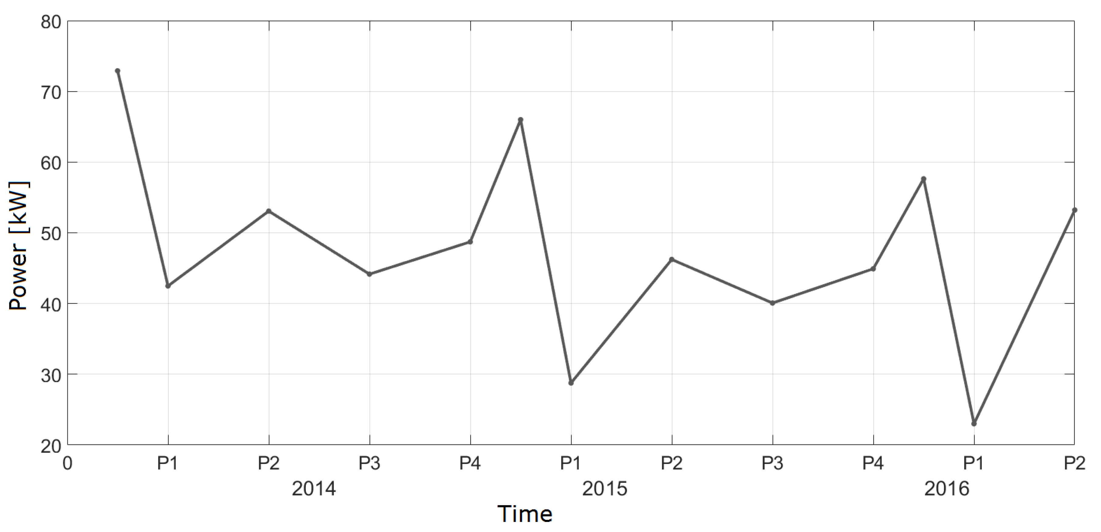
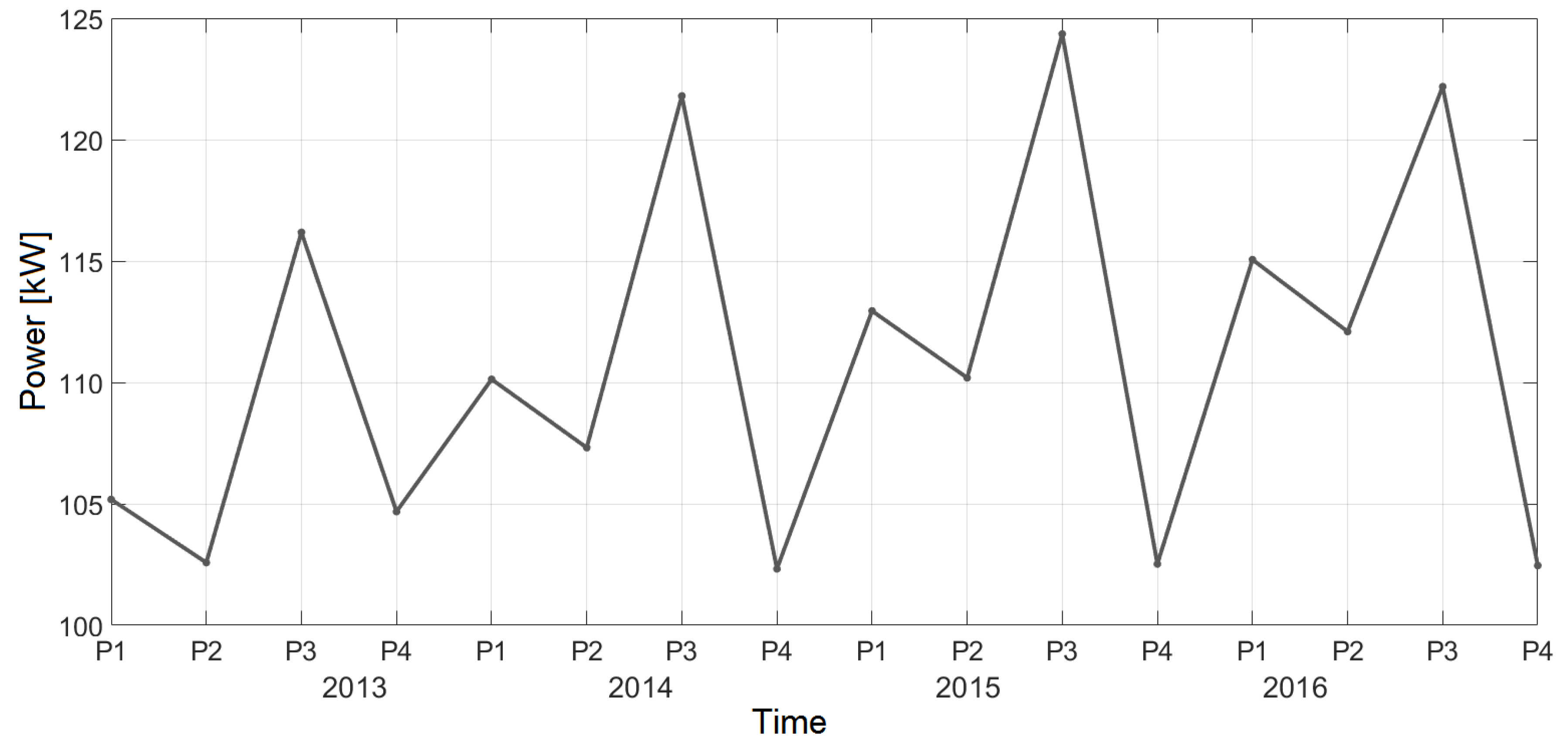
Figure 1 and
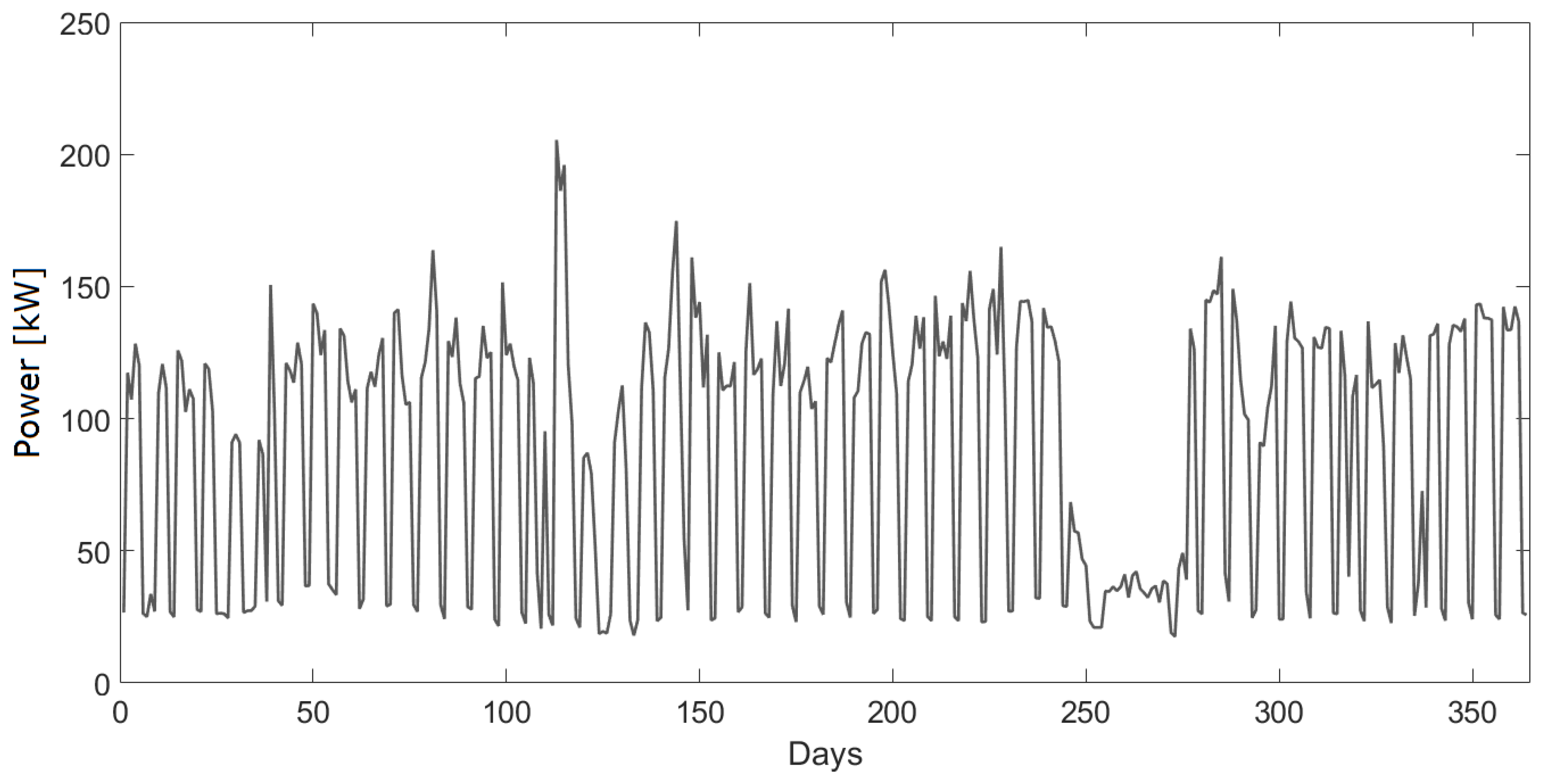
Figure 2 show the quarterly average power consumption for each installation. The fluctuations defined in periods of one year are clearly visible. Moreover, in the UPV case, the data follow a negative linear trend, while in the UPS case, the linear trend is positive. The amplitude of the values in each period of every cycle is similar: increasing and decreasing as per the linear trend. Thus, the four mentioned conditions are satisfactorily fulfilled, so handling time-series components can be carried out in both cases. Observing the scale of the figures shows that the seasonal component of UPS electricity consumption is weaker than UPV consumption.
The authors propose a new SAEC method, specially designed for electricity demand data, which eliminates the trend and seasonality of the time series data. This method has the advantage that it can be applied when just one-year data is available. It is important because the electrical consumption patterns change over time.
3.2. Seasonality Analysis for Electricity Consumption Method (SAEC)
The proposed SAEC method provides better-defined patterns while maintaining the same level of confidence. The first consideration is that seasonality has a marginal influence on the base load value of consumption because, in “non-working hours,” there is no occupation for which the electricity demand remains practically constant. The proposed method is thus detailed below:
A vector of the 15-min sampled power data only for the working days is obtained for the analyzed period, and the amount of working days that make up each week is recorded.
The base load value is calculated, for which the first percentile of the vector of the 15-min sampled power data in point 1 is computed. Analyzing the vector shows that the quantity of the anomalous low value is less than 1% of the data. Therefore, measurements corresponding to events such as power outages, disconnections, and measurement errors are ignored.
The base load value is subtracted from the vector of the 15-min sampled power data in point 1. Hence, the resulting vector has values close to zero during the non-working hours. This is useful for the analysis because the seasonality of consumption has minimal influence during these hours.
The average power of each week is obtained by considering only the number of working days recorded in point 1.
The moving average of the values obtained in the previous point is calculated; four values are used, corresponding to four weeks.
The centered moving average is calculated by averaging the two consecutive values obtained in point 5.
The average of all values obtained in point 6 is calculated.
The seasonality index for each week is obtained by dividing each value obtained in point 6 by the value obtained in point 7. Thus, the average of the seasonality indexes is 1.
The vector obtained in point 1 is detrended and deseasonalized at the same time, by dividing each of its values by the corresponding seasonality index for each week (point 8).
The base load value is added to each datum of the deseasonalized vector of the previous point.
The data vector of electricity consumption is reconstructed by combining the correct sequence of the deseasonalized working days and the non-working days data that were initially separated.
Once the SAEC method is applied, the results become apparent.
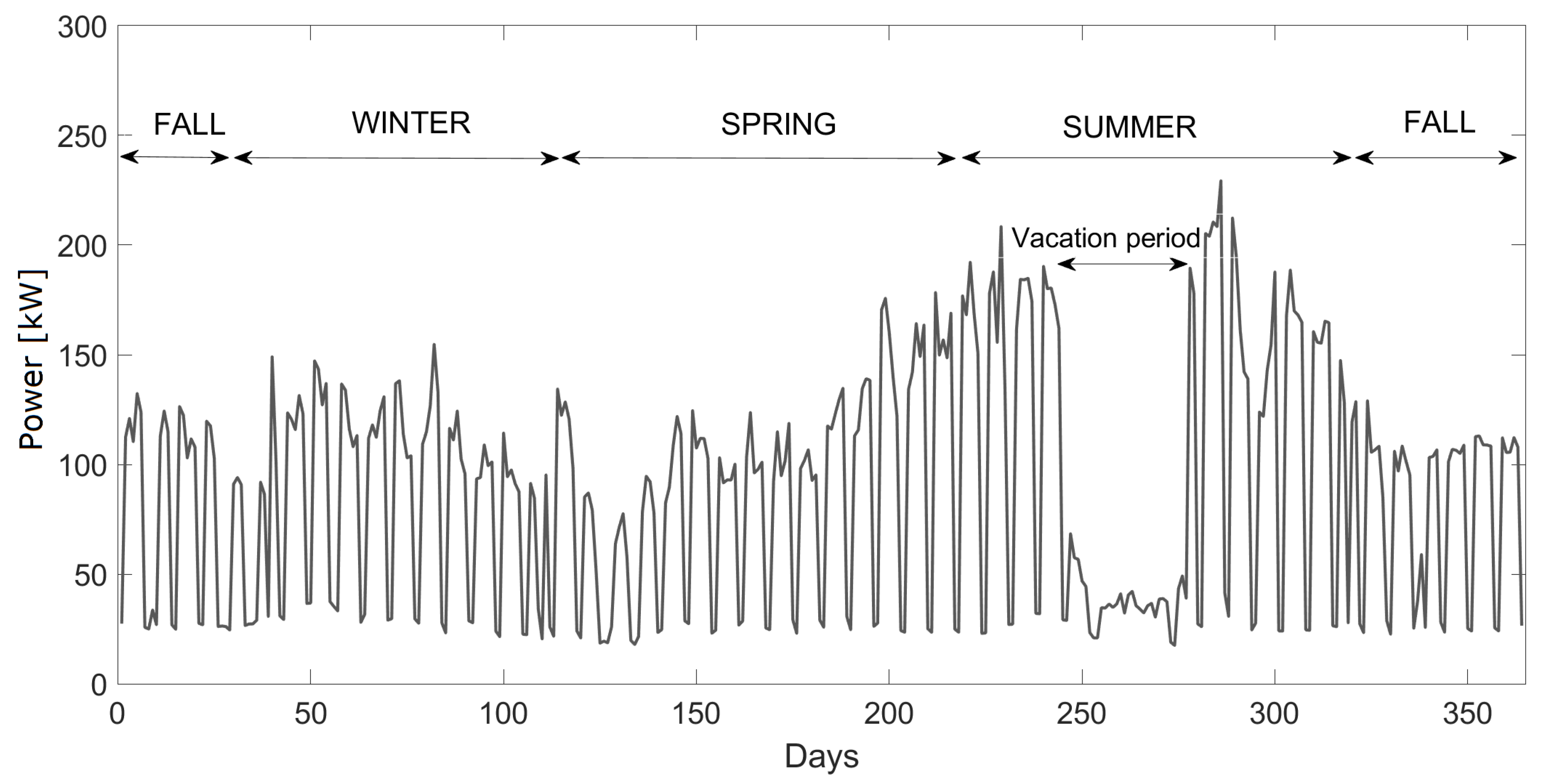
Figure 3 shows the one-year electricity consumption of the 5E building of UPV (average power of the highest 15-min sample data for each day). Observe that the electricity consumption presents significant fluctuations in the different seasons, which is typical for the Spain’s buildings, as in other countries with pronounced seasons. The obtained detrended and deseasonalized data is depicted in
Figure 4.
Similarly,
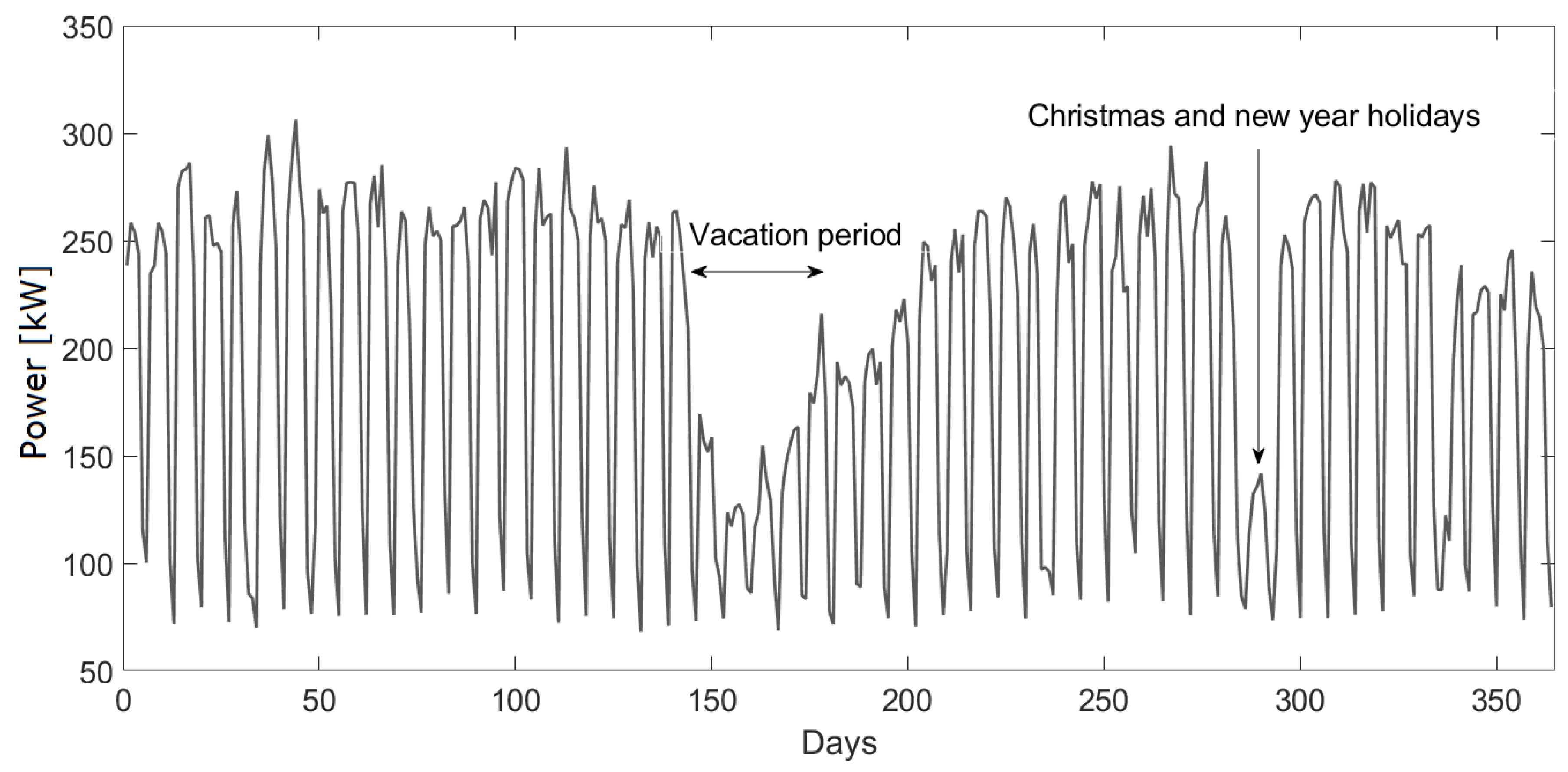
Figure 5 shows the one-year power consumption of UPS (average power of the highest 15-min sample data for each day), and
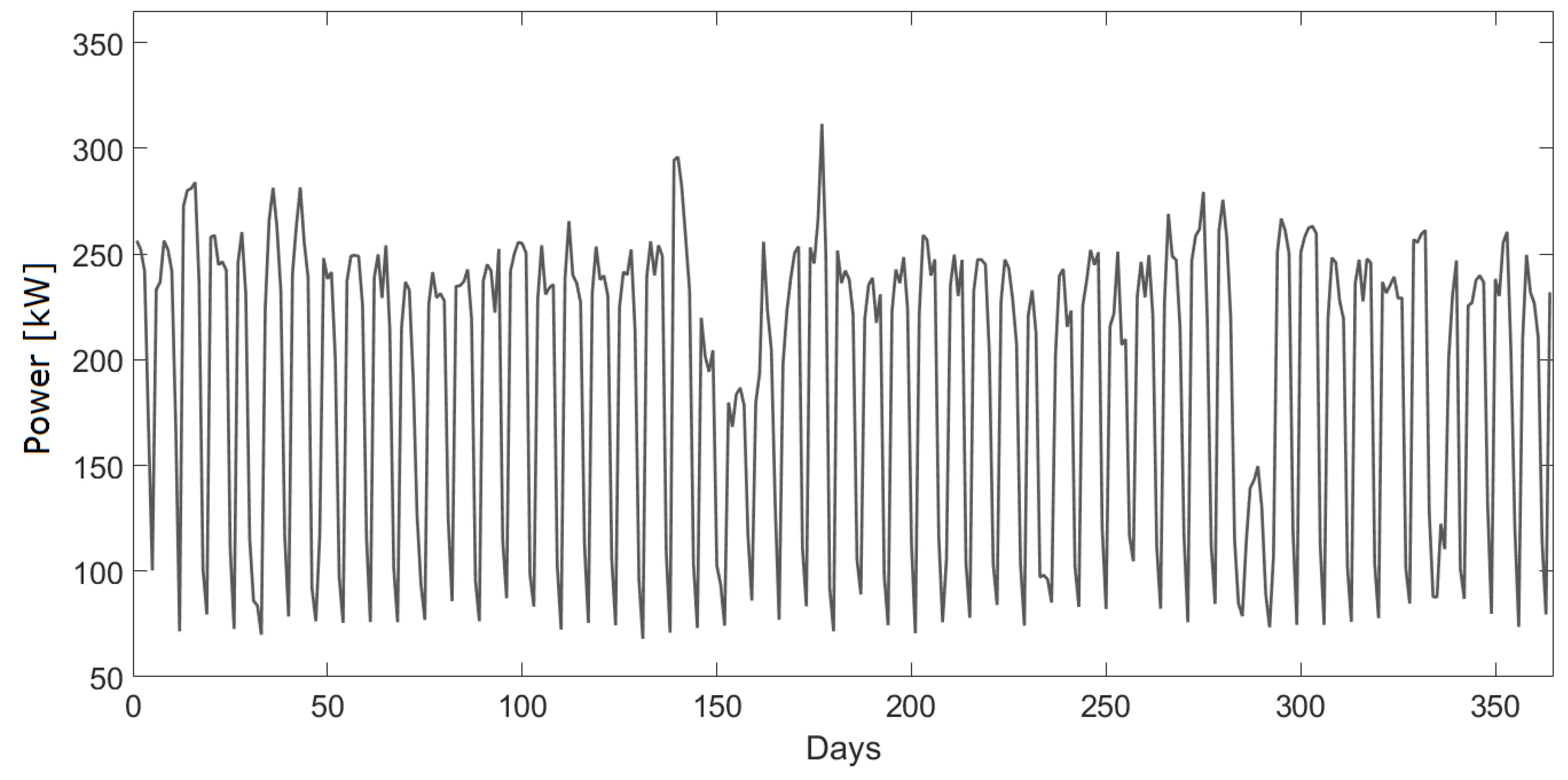
Figure 6 shows the deseasonalized electricity consumption. The SAEC method transforms the initial data into a stationary time series. To avoid losing information that is required later, the seasonal indexes of each week are stored. In this case, no electricity consumption fluctuations are corresponding to seasons because seasonal temperature fluctuations are small in Ecuador. The fluctuations correspond to power decreases in vacations, Christmas, and New Year holidays.
The performance of the SAEC method is compared with two existing methods for handling data series, which are the detrending method and the application of a seasonal filter.
3.3. Application of Deseasonalization Methods
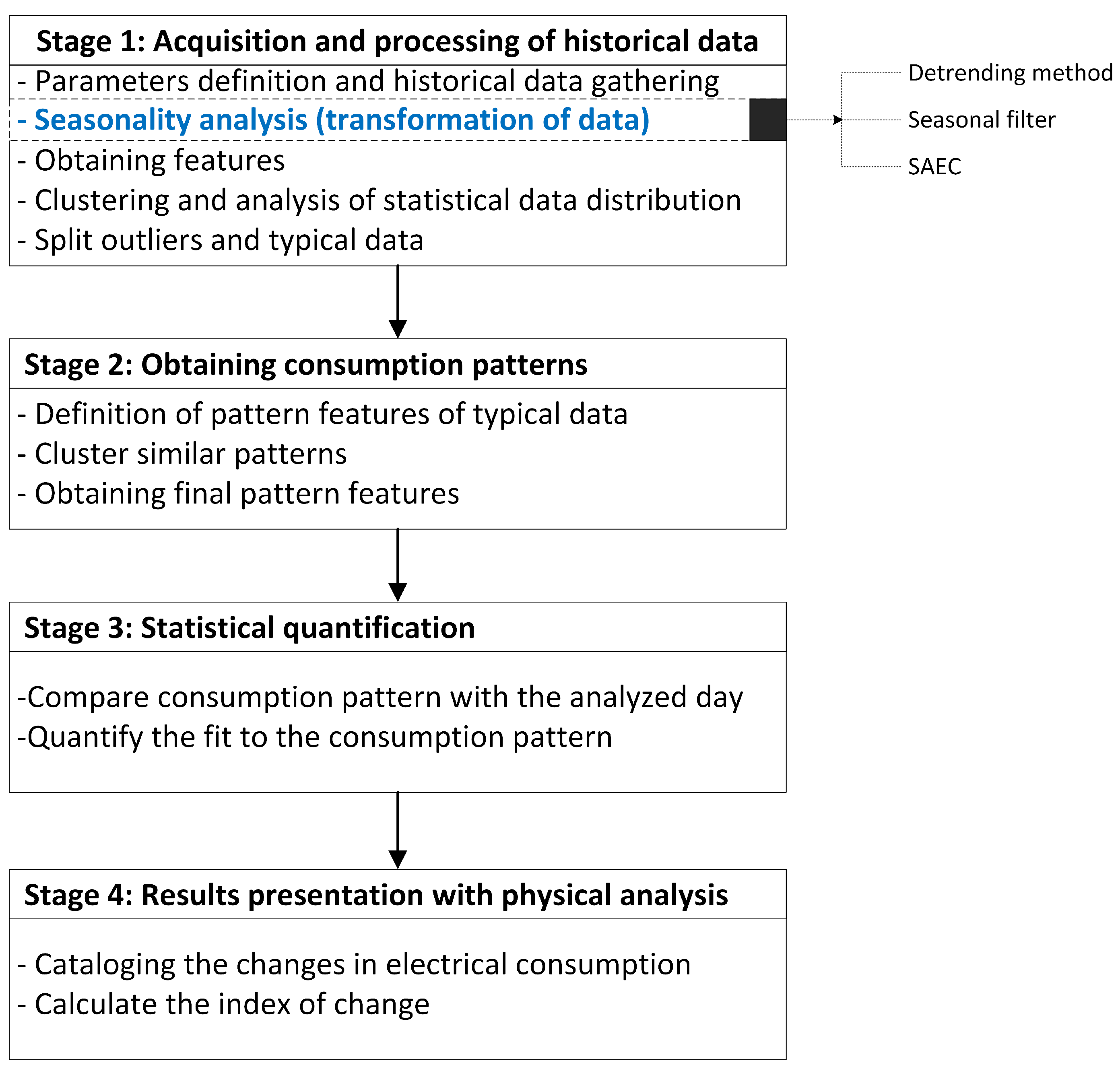
The SAICC methodology was first developed by the authors in a previous study. It finds patterns and statistically quantifies the changes in an ECP [
6]. This methodology establishes conclusions that give clues about the possible causes of changes in electricity consumption. It also presents an index of change that quantifies and catalogs the anomalies in ECP.
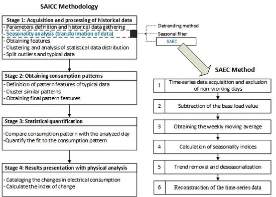
The SAICC methodology consists of four stages: (1) acquisition and processing of historical data; (2) obtention of consumption patterns; (3) statistical quantification; and (4) presentation of results [
6].
Figure 7 shows a simplified block diagram of the SAICC methodology, where the transformation of time-series data is carried out through three different methods: detrending method, seasonal filter, and SAEC. The first two methods are the most commonly used in temporal series, while the third method is proposed by the authors. This is done in order to compare results using these different techniques.
4. Results
The objective of this work is to evaluate the time-series treatment in obtaining patterns and detecting anomalies in ECPs. This study compares the patterns and anomalies detected using different analysis methods for handling time series components:
Without seasonality analysis (WSA)
Detrending method (DM)
Seasonal filter (SF)
Seasonality analysis for electricity or energy consumption (SAEC), proposed in this work.
As mentioned above the electricity consumption of two different facilities is analyzed in this work. The first one is the 5E building of the UPV in Valencia, Spain, whose data were obtained through the Derd system [
41] from 28 November 2015 to 27 November 2016. The second facility is the UPS in Cuenca, Ecuador, with data from 9 March 2017 to 8 March 2018. These two case studies are interesting because they are in distant countries and their consumption patterns differ significantly.
4.1. Obtained Patterns
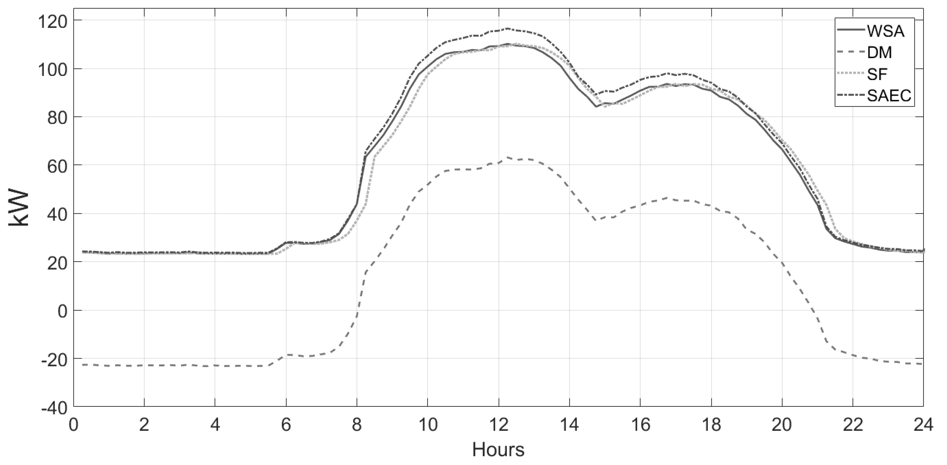
The authors now present the differences between the patterns obtained for each seasonality analysis method, and interpretation thereof, according to the SAICC methodology. The case of a working Wednesday in the 5E building of UPV is presented.
Figure 8 shows the mean pattern obtained for each method used. The mean pattern obtained with the WSA method is similar to that obtained by the seasonal filter and SAEC methods. In working hours, the pattern obtained by the SAEC method has values slightly higher compared with others. On the other hand, an offset presents itself in the pattern obtained by the detrending method.
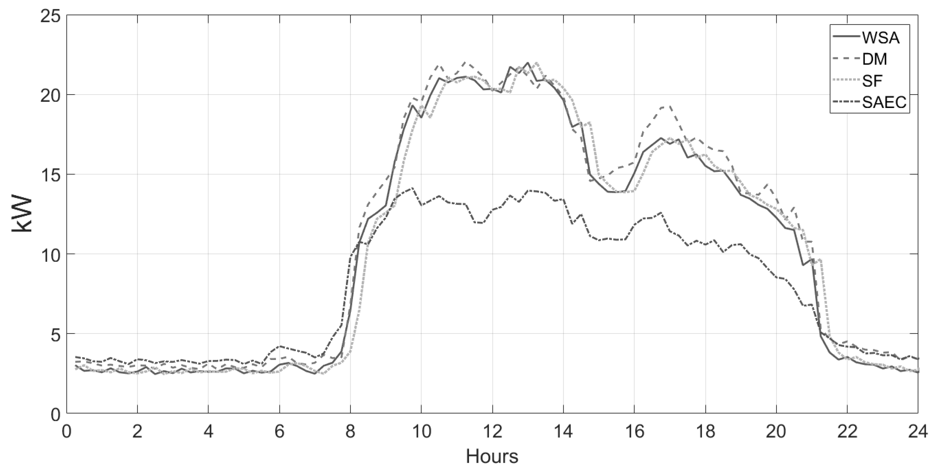
Figure 9 depicts the standard deviation values. No significant variations are observed when applying the WSA, detrending method, and seasonal filter. On the other hand, when the SAEC method is used, the standard deviation decreases considerably in working hours. This is relevant because it indicates that the pattern obtained with this method is less variable, and therefore more defined. This effect is a major advantage because, when detecting abnormal ECPs, the precision increases, while the
and
decrease evidently (see
Section 4.2).
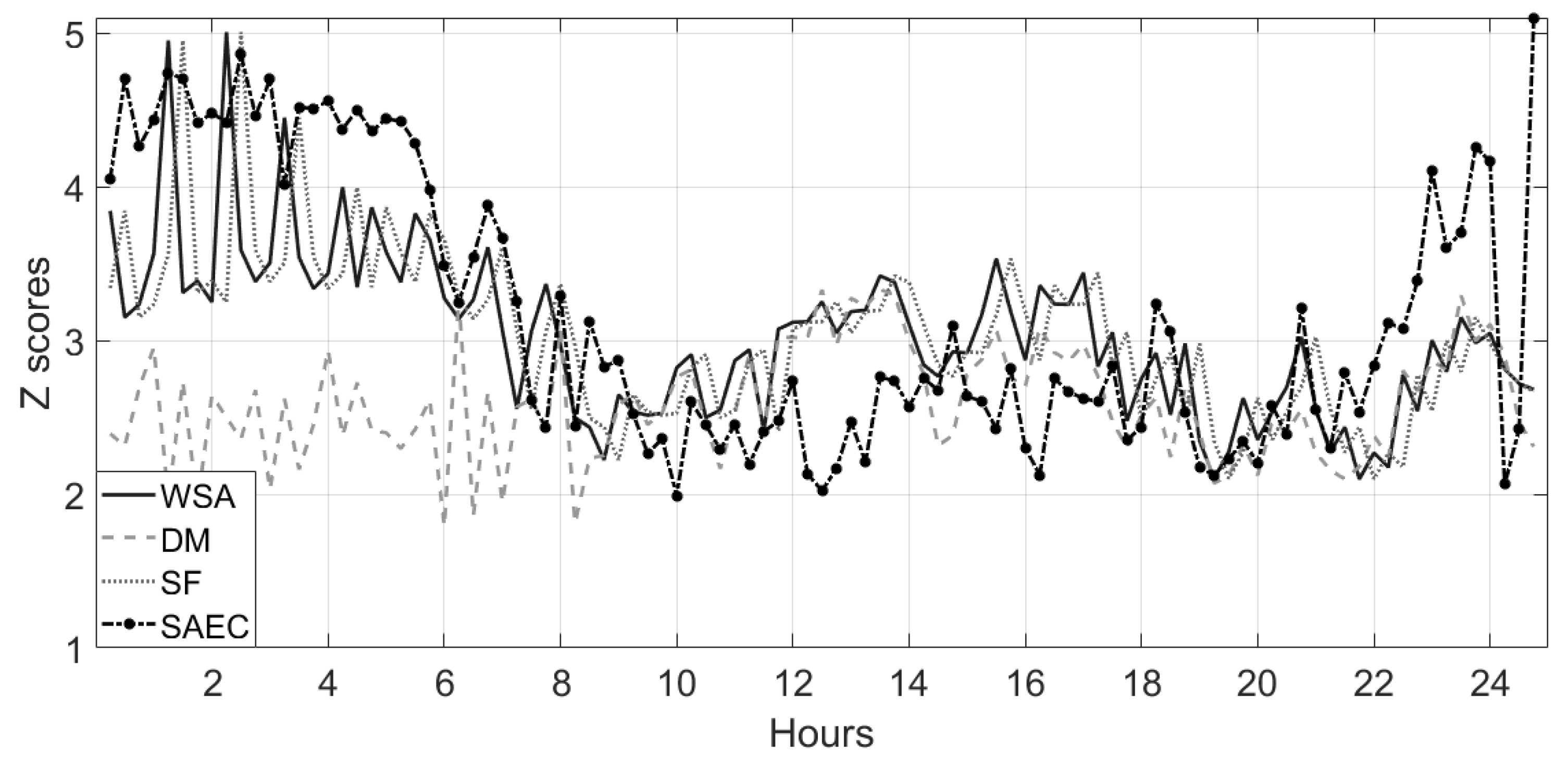
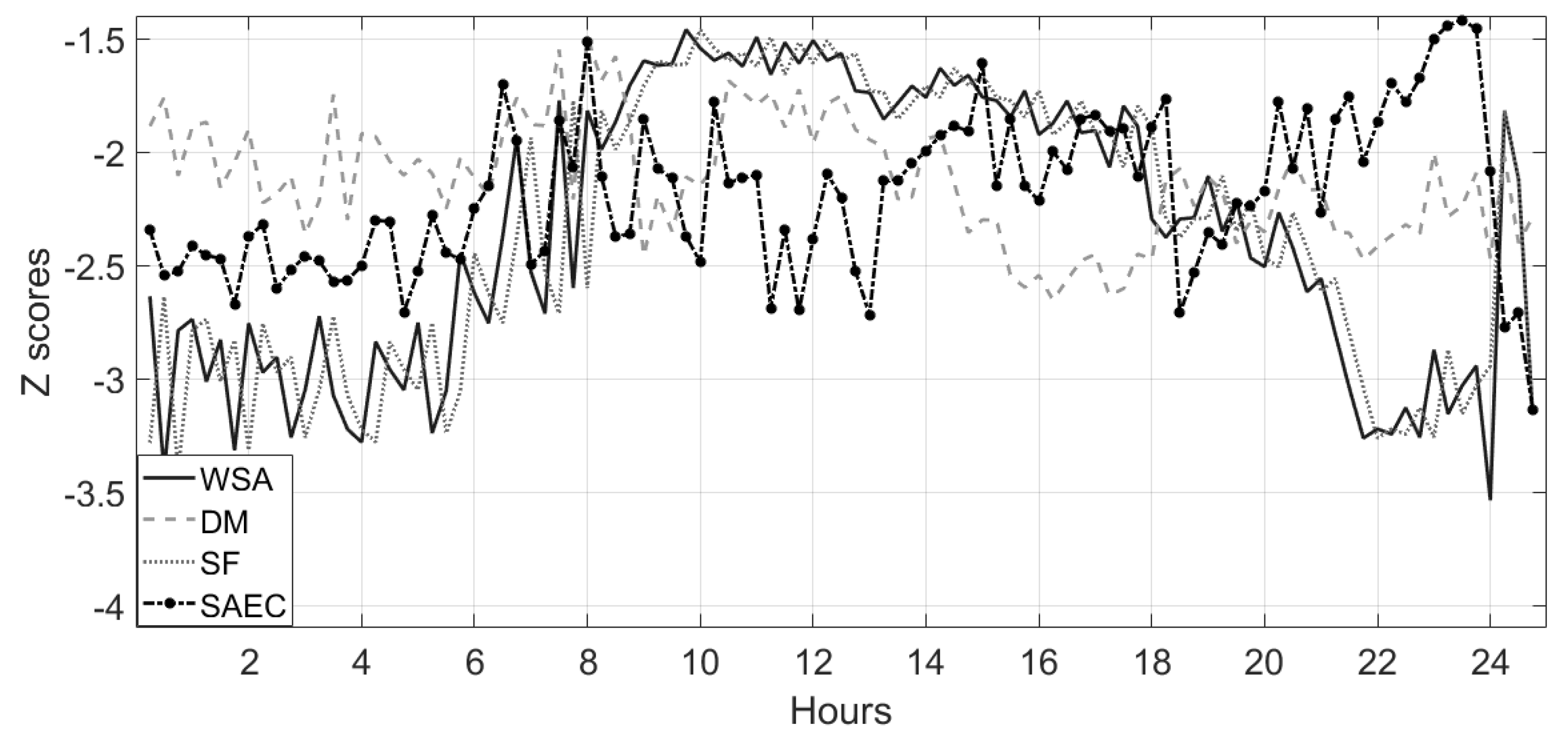
In
Figure 10 and
Figure 11, the
and
values obtained represent the upper and lower limits of each confidence interval of the consumption pattern (a value is considered anomalous when it is outside this interval). The results from the seasonal filter are very similar to those obtained using the WSA method. The detrending method obtains smaller confidence intervals in the non-working hours because of its limited capacity for grouping days with similar consumption. The proposed SAEC method, in some cases, obtains larger confidence intervals, but smaller ones in other cases. Therefore, the values of
and
alone do not indicate whether one method is better than the other. Hence, the
is a key indicator in this analysis.
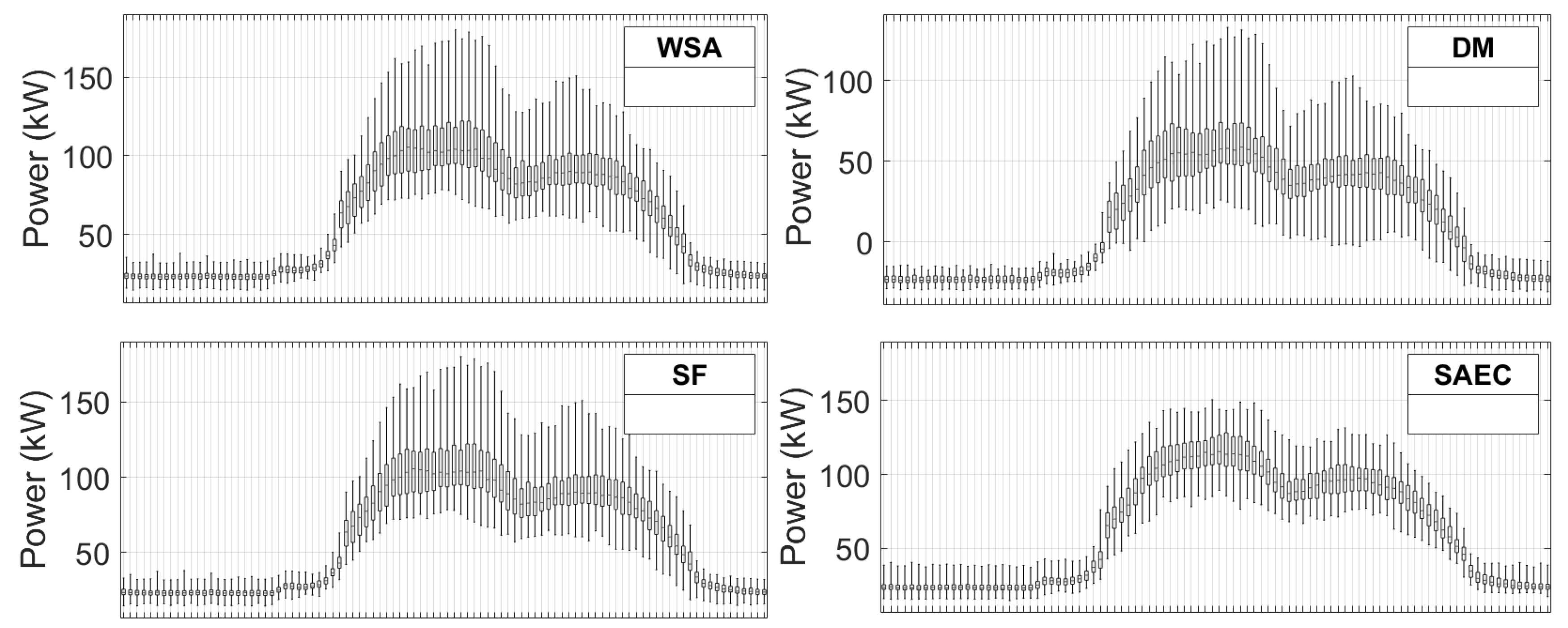
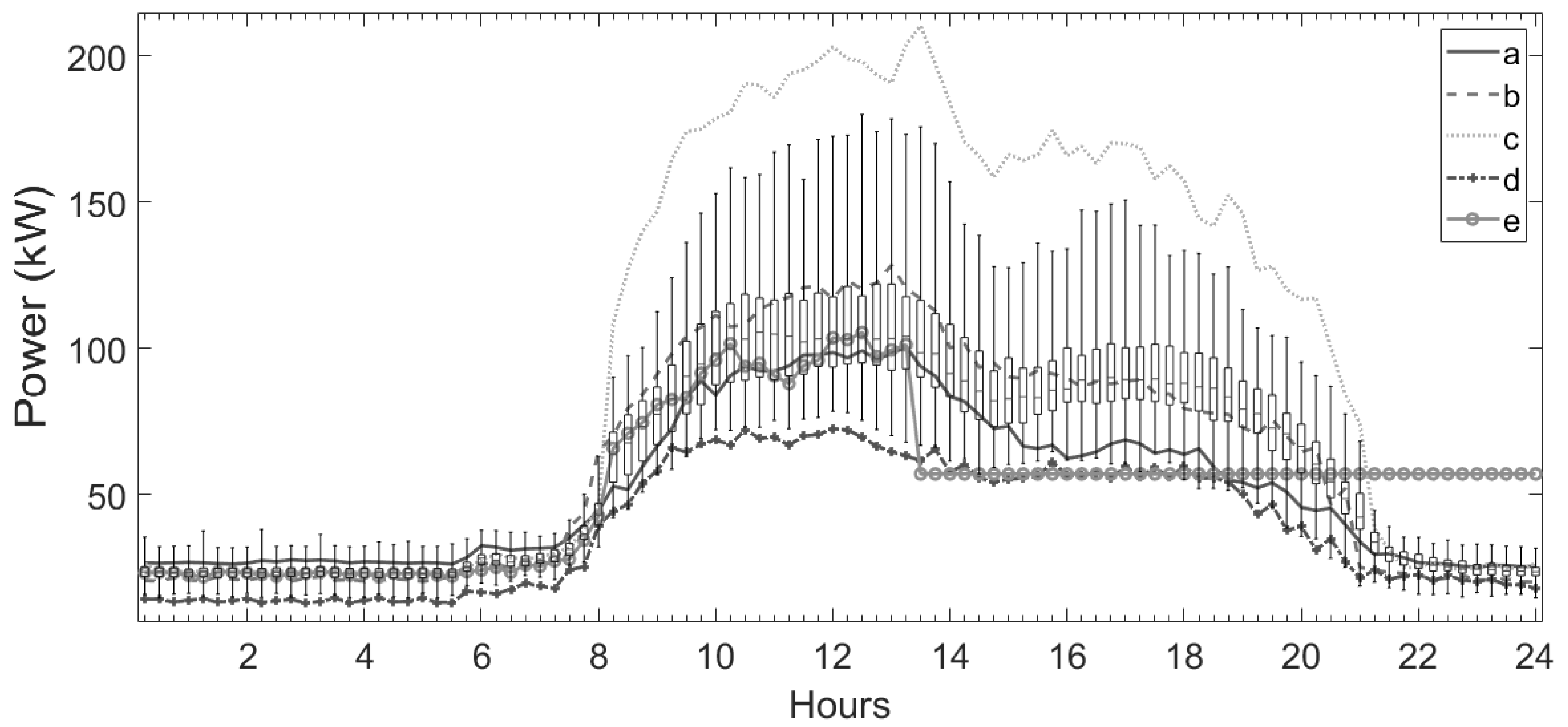
The patterns obtained with one-year data can be represented by box-plots (see
Figure 12). Evidently, the detrending method and seasonal filter do not produce a very different pattern from that produced by the WSA method. The SAEC method obtains a less variable pattern while maintaining the same level of confidence. That is, electricity consumption is better defined, and hence the detection of changes and anomalies is more reliable. This pattern represents the typical electricity consumption on a specific day of the week and can be assigned to any week of the analyzed period through the seasonal indexes explained in
Section 3.2. The success of the method lies in improving the
, even when the consumption pattern has less variation.
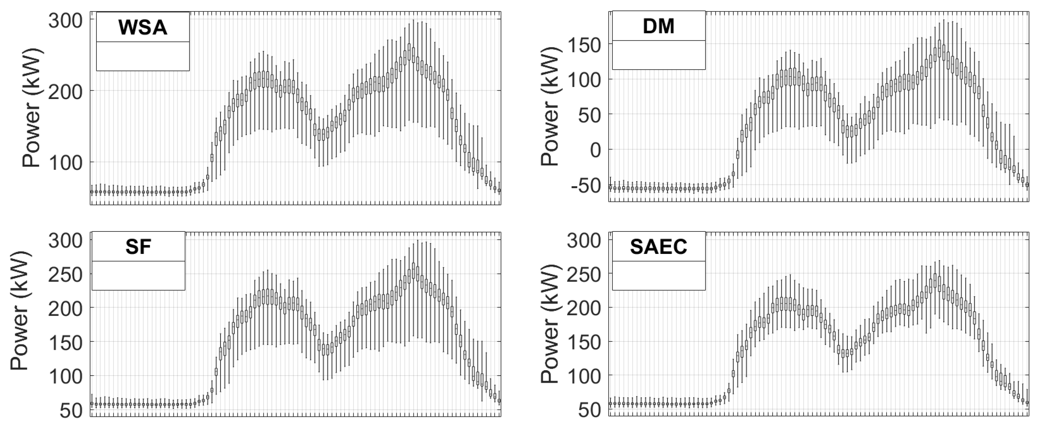
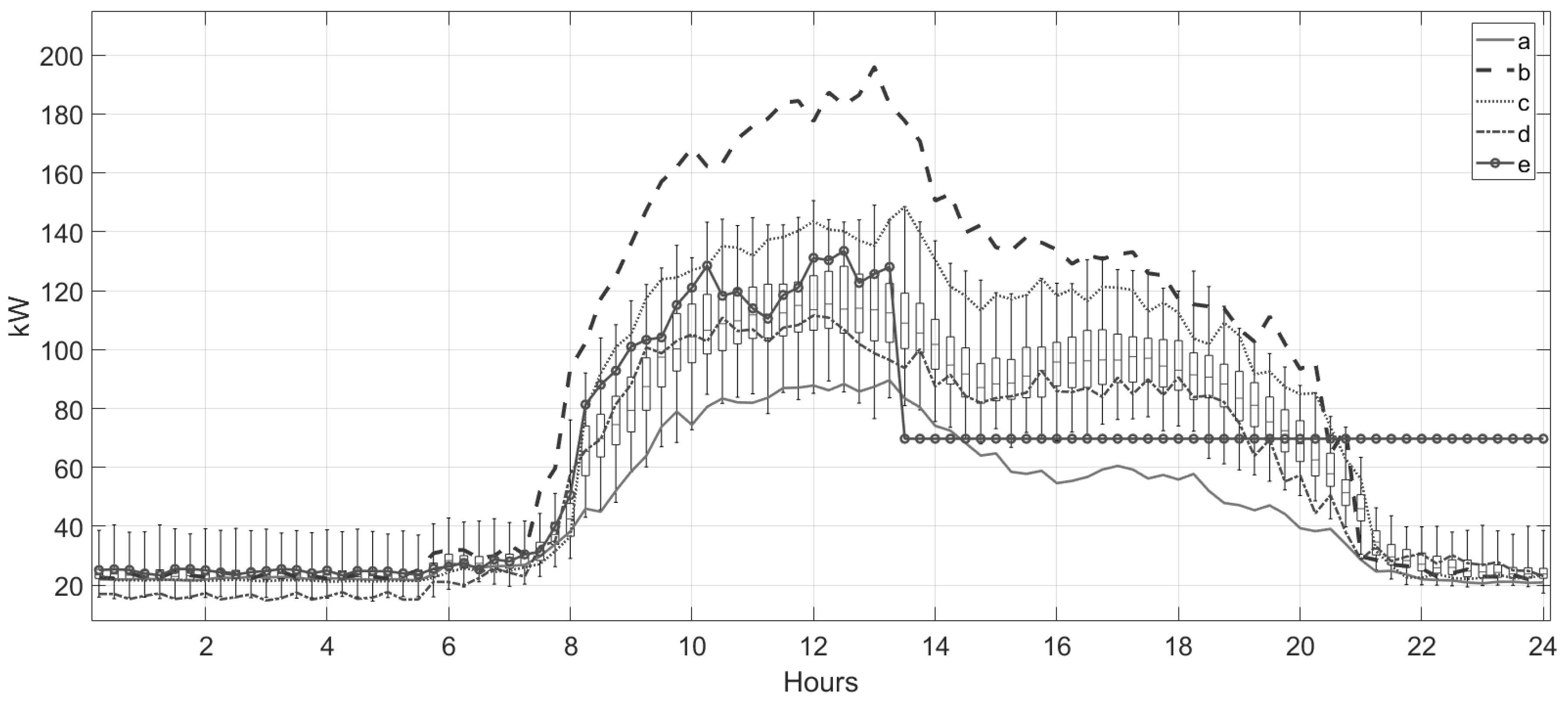
The conditions to carry out the time-series treatment of electricity demand were established in
Section 3.1. The annual electricity consumption of UPS satisfies those conditions. However, the seasonal component is small because of the nonexistence of the four climatic seasons in areas near the equator. Applying the SAEC method shows that the pattern obtained is less variable than the patterns obtained by the other methods (see
Figure 13). This result indicates that, although the seasonal component is small, an adequate time-series analysis obtains a less variable consumption pattern. This suggests that the method can be used for any type of electrical consumer.
4.2. Anomaly Detection
Once the consumption patterns have been defined, the corresponding statistical analysis is carried out to detect anomalies in each day of the week.
Table 3 details the obtained patterns for different working Wednesdays and Fridays in the 5E building of UPV. The details include: number of ECP reported as typical, number of ECP reported as anomalous, number of truly anomalous ECP (identified by an expert human), the anomalous ECP reported as anomalous (
), the anomalous ECP reported as not anomalous (
), the
, the
, and the precision.
A time-series treatment through the SAEC method can identify as typical (
) to ECPs affected by seasonality whose power consumption is distant from the mean in each 15-min interval, which would have been labeled as anomalous (
). This is because there are weeks with normally high electricity consumption and weeks where consumption is normally low. The SAEC method allows such ECPs to be labelled as non-anomalous, thus reducing the
. This can be seen in the case of Wednesday and Fridays in
Table 3.
In comparison with other methods, the SAEC method easily reports abnormal ECP when consumption is high, but it is produced in weeks where consumption is usually low or vice versa (
).
Table 3 shows the pattern of a working Friday. Here, in the time-series treatment with the SAEC method, fewer ECPs are considered typical, which helps obtain a pattern with smaller confidence intervals. Thus, the number of anomalous ECPs detected by the SAEC method increases, which negatively affects the
. However, the
decrease from 47.1% to 11.8% and the precision increases from 69.2% to 71.4%. Besides, the application of the SAEC method allowed the expert human to catalogue as unusual the consumption of four additional Fridays that he had not previously perceived.
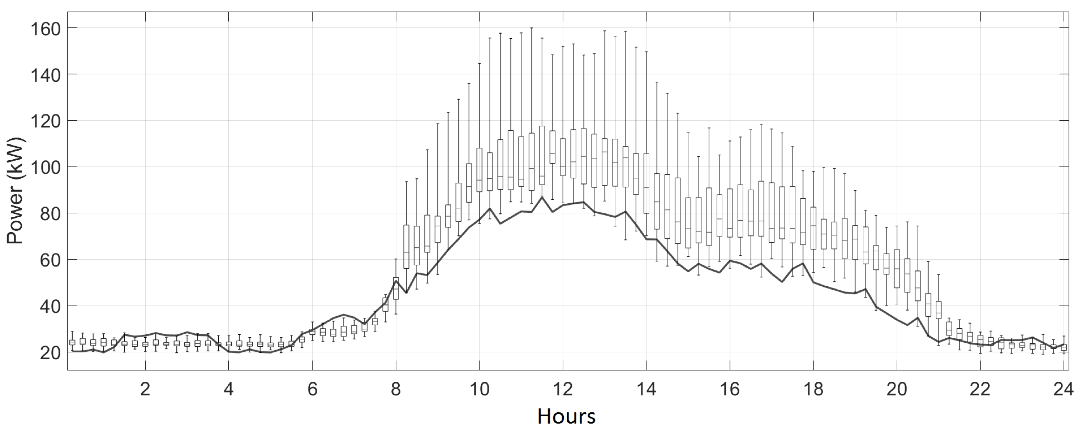
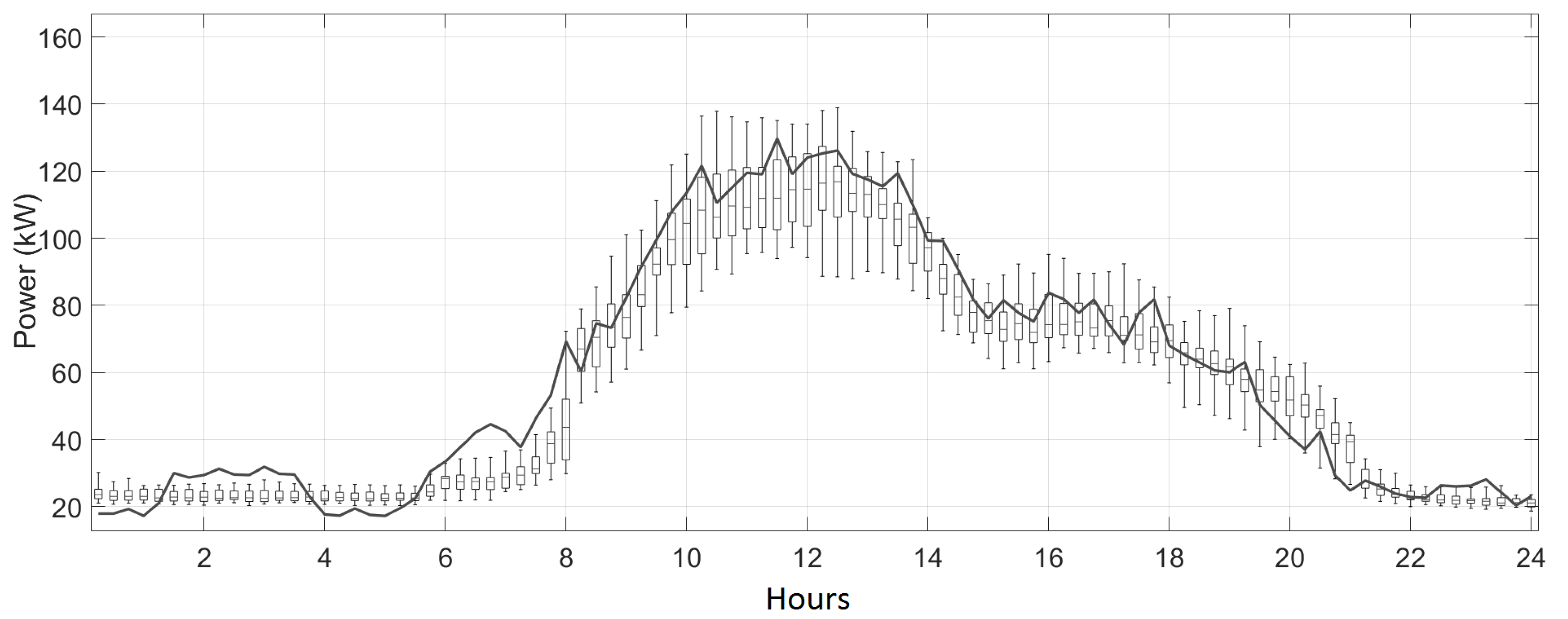
Figure 14 and
Figure 15 show one of the four abnormal Fridays detected by the SAEC method and its corresponding pattern with the SF and SAEC methods, respectively. In the first case, the human expert indicated that electricity consumption on that day was not anomalous because the energy requirement was low during that period of the year. However, when comparing the analyzed day with the pattern obtained with the SAEC method, an anomalous consumption is perceived between 1:30 a.m. and 3:30 a.m. and between 6:00 a.m. and 7:15 a.m., a critical issue not noticed before. The comparison was made only between the SF and SAEC methods because the patterns obtained with the DM method and WSA are similar to those obtained by the SF one.
Table 4 shows the details of the detected anomalies for different working Wednesdays and Fridays in the power supply connection of UPS. The time-series treatment of electricity demand of UPS with the SAEC method reduces the number of
(Truly anomalous PCE reported as typical) for Wednesdays, as shown in
Table 4. In this context, the SAEC method can identify weeks of usually low consumption, improving the precision of the anomalies detection. On the other hand, the
does not always improve, as in the case of Fridays. However, in this same case, the
and the precision improve considerably.
5. Discussion
The results obtained suggest that the use of the SAEC method improves the detection of abnormal PCE by differentiating between periods of high or low energy demand, thus identifying contextual anomalies, which are difficult to detect. The method guarantees a significant improvement in the precision of anomaly detection when electricity demand meets the four conditions for carrying out the time-series treatment (defined in
Section 3.1).
A pattern with large confidence intervals does not easily detect abnormal ECPs, whereas a pattern with small confidence intervals labels too many ECPs as anomalous, which is not convenient. The proposed methodology significantly improves the identification of consumption patterns and the detection of anomalous data.
Table 5 shows the adjustment of six ECPs through the four different methods referred above. In the first four selected ECP, the SAEC method outperforms the others by avoiding the
and
in periods where the energy demand is usually high or low. However, it obtains the same results as the other methods when there are measurement errors or when the ECP has an unusual shape.
Figure 16 and
Figure 17 show the difference between the SF and SAEC methods for the detection of anomalies for five abnormal Wednesdays (first five ECPs of
Table 5). The consumption patterns, which are obtained by the DM method and WSA are similar to those obtained with the SF. Thus, only the comparison between the SF and SAEC methods is presented.
The errors reduction in the identification of changes and/or detection of anomalies in electricity consumption allows efficient energy management, reduce costs and electricity consumption, detect abnormal consumption and failures, and save time for technicians and managers in charge of a building’s facilities. It also provides more reliability for surveillance operations in preventive and operational systems. The proposed system is hence advantageous without high computational expense in comparison with other methods.
Finally, we emphasize that the influence of the time-series treatment in obtaining patterns and detecting outliers in electricity demand is significant, thus, it deserves special attention. The results suggest that with the application of the SAEC method, contextual anomalies can be identified, additionally to the point and collective anomalies. This is because the method recognizes periods of usually high or low energy consumption. Besides, the precision in anomalies detection increases; in cases where the increases, it does it slightly, while the decreases substantially. On the other hand, when the increases, it does it slightly while the decreases substantially. The results also suggest that the method can be used for diverse types of electrical consumers, in which the seasonal components of the time series have a different structure.
6. Conclusions
In a previous work, the authors of this work presented a novel SAICC (statistical assessment for identifying changes in consumption) methodology to assess the changes in the ECP of buildings. Nonetheless, the effect of time-series treatment in the detection of anomalies was not analyzed. Several methods can be applied for handling the time-series components, including the detrending method and the seasonal filter. However, these methods have not produced expected results, which motivated the authors to propose a novel Seasonality Analysis of Electricity Consumption (SAEC) method for times-series treatment.
The novel SAEC method significantly improves the capability of obtaining electrical consumption patterns without the use of additional methods that require more time and computational effort. In comparison with the other time-series treatment methods, SAEC decreases the probability of errors in the detection of anomalies and changes in ECPs. Two case studies involving university buildings were analyzed, showing significant differences in their yearly electricity consumption. The influence of time-series analysis in obtaining patterns and detection of anomalies in electricity consumption is significant. It thus deserves attention, especially because an adequate time-series treatment could further reduce the and . In the analyzed cases, an increase of the precision between 3.2% and 36% was evidenced.
As an important contribution, the authors established the conditions that electricity demand must have, making the proposed seasonal analysis useful. The results suggest that the method can be used for diverse types of electrical consumers, in which the time-series components have a different structure.
The SAEC method decreases the standard deviation of the consumption pattern in working hours. This is relevant because the obtained pattern is less variable, and therefore better defined while maintaining the same level of confidence. The success of the method lies in increasing the precision of identification of changes and anomalies even when the consumption pattern is less variable. For instance, the proposed method allows differentiating between periods of high or low energy demand and therefore identifying contextual anomalies, which are difficult to detect. In consequence, it increases the precision and decreases the and in the anomalies detection of ECPs, improving the supervision of electricity consumption. However, this method behaves like other methods when measurement errors exist or when the ECP has an abnormal shape. The tests carried out indicate the SAEC method works suitably even when the seasonality component is low. That is, it still increases the precision in anomaly detection and obtains a less variable consumption pattern. Moreover, the proposed method provides greater balance concerning the size of confidence intervals of the consumption patterns, since a large confidence interval does not easily detect abnormal ECPs, whereas a small confidence interval overly labels ECPs as anomalous.
The proposed method could significantly improve electricity management, reducing the time and effort involved in data analysis, and increasing the reliability of the operation of surveillance in preventive and operational systems.
Author Contributions
Conceptualization, X.S.-G.; Data curation, X.S.-G., S.L.-R.; Formal analysis, G.E.-E.; Investigation, X.S.-G., G.E.-E., J.-M.C.; Methodology, X.S.-G.; Supervision, G.E.-E., J.-M.C.; Validation, G.E.-E., J.-M.C.; Writing—original draft, X.S.-G.; Writing—review & editing, G.E.-E., J.-M.C. All authors have read and agreed to the published version of the manuscript.
Funding
This research received no external funding.
Acknowledgments
The authors would like to thank Julio Viola for his valuable comments and suggestions.
Conflicts of Interest
The authors declare no conflict of interest.
Abbreviations
The following abbreviations are used in this manuscript:
| AI | Artificial intelligence |
| DM | Detrending method |
| ECP | Electrical consumption profile |
| False positive rate |
| False negative rate |
| SAEC | Seasonality analysis of electricity consumption |
| SAICC | Statistical assessment for identifying changes in consumption methodology |
| WSA | Without seasonal analysis |
References
- Hong, T.; Yang, L.; Hill, D.; Feng, W. Data and analytics to inform energy retrofit of high performance buildings. Appl. Energy 2014, 126, 90–106. [Google Scholar] [CrossRef] [Green Version]
- Ogunjuyigbe, A.S.; Ayodele, T.R.; Akinola, O.A. User satisfaction-induced demand side load management in residential buildings with user budget constraint. Appl. Energy 2017, 187, 352–366. [Google Scholar] [CrossRef]
- Huang, Y.; Sun, Y.; Yi, S. Static and dynamic networking of smart meters based on the characteristics of the electricity usage information. Energies 2018, 11, 1532. [Google Scholar] [CrossRef] [Green Version]
- Lin, R.; Ye, Z.; Zhao, Y. OPEC: Daily load data analysis based on optimized evolutionary clustering. Energies 2019, 12, 2668. [Google Scholar] [CrossRef] [Green Version]
- Hunt, L.C.; Judge, G.; Ninomiya, Y. Underlying trends and seasonality in UK energy demand: A sectoral analysis. Energy Econ. 2003, 25, 93. [Google Scholar] [CrossRef]
- Serrano-Guerrero, X.; Escrivá-Escrivá, G.; Roldán-Blay, C. Statistical Methodology to Assess Changes in the Electrical Consumption Profile of Buildings. Energy Build. 2018, 164, 99–108. [Google Scholar] [CrossRef]
- Lind, D.A.; Marchal, W.G.; Wathen, S.A. Statistical Techniques in Business & Economics; McGraw-Hill/Irwin: New York, NY, USA, 2012. [Google Scholar]
- Dagum, E.B. The X-II-ARIMA Seasonal Adjustment Method; Seasonal Adjustment and Time Series Staff; Canada Statistics: Ottawa, ON, Canada, 1980. [Google Scholar]
- Brockwell, P.J.; Davis, R.A.; Fienberg, S.E. Time Series: Theory and Methods; Springer Science & Business Media: Berlin, Germany, 1991; p. 520. [Google Scholar]
- Aggarwal, C.C. Outlier analysis. In Data Mining; Springer: New York, NY, USA, 2015; pp. 237–263. [Google Scholar]
- Chandola, V.; Banerjee, A.; Kumar, V. Anomaly detection: A survey. ACM Comput. Surv. 2009, 41, 1–58. [Google Scholar] [CrossRef]
- Escrivá-Escrivá, G.; Álvarez-Bel, C.; Roldán-Blay, C.; Alcázar-Ortega, M. New artificial neural network prediction method for electrical consumption forecasting based on building end-uses. Energy Build. 2011, 43, 3112–3119. [Google Scholar] [CrossRef]
- Serrano-Guerrero, X.; Prieto-Galarza, R.; Huilcatanda, E.; Cabrera-Zeas, J.; Escrivá-Escrivá, G. Election of variables and short-term forecasting of electricity demand based on backpropagation artificial neural networks. In Proceedings of the 2017 IEEE International Autumn Meeting on Power, Electronics and Computing (ROPEC), Ixtapa, Mexico, 8–10 November 2017; pp. 1–5. [Google Scholar] [CrossRef]
- Jain, R.K.; Smith, K.M.; Culligan, P.J.; Taylor, J.E. Forecasting energy consumption of multi-family residential buildings using support vector regression: Investigating the impact of temporal and spatial monitoring granularity on performance accuracy. Appl. Energy 2014, 123, 168–178. [Google Scholar] [CrossRef]
- Singh, S.; Yassine, A. Big Data Mining of Energy Time Series for Behavioral Analytics and Energy Consumption Forecasting. Energies 2018, 11, 452. [Google Scholar] [CrossRef] [Green Version]
- Jota, P.R.; Silva, V.R.; Jota, F.G. Building load management using cluster and statistical analyses. Int. J. Electr. Power Energy Syst. 2011, 33, 1498–1505. [Google Scholar] [CrossRef]
- Shareef, H.; Ahmed, M.S.; Mohamed, A.; Hassan, E.A. Review on Home Energy Management System Considering Demand Responses, Smart Technologies, and Intelligent Controllers. IEEE Access 2018, 6, 24498–24509. [Google Scholar] [CrossRef]
- Cuaresma, J.C.; Hlouskova, J.; Kossmeier, S.; Obersteiner, M. Forecasting electricity spot-prices using linear univariate time-series models. Appl. Energy 2004, 77, 87–106. [Google Scholar] [CrossRef]
- Janczura, J.; Trück, S.; Weron, R.; Wolff, R.C. Identifying spikes and seasonal components in electricity spot price data: A guide to robust modeling. Energy Econ. 2013, 38, 96–110. [Google Scholar] [CrossRef] [Green Version]
- Dos Angelos, E.W.S.; Saavedra, O.R.; Cortés, O.A.; De Souza, A.N. Detection and identification of abnormalities in customer consumptions in power distribution systems. IEEE Trans. Power Deliv. 2011, 26, 2436–2442. [Google Scholar] [CrossRef]
- Mora-Alvarez, M.; Contreras-Ortiz, P.; Serrano-Guerrero, X.; Escrivá-Escriva, G. Characterization and Classification of Daily Electricity Consumption Profiles: Shape Factors and k-Means Clustering Technique. E3S Web Conf. 2018, 64, 08004. [Google Scholar] [CrossRef]
- Chicco, G. Overview and performance assessment of the clustering methods for electrical load pattern grouping. Energy 2012, 42, 68–80. [Google Scholar] [CrossRef]
- Seem, J.E. Pattern recognition algorithm for determining days of the week with similar energy consumption profiles. Energy Build. 2005, 37, 127–139. [Google Scholar] [CrossRef]
- Seem, J.E. Using intelligent data analysis to detect abnormal energy consumption in buildings. Energy Build. 2007, 39, 52–58. [Google Scholar] [CrossRef]
- Li, X.; Bowers, C.P.; Schnier, T. Classification of energy consumption in buildings with outlier detection. IEEE Trans. Ind. Electron. 2010, 57, 3639–3644. [Google Scholar] [CrossRef]
- Capozzoli, A.; Piscitelli, M.S.; Brandi, S.; Grassi, D. Automated load pattern learning and anomaly detection for enhancing energy management in smart buildings. Energy 2018, 157, 336–352. [Google Scholar] [CrossRef]
- Jokar, P.; Arianpoo, N.; Leung, V.C. Electricity theft detection in AMI using customers’ consumption patterns. IEEE Trans. Smart Grid 2016, 7, 216–226. [Google Scholar] [CrossRef]
- Fenza, G.; Gallo, M. Drift-Aware Methodology for Anomaly Detection in Smart Grid. IEEE Access 2019, 7, 9645–9657. [Google Scholar] [CrossRef]
- Araya, D.B.; Grolinger, K.; ElYamany, H.F.; Capretz, M.A.M.; Bitsuamlak, G. An ensemble learning framework for anomaly detection in building energy consumption. Energy Build. 2017, 144, 191–206. [Google Scholar] [CrossRef]
- Hayes, M.A.; Capretz, M.A.M. Contextual anomaly detection framework for big sensor data. J. Big Data 2015, 2, 2. [Google Scholar] [CrossRef] [Green Version]
- Cui, W.; Wang, H. A new anomaly detection system for school electricity consumption data. Information 2017, 8, 151. [Google Scholar] [CrossRef] [Green Version]
- Fan, C.; Xiao, F.; Zhao, Y.; Wang, J. Analytical investigation of autoencoder-based methods for unsupervised anomaly detection in building energy data. Appl. Energy 2018, 211, 1123–1135. [Google Scholar] [CrossRef]
- Cai, H.; Shen, S.; Lin, Q.; Li, X.; Xiao, H.U.I. Predicting the Energy Consumption of Residential Buildings for Regional Electricity Supply-Side and Demand-Side Management. IEEE Access 2019, 7, 30386–30397. [Google Scholar] [CrossRef]
- Khan, I.; Huang, J.Z.; Masud, A.; Jiang, Q. Segmentation of Factories on Electricity Consumption Behaviors Using Load Profile Data. IEEE Access 2016, 4, 8394–8406. [Google Scholar] [CrossRef]
- Al-Jarrah, O.Y.; Al-Hammadi, Y.; Yoo, P.D.; Muhaidat, S. Multi-Layered Clustering for Power Consumption Profiling in Smart Grids. IEEE Access 2017, 5, 18459–18468. [Google Scholar] [CrossRef]
- Park, K.J.; Son, S.Y. A Novel Load Image Profile-Based Electricity Load Clustering Methodology. IEEE Access 2019, 7, 59048–59058. [Google Scholar] [CrossRef]
- Serrano-Guerrero, X.; Siavichay, L.F.; Clairand, J.M.; Escrivá-Escrivá, G. Forecasting Building Electric Consumption Patterns Through Statistical Methods. In Advances in Intelligent Systems and Computing; Springer: Cham, Switzerland, 2020; Volume 2, pp. 248–258. [Google Scholar] [CrossRef]
- Li, Y.; Zhang, H.; Liang, X.; Huang, B. Event-triggered-based distributed cooperative energy management for multienergy systems. IEEE Trans. Ind. Inform. 2018, 15, 2008–2022. [Google Scholar] [CrossRef]
- Khalid, A.; Javaid, N.; Member, S. Towards Dynamic Coordination Among Home Appliances Using Multi-Objective Energy Optimization for Demand Side Management in Smart Buildings. IEEE Access 2018, 6, 19509–19529. [Google Scholar] [CrossRef]
- Borovkova, S.; Geman, H. Studies in Nonlinear Dynamics & Econometrics Analysis and Modelling of Electricity Futures Prices. Analysis 2006, 10. [Google Scholar] [CrossRef]
- Escrivá-Escrivá, G. Nuevas Herramientas para Facilitar la Respuesta Activa de Consumidores en Mercados Eléctricos Liberalizados: Implementación y Retribución. Ph.D. Thesis, Universitat Politècnica de València, Valencia, Spain, 2009. [Google Scholar]
Figure 1.
Quarterly average power: Building 5E of Universitat Politècnica de València (P1: July–September, P2: October–December, P3: January–March, P4: April–June).
Figure 1.
Quarterly average power: Building 5E of Universitat Politècnica de València (P1: July–September, P2: October–December, P3: January–March, P4: April–June).
Figure 2.
Quarterly average power: Universidad Politécnica Salesiana (P1: February–April, P2: May–July, P3: August–October, P4: November–January).
Figure 2.
Quarterly average power: Universidad Politécnica Salesiana (P1: February–April, P2: May–July, P3: August–October, P4: November–January).
Figure 3.
Electricity consumption: 5E Building of Universitat Politècnica de València (29 November 2015–28 November 2016).
Figure 3.
Electricity consumption: 5E Building of Universitat Politècnica de València (29 November 2015–28 November 2016).
Figure 4.
Electricity consumption: Universidad Politécnica Salesiana (9 March 2017–8 March 2018).
Figure 4.
Electricity consumption: Universidad Politécnica Salesiana (9 March 2017–8 March 2018).
Figure 5.
Electricity consumption: Universidad Politécnica Salesiana (9 March 2017–8 March 2018).
Figure 5.
Electricity consumption: Universidad Politécnica Salesiana (9 March 2017–8 March 2018).
Figure 6.
Deseasonalized electricity consumption: Universidad Politécnica Salesiana (9 March 2017–8 March 2018).
Figure 6.
Deseasonalized electricity consumption: Universidad Politécnica Salesiana (9 March 2017–8 March 2018).
Figure 7.
SAICC methodology.
Figure 7.
SAICC methodology.
Figure 8.
Mean of the consumption patterns.
Figure 8.
Mean of the consumption patterns.
Figure 9.
Standard deviation of the consumption patterns.
Figure 9.
Standard deviation of the consumption patterns.
Figure 10.
Maximum Z score of the consumption pattern.
Figure 10.
Maximum Z score of the consumption pattern.
Figure 11.
Minimum Z score of the consumption pattern.
Figure 11.
Minimum Z score of the consumption pattern.
Figure 12.
Electricity consumption pattern represented by box-plots for a working Wednesday; Building 5E of Universitat Politècnica de València.
Figure 12.
Electricity consumption pattern represented by box-plots for a working Wednesday; Building 5E of Universitat Politècnica de València.
Figure 13.
Electricity consumption pattern represented by box-plots for a working Wednesday; Universidad Politécnica Salesiana.
Figure 13.
Electricity consumption pattern represented by box-plots for a working Wednesday; Universidad Politécnica Salesiana.
Figure 14.
Analyzed Friday compared with the consumption pattern applying the seasonal filter method (SF).
Figure 14.
Analyzed Friday compared with the consumption pattern applying the seasonal filter method (SF).
Figure 15.
Analyzed Friday compared with the consumption pattern applying the seasonality analysis of electricity consumption method (SAEC).
Figure 15.
Analyzed Friday compared with the consumption pattern applying the seasonality analysis of electricity consumption method (SAEC).
Figure 16.
Anomalous electrical consumption profiles according to the without seasonal analysis method. Note: (a) day of anomalous low consumption; (b) day of anomalous high consumption; (c) day of typical high consumption; (d) day of typical low consumption; and (e) day with measurement errors.
Figure 16.
Anomalous electrical consumption profiles according to the without seasonal analysis method. Note: (a) day of anomalous low consumption; (b) day of anomalous high consumption; (c) day of typical high consumption; (d) day of typical low consumption; and (e) day with measurement errors.
Figure 17.
Electrical consumption profiles according to the seasonality analysis of electricity consumption method. Note: (a) day of anomalous low consumption; (b) day of anomalous high consumption; (c) day of typical high consumption; (d) day of typical low consumption; and (e) day with measurement errors.
Table 1.
Hypothesis testing for outlier detection.
Table 1.
Hypothesis testing for outlier detection.
| Test | Reality |
|---|
| Anomalous ECP | Not Anomalous ECP |
|---|
| Anomalous ECP (Reject the null hypothesis) | True positive () | False positive () |
| Not anomalous ECP (Accept the null hypothesis) | False negative () | True negative () |
| | Total truly positives | Total truly negatives |
Table 2.
Literature review on electricity patterns.
Table 2.
Literature review on electricity patterns.
| Application Area | Weakness Type | Used Tools/Techniques | Reference |
|---|
| Classification | b | Statistics and hierarchical clustering | [23] |
| Data mining, PSO-kmeans and support vector machines | [33] |
| a | Hierarchical clustering, k-means, fuzzy k-means, adaptive vector quantization method, follow the leader algorithm, self-organizing map, probabilistic neural networks (PNN) | [22] |
| K-means | [34,35] |
| a,c | Image processing technology | [36] |
| Classification and outlier detection | b,c | Canonical variate analysis | [25] |
| K-means and support vector machines | [21] |
| Outlier Detection | b | Statistics and hierarchical clustering | [24] |
| Symbolic aggregate approximation process | [26] |
| a,b | C-means based on fuzzy clustering | [20] |
| a,c | Support vector machines and k-means | [27] |
| LSTM neural networks and statistics | [28] |
| Forecasting | a,d | Artificial neural networks | [12,13] |
| a,e | Support vector regression | [14] |
| d,e | Simple linear regression, multiple linear regression, and ARIMA | [37] |
| b | Data mining, unsupervised data clustering and bayesian network prediction | [15] |
| a,b | Hierarchical clustering | [16] |
| Energy Management | a | Event-triggered-based distributed algorithm | [38] |
| a,e | Formulation of a multiple knapsack problem and solve it through dynamic programming | [39] |
| b | Artificial neural networks, fuzzy logic, adaptive neural fuzzy inference system, and heuristic optimization | [17] |
| c | Artificial neural networks, fuzzy logic, adaptive neural fuzzy inference system, and heuristic optimization | [40] |
| Recursive filter on prices or price differences or a recursive seasonal model estimation | [19] |
Table 3.
Details of the obtained patterns: 5E building Universitat Politècnica de València.
Table 3.
Details of the obtained patterns: 5E building Universitat Politècnica de València.
| Method | Day of the Week | PCE Reported as Typical (TN + FN) | PCE Reported as Anomalous (TP + FP) | Truly Anomalous PCE (TP + FN) | Anomalous PCE Reported as Anomalous (TP) | Anomalous PCE Reported as not Anomalous (FN) | FPR [%] | FNR [%] | Precision [%] |
|---|
| Consumption pattern of the working Wednesdays |
| WSA | Wed | 28 | 14 | 9 | 8 | 1 | 18.2 | 11.1 | 57.1 |
| DM | Wed | 29 | 13 | 9 | 7 | 2 | 18.2 | 22.2 | 53.8 |
| SF | Wed | 28 | 14 | 9 | 8 | 1 | 18.2 | 11.1 | 57.1 |
| SAEC | Wed | 33 | 9 | 9 | 7 | 2 | 6.1 | 22.2 | 77.8 |
| Consumption pattern of the working Fridays |
| WSA | Fri | 28 | 13 | 17 | 9 | 8 | 16.7 | 47.1 | 69.2 |
| DM | Fri | 28 | 13 | 17 | 9 | 8 | 16.7 | 47.1 | 69.2 |
| SF | Fri | 28 | 13 | 17 | 9 | 8 | 16.7 | 47.1 | 69.2 |
| SAEC | Fri | 20 | 21 | 17 | 15 | 2 | 25.0 | 11.8 | 71.4 |
Table 4.
Details of the obtained patterns: Universidad Politécnica Salesiana.
Table 4.
Details of the obtained patterns: Universidad Politécnica Salesiana.
| Method | Day of the Week | PCE Reported as Typical (TN + FN) | PCE Reported as Anomalous (TP + FP) | Truly Anomalous PCE (TP + FN) | Anomalous PCE Reported as Anomalous (TP) | Anomalous PCE Reported as not Anomalous (FN) | FPR [%] | FNR [%] | Precision [%] |
|---|
| Consumption pattern of the working Wednesdays |
| WSA | Wed | 35 | 16 | 17 | 12 | 5 | 11.8 | 29.4 | 75.0 |
| DM | Wed | 34 | 17 | 17 | 13 | 4 | 11.8 | 23.5 | 76.5 |
| SF | Wed | 35 | 16 | 17 | 13 | 4 | 8.8 | 23.5 | 81.3 |
| SAEC | Wed | 32 | 19 | 17 | 16 | 1 | 8.8 | 5.9 | 84.2 |
| Consumption pattern of the working Fridays |
| WSA | Fri | 28 | 20 | 15 | 15 | 0 | 15.2 | 0 | 75.0 |
| DM | Fri | 28 | 20 | 15 | 15 | 0 | 15.2 | 0 | 75.0 |
| SF | Fri | 29 | 19 | 16 | 15 | 1 | 12.5 | 6.3 | 78.9 |
| SAEC | Fri | 33 | 15 | 15 | 14 | 1 | 3.0 | 6.7 | 93.3 |
Table 5.
Detection of anomalies for different seasonality analysis methods.
Table 5.
Detection of anomalies for different seasonality analysis methods.
| Type of Daily ECP | Is Truly Anomalous? | Is Anomalous with WSA? | Is Anomalous with DM? | Is Anomalous with SF? | Is Anomalous with SAEC? |
|---|
| a—Anomalous low consumption (low consumption in a period of high consumption) | Yes | No () | No () | No () | Yes () |
| b—Anomalous high consumption (high consumption in a period of low consumption) | Yes | No () | No () | No () | Yes () |
| c—Typical high consumption (high consumption in a period of high consumption) | No | Yes () | Yes () | Yes () | No () |
| d—Typical low consumption (low consumption in a period of low consumption) | No | Yes () | Yes () | Yes () | No () |
| e—ECP with measurement error (more than one hour with the same value) | Yes | Yes () | Yes () | Yes () | Yes () |
| The ECP has an anomalous shape * | Yes | Yes () | Yes () | Yes () | Yes () |
© 2020 by the authors. Licensee MDPI, Basel, Switzerland. This article is an open access article distributed under the terms and conditions of the Creative Commons Attribution (CC BY) license (http://creativecommons.org/licenses/by/4.0/).

 ,
, 


