Article

Optimal Control of Multiple Microgrids and Buildings by an Aggregator

1
DIBRIS, University of Genoa, via Opera Pia 13, 16145 Genova, Italy
2
DITEN, University of Genoa, via A. Magliotto 2, 17100 Savona, Italy
*
Author to whom correspondence should be addressed.
Energies 2020, 13(5), 1058; https://doi.org/10.3390/en13051058
Submission received: 6 December 2019 / Revised: 17 February 2020 / Accepted: 21 February 2020 / Published: 27 February 2020
(This article belongs to the Special Issue Optimal Control of Hybrid Systems and Renewable Energies)

Abstract

:
The electrical grid has been changing in the last decade due to the presence of renewables, distributed generation, storage systems, microgrids, and electric vehicles. The introduction of new legislation and actors in the smart grid’s system opens new challenges for the activities of companies, and for the development of new energy management systems, models, and methods. A new optimization-based bi-level architecture is proposed for an aggregator of consumers in the balancing market, in which incentives for local users (i.e., microgrids, buildings) are considered, as well as flexibility and a fair assignment in reducing the overall load. At the lower level, consumers try to follow the aggregator’s reference values and perform demand response programs to contain their costs and satisfy demands. The approach is applied to a real case study.

1. Introduction and State of the Art

International policies for sustainable development have led to an increase in distributed power production based on renewable resources. The electrical grid has been changing in the last decade due to the presence of renewables, distributed generation, storage systems, microgrids, and electric vehicles. These technologies introduce a lot of challenges mainly due to uncertainties and intermittencies associated with their presence [1]. In particular, the massive presence of renewable resources can create some problems to the distribution grid; as a matter of fact, the unpredictability of these sources can cause some power quality issues in the power network (e.g., voltage unbalances and undesired peaks). Usually, traditional controllable generators are called to compensate these fluctuations, operating at different working points from the optimal ones. This function for the traditional generators cause efficiency losses (increasing in operational and maintenance costs) and a decrease of regulation margins for the distribution grid [2]. Moreover, due to the increase of generation from renewables, large fossil-fueled production plants are no longer installed or are reduced in rated power; this affects the capability of the grid to respond to emergency situations.
The characteristics of these new smart grids require an increase of the power reserve to face the sudden request of active/reactive injection/absorption from a distribution system operator (DSO) to compensate for example a sudden drop in the production from a photovoltaic plant. Microgrids and smart buildings can see these issues as an opportunity to provide regulation and reserve services in both directions since they can be considered as prosumers [3,4,5]. Interconnected buildings can be seen as microgrids or districts that can share thermal and electrical power to satisfy comfort, economic, and technical exigencies. In this framework, demand response (DR) (i.e., the possibility for a traditional load to decrease the active power absorption for a certain period) is an effective and reliable strategy for the successful integration of renewable energy sources, handling the demand pattern using load flexibility whenever the system requires it [6,7,8]. A significant portion of DR programs can be represented by local users and/or prosumers, which, by themselves, cannot participate in the energy market and offer a reduction of load at a certain price. In fact, the introduction of new legislation and actors in the smart grid’s system opens new challenges for the activities of companies, and for the development of new energy management systems, models, and methods. For example, the figure of an aggregator that manages different local consumers and/or producers to reduce power demand or to increase production gives rise to different possible optimization problems [1].
A key point is to integrate the different actors (transmission system operator (TSO), DSO, aggregators, local users, etc.) that can act within collaborative, competitive, or hierarchical rules in a market structure in which the decisions should be taken into account according to successive stages. Each stage is characterized by different players with different objectives, thus representing a portion of a multilayered energy market. An aggregator must take decisions interacting, first of all, with the TSO offering an amount of power to be reduced at a certain price. Then, the aggregator has to collect in its portfolio a large number of customers in order to be paid from the TSO; besides, it must provide incentives to local users, and should avoid customers’ dissatisfaction in terms of both economic costs and technical feasibility. At the lower level of the layered market structure, there are users that have two main decisions to be taken: (a) How to provide constraints to the aggregator related to the flexibility that they can technically offer; (b) how to manage their local systems following the requests of the aggregator once they are available.
Distribution network’s optimization and control in presence of DR aggregators is particularly interesting and some papers in the recent literature propose new operational management strategies. In particular, it is necessary to define how to schedule load reduction or production increase among the different customers to achieve an overall load reduction and/or shifting. The main effort is devoted to the integration of different actors in a multi-layered market structure. A portion of the recent literature is focused on bi-level programming, in which one or several constraints represent the optimal solution of low-level problems. In other words, the upper-level problem has its own optimization problem to be solved through mathematical programming, in which the analytical solution of the lower level optimization model is inserted as a constraint. In [9], the authors propose a bi-level model for the distribution network and renewable energy expansion planning in a DR framework. The objective function of the upper-level problem minimizes investment, maintenance, energy purchased from substations, and unserved power. The lower level has instead the objective of minimizing the overall payment faced by the consumers. The Karush–Kuhn–Tucker (KKT) complementarity constraints are used to ensure the optimality of the lower-level solution. In [10] the authors present a bi-level architecture based on Model Predictive Control. An upper-level decision maker, by means of its objective function, minimizes its own power losses and costs; moreover, it provides power exchange references related to power-flow constraints. The main differences from our work are that we focus on operational management in which the storage dynamics are represented as well as temperature variation in each building. Moreover, in the present paper, at the upper level, it is considered an objective function that represents an aggregator that receives remuneration from TSO, must provide incentives, and has to manage buildings and microgrids equipped with their own energy management systems (EMSs).
In the same line, in [11] the authors propose a bi-level programming approach, within a game theory approach, for optimizing the electricity tariff offered by an electricity retailer to its customers. The model identifies customers as ‘prosumers’ (i.e., both producers and consumers) who try to maximize their utility and to minimize their cost of electricity.
The authors in [12] consider a framework in which an aggregator of distributed storage energy systems, electric vehicles, and temperature control loads is present and bids in day-ahead energy and reserve markets. Even in this case, a bi-level optimization model is proposed. In the present paper, a similar framework is considered. However, the main difference, with respect to the previously mentioned contributions, is that microgrids and buildings here are represented with their own EMS. Thus, the dynamic behavior of users is taken into account.
Bi-level programming is used in many other application areas of energy systems in which there are multiple systems and objectives to be considered (see, for example, [13,14,15]). However, bi-level programming is not the only approach that is used in energy systems for the integration of different systems, actors/agents and decision-makers.
Authors in [16] develop a hierarchical and distributed DR control strategy. They consider a center-free algorithm and information is not collected on all DR devices. A hierarchical EMS for optimal multi-microgrids operation based on multi-agent systems is proposed by the authors of [17]. In [18] the authors proposes a distributed energy allocation mechanism for the DSO market. This mechanism is based on a bi-level iterative auction. The DSO runs an upper-level auction with load aggregators as intermediate agents competing for energy (the locational marginal price is assumed to be known). Aggregators implement lower-level auctions in parallel until market equilibrium is established. In this way, it is possible to converge to a socially optimal solution while maintaining physical grid constraints.
In [19] the authors study the operation of a retailer that acts as an aggregator with price-responsive loads and submits demand bids to the day-ahead and real-time markets. The work presented in [20] uses Benders’ decomposition method to reduce the computational burden in a two-stage stochastic model for aggregators in a large-scale case study. In [21], customer aggregators are introduced to supply downstream demand in the most economical way. A two-level optimization problem considers aggregators’ flexible energy demand incorporated into the centralized energy dispatch model. The objective function aims to maximize social welfare minimizing the energy purchase cost. In [22] and [23], the authors jointly study energy storage systems (ESSs) and DR. They analyze their impact and possible use in a smart grid.
In [24], the authors focus attention on the integration of residential users because they are in huge numbers and require relatively small power loads. It is shown that residential users can receive financial benefits from reserve provision. A hierarchical structure of users is adopted together with a game-theoretic approach.
In [25], the authors focus attention on plug-in electric vehicles (PEV) in a district and on how they can help in demand-side management. In the experiments, the results show that the proposed system can reduce a significant amount of both electricity cost and peak power.
A crucial point is the estimation of the potential flexibility of different types of consumers for day-ahead and real-time ancillary services provision taking into account customers’ reactions to the price signals [26]. Moreover, the use of incentive-based payments as price offer packages is recommended in order to implement DR [27].
In addition to the scheduling of an aggregator’s customers, it is fundamental to design the optimal set of customers for an aggregator. In this framework, authors in [28] study the impact of consumer behavior on the portfolio design of a DR aggregator, developing an optimization model.
The present paper considers an aggregator (AGG) that has the knowledge of the power distribution grid because it is also a DSO or works in strict collaboration with the DSO.
The day-ahead balancing market is that session of the market where the TSO requests for some power flexibility in order to deal with the variation of the demand. In this session, the AGG bids the price of energy and the amount of power to be reduced/increased in each time interval during the day and thus it is necessary to coordinate the different customers, trying to satisfy power demand reduction/increase and giving incentives to local users in connection with these requests. For the sake of simplicity, in this paper, only the case of power reduction is considered.
The main contributions provided in this paper can be summarized as follows:
  • The development of an optimization-based bi-level architecture for a DSO/aggregator for participation in the balancing market in which the incentives for local users (LUs), together with active and reactive power exchanges, are decision variables.
  • The statement of an optimization problem for the optimal management of an aggregator/DSO that considers a simplified prosumers’ model for flexibility assessment, providing set points for DR operations of the LUs, ensuring a certain level of fairness.
  • The inclusion of detailed dynamical models for the two main classes of LUs (microgrids and smart buildings) including electrical and thermal elements.
The structure of the paper is organized as follows: In Section 2 the proposed control architecture is presented. Section 3 describes the AGG’s optimization problem while Section 4 states the LUs’ optimization problem. Section 5 presents the obtained results in a case study. Finally, Section 6 reports some concluding remarks.

2. The Proposed Decision Architecture

In this work, we propose a two-level hierarchical architecture for the problem, as depicted in Figure 1.
The higher level represents the AGG, aiming at minimizing different terms of cost, that include: (a) Incentives to be paid to LUs, (b) fees/benefits (to/from the main grid) for not reaching the agreed reduction, (c) a term aiming at a fair distribution of the power reduction among the LUs. The AGG has to define active and reactive power exchanges with the LUs, as well as the incentives (that are expressed as a function of active power reduction).
At the lower level, LUs try to track the power reference values given by the solution of the AGG problem. Unlike the AGG, each LU uses a detailed model of its components.
Before the process starts, the AGG has perfect knowledge about the balancing market results (power reductions requests, incentives, and fees), and receives the maximum flexibility affordable by LUs calculated in the day-ahead on the basis of technical and economic considerations. Then, the AGG solves its optimization problem by using a simplified (emulated) model for each LU and assuming to have access to an estimate of the storage element associated with each LU. Instead, each LU does not have any information about the electrical grid and the other users, thus avoiding competitive behaviors. In fact, no competition between different LUs is allowed.
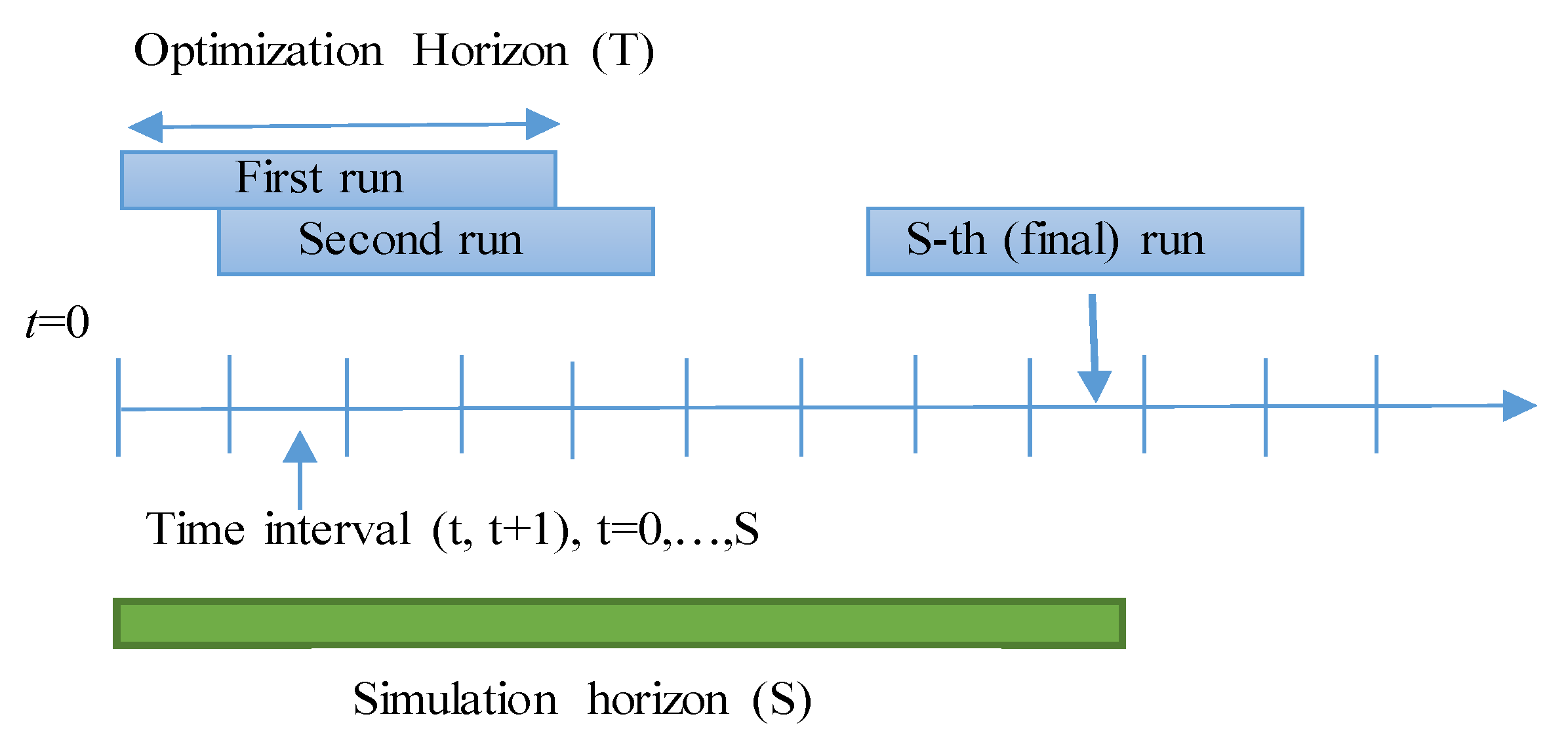
It is important to note that the above two-level optimization procedure is intended to operate within a receding horizon control scheme. In particular, as reported in Figure 2, an optimization horizon (T) is defined over which it is assumed that reliable forecasts about future uncertain inputs and parameters (in this case, power demand, generation from renewables, prices) are available. Such forecasts are provided by prediction models which are considered to be external to the proposed control scheme. Of course, the optimization horizon is the length over which the optimization problem is run. In a receding horizon scheme, in the first run, the optimal control actions for the entire length of the optimization horizon are found, but only the solution corresponding to the first time interval is actually applied. Then, at the beginning of the second time interval, new information from sensors in field (concerning the system state) and updated forecasts of the external inputs are acquired. On this basis, a new optimization run is carried out, and so on until the horizon over which the system is actually operated or simulated (simulation horizon) is completely covered (see Figure 2).
The optimization problem considered in this paper refers to a single iteration of the receding horizon control procedure and is focused on the possibility of efficiently solving the problem via a two-level approach. Clearly, in a receding horizon scheme, at each new time interval, new information is acquired and the two-level optimization procedure is again carried out.

3. The AGG System Model and Optimization Problem

3.1. Representation of the Network Constraints

The considered physical system is composed by buildings and microgrids, both including renewables and storage systems, and connected to the main grid.
In order to formally represent the system model, the following sets are considered:
  • N = { 1 , , n } set of indexes associated to the distribution grid nodes;
  • B = { 1 , , b } set of indexes associated to LUs of type building;
  • M = { b + 1 , , b + m } set of indexes associated to LUs of type microgrid;
  • A = B M set of the indexes associated to all users;
  • H j = { 1 , , h j } set of indexes associated to the cogeneration plants of microgrid j, j M ;
  • R R j = { 1 , , l j } set of indexes associated to the renewable sources of LU j, j A ;
  • R j = { 1 , , r j } set of indexes associated to rooms in building j, j B .
It is necessary to consider the power flow equations for active and reactive power, which affect the power exchanges among LUs connected to the grid. As in [29,30], in the linearized form and in discrete time, these equations can be expressed as follows
p u , z , t = G u , z ( v u , t v z , t ) + B u , z ( δ u , t δ z , t ) u , z N , u z , t = 0 , , T 1
q u , z , t = B u , z ( v u , t v z , t ) G u , z ( δ u , t δ z , t ) u , z N , u z , t = 0 , , T 1
where:
  • G u , z and B u , z are conductance and susceptance parameters for line ( u , z ) ;
  • v u , t and δ u , t are the voltage magnitude and phase at node u, respectively;
  • p u , z , t and q u , z , t are the active and the reactive power flows (from u to z), respectively.
T is the number of time intervals considered, that is, the optimization horizon.
The quantities v u , t , p u , z , t and q u , z , t , are a-dimensional and are expressed with reference to a common voltage/power base value (i.e., as p. u. values).
The balance equation for active power at each node p is given by
j A C O N N u , j D j , t + z N z u P u , z , t = 0 u N , u 1 ,   t = 0 , , T 1
where C O N N u , j is equal to 1 if the LU j is directly connected to u and 0 otherwise. D j , t is the power flow [kW] to the j-th LU from the unique node to which is connected (assumed positive if it is sent to the user j). P u , z , t is the power flow [kW], unrestricted in sign, from node u to node z (i.e., the p.u. value ( p u , z , t ) multiplied by the base value).
Note that (3) holds for u 1 . In fact, conventionally node 1 is defined as the connection node to the main grid, to which no LU is directly connected. For this node, instead of (3), the following equation holds:
z N z 1 P 1 , z , t P g r i d , t = 0 t = 0 , , T 1
where P g r i d , t is the power flow [kW] between node 1 and the main grid (considered as positive when the power is entering the node).
Similarly, the balance equation for reactive power is given by:
j A C O N N u , j Q j , t + z N z u Q u , z , t = 0 u N , u 1 ,   t = 0 , , T 1
where Q j , t is the reactive power exchange [kvar] between node u and the LUs and Q p , q , t represents reactive power flows from node u to node z. In this case too, node 1 has a different equation, namely:
z N z 1 Q 1 , z , t Q g r i d , t = 0 t = 0 , , T 1
where Q g r i d , t is the reactive power flow [kvar] between node 1 and the main grid.
In this model, the following constraints must be fulfilled:
v u M I N v u , t v u M A X u N ,   t = 0 , , T 1
Q g r i d M I N Q g r i d , t Q g r i d M A X t = 0 , , T 1
P g r i d M I N P g r i d , t P g r i d M A X t = 0 , , T 1
D j M I N D j , t D j M A X j A ,   t = 0 , , T 1
Q j M I N Q j , t Q j M A X j A ,   t = 0 , , T 1
where the upper and lower bounds have a straightforward meaning.
It is supposed that the AGG only requests for a variation (decrease) of active power. To this end, the AGG, in order to determine incentives and to divide among its customers the (active) load reduction, has to quantify the reductions’ possibilities of each LU using limited information about the local systems’ states. For this reason, an emulation is necessary (i.e., an approximate simulation) of the dynamic behavior of each LU, as described in the following sub-sections.

3.2. Emulation of the LUs Corresponding to Buildings

This subsection reports the model used for the emulation of a building, embedded in the statement of the higher-level problem. This model includes a storage system, renewables, and heat pumps. The state of charge (SOC) dynamics of storage systems (one for each building) can be represented by the following equations
S O C j , t + 1 = l o s s j S O C j , t η j ( P S , j , t ) P S , j , t Δ C A P j j B ,   t = 0 , , T 1
η j ( P S , j , t ) = { η c , j i f P S , j , t < 0 1 / η d , j o t h e r w i s e j B
where C A P j [kWh] is the capacity of the storage in building j, η c , j , η d , j are efficiency parameters [adim] (≤ 1) in charging and discharging modes, l o s s j [adim] is a loss coefficient due to the internal losses and Δ is the time discretization interval [h]. Instead, P S , j , t is the power flow (unrestricted in sign and assumed as positive when energy is drawn from the storage) from/to the storage [kW], and S O C j , t [adim] is the storage state of charge (expressed as a fraction with respect to the capacity).
The electrical balance equation includes the sum of power feeding the building (i.e., power from storage, renewables, power from the main grid) that is equal to the power demand L j , t minus a possible decrease D A G G , j , t [kW] requested by the AGG (being of course D A G G , j , t L j , t ). That is,
P R E S , j , t + P S , j , t + D j , t = L j , t D A G G , j , t j B ,   t = 0 , , T 1
with
L j , t = q H P , j , t + q E , j , t j B ,   t = 0 , , T 1
where P R E S , j , t is the power from renewables for building j, q H P , j , t is the electrical power feeding the heat pumps, and q E , j , t the remaining forecasted electrical load.
As regards reactive power, it is possible to write:
Q R E S , j , t + Q S , j , t + Q j , t = Q F , j , t j B ,   t = 0 , , T 1
where Q R E S , j , t , Q S , j , t , and Q F , j , t are the reactive power [kvar] associated with renewables and storage systems and the forecasted demand, respectively, and Q j , t is the reactive power [kvar] exchange with the main grid.
It is supposed that the AGG has no detailed information about the temperature in the various rooms in each building. Thus, a single variable T j , t [K] is used to represent the temperature of the overall building j. The dynamics of such temperatures is represented as in [31], namely:
T j , t + 1 = T j , t + Δ C T H , j [ η s q H P , j , t 1 R T H , e x t , j ( T j , t T e x t , t ) ] j B ,   t = 0 , , T 1
where C T H , j is the thermal capacitance in building j [kWh/K], T e x t , t is the external temperature [K], η s q H P , j , t is the thermal power [kW] provided by heat pumps, R T H , e x t , j is the thermal resistance [K/kW] between building j and the external environment, and η s [adim] is given by:
η s = σ η s , h e a t ( 1 σ ) η s , c o o l j B
where σ is a given constant specifying whether the heat pump operates in heating mode ( σ = 1 ) or in the cooling mode ( σ = 0 ), and η s , h e a t and η s , c o o l are efficiency parameters [adim].
The following upper and lower bound constraints must be taken into account:
T j M I N T j , t T j M A X j B ,   t = 0 , , T 1
0 q H P , j , t q H P M A X j B ,   t = 0 , , T 1
S O C j M I N S O C j , t S O C j M A X j B ,   t = 0 , , T 1
P S , j , t M I N P S , j , t P S , j , t M A X j B ,   t = 0 , , T 1
Q S , j , t M I N Q S , j , t Q S , j , t M A X j B ,   t = 0 , , T 1
Q R E S , j M I N Q R E S , j , t Q R E S , j M A X j B ,   t = 0 , , T 1
where all bounds for control and state variables are known parameters, being P S , j , t M I N and Q S , j , t M I N negative values. Note that, whereas P R E S , j , t is a given quantity (known at least as a forecast), Q R E S , j , t may be considered as a decision variable since its value may be adjusted, for any time interval, by means of an electronic system based on the use of inverters.
Finally, the following constraints must be satisfied:
D A G G , j , t D A G G , j , t M A X j B ,   t = 0 , , T 1
t = 0 T 1 D AGG , j , t D A G G , T O T , j j B ,
where the upper bounds D A G G , j , t M A X and D A G G , T O T , j are given for each building.

3.3. Emulation of the LUs Corresponding to Microgrids

This subsection presents the model used to emulate microgrids within the statement of the higher-level problem. Microgrids can be modeled in a similar way as for buildings. However, the system model is in this case a bit more complicated because the thermal balance must be considered, given the presence of cogeneration plants in microgrids.
Specifically, the electrical balance is given by:
P R E S , j , t + P S , j , t + P E L , j , t + D j , t = q H P , j , t + q E , j , t D A G G , j , t j M ,   t = 0 , , T 1
Q R E S , j , t + Q S , j , t + Q j , t = Q F , j , t j M ,   t = 0 , , T 1
where P E L , j , t is the power produced from fossil fuel plants.
The thermal balance in the heating operation mode is given by:
P T H , B O I L , j , t + P T H , R E S , j , t + P T H , j , t D H , j , t j M ,   t = 0 , , T 1
where P T H , B O I L , j , t , P T H , R E S , j , t , P T H , j , t represent thermal power from the gas-fed boiler, renewables, and cogeneration plant, respectively, and D H , j , t is the thermal demand for heat.
Instead, in the cooling operation mode, the balance is:
P T H , R E S , j , t + P T H , j , t D H , j , t + P T H , C H I , j , t j M ,   t = 0 , , T 1
where P T H , C H I , j , t is the thermal power needed to feed chillers. Moreover, in the cooling mode, also the following constraints need to be satisfied:
η s , c o o l q H P , j , t + χ P T H , C H I , j , t D C , j , t j M ,   t = 0 , , T 1
where D C , j , t is the cooling power demand, and χ is the efficiency of the chiller [adim].
Besides, also in the case of microgrids, constraints (12),(13) (written of course for j M ) and (20)÷(26) must be fulfilled.
Finally, owing to the finite capacity of the plants, the following upper bounds must be considered:
P E L , j , t P E L M A X j M ,   t = 0 , , T 1
P T H , C H I , j , t P T H , C H I , j M A X j M ,   t = 0 , , T 1

3.4. The Higher-Level Optimization Problem

In this subsection, the statement of the higher-level optimization problem solved by the AGG will be provided. This problem will embed, as constraints, all equations and inequalities that have been introduced in the previous subsections in order to emulate the LUs’ behavior.
The cost function of the higher-level decision problem consists of several terms.
(A)
The first of them is C i n c [€], that is the cost relevant to incentives that must be provided to the LUs in order to diminish their own load. Let C A G G , j , t [€/h], the incentive that the AGG gives to the generic j-th LU per unit time. The following structure of C A G G , j , t as a function of D A G G , j , t is assumed:
C A G G , j , t = a j ( D A G G , j , t ) 2 + b j D A G G , j , t + c j j A ,   t = 0 , , T 1
where a j , b j and c j are given parameters of suitable physical dimension. Then, C i n c can be expressed as:
C i n c = t = 0 T 1 j A C A G G , j , t Δ
(B)
The second term (actually a benefit) is B D R [€], that is the benefit from the external grid due to the load reduction.
To express this term, note that the benefit recieved from the market for the generic time interval is given by a known unit cost C M a r k e t , t [€/kWh] multiplied by the reduction of power D R t [kW] at the point of connection with the main grid. It is supposed that an overall (maximal) reduction M R t t = 0 , , T 1 [kW] has been agreed in advance.
The reduction of power D R t can be formalized as the difference between the forecasted request P g r i d , d a , t (in the day-ahead) and the new actual request P g r i d , t that has to be determined.
That is:
D R t = P g r i d , d a , t P g r i d , t t = 0 , , T 1
It is important to note that P g r i d , d a , t is a given value that cannot be updated, whereas P g r i d , t is a decision variable appearing in (4).
Moreover, if the power reduction is lower than M R t , there is a fee that must be paid. Thus the overall benefit obtained through a set of reductions D R t t = 0 , , T 1 is given by:
B D R = t = 0 T 1 [ C M a r k e t , t D R t C f e e , t ( M R t D R t ) ] Δ
where C f e e , t is a unit cost coefficient [€/kWh]. Namely, this coefficient represents the cost associated to a unit of unsatisfied energy demand. The following constraints hold as regards D R t , namely:
0 D R t M R t t = 0 , , T 1
On this basis, B D R can be written simply as:
B D R = t = 0 T 1 [ ( C M a r k e t , t + C f e e , t ) D R t C f e e , t M R t ]
(C)
Finally, there is a term called “Assignment Fairness” ( C A F [kW2]) that is introduced to avoid too unbalanced power reductions among the population of LUs. This term can be written as:
C A F = t = 0 T 1 j A [ D A G G , j , t D R t L j , t l A L l , t ] 2
At this point it is possible to formalize the overall AGG decision problem as follows.
The higher-level (AGG) decision problem:
m i n J = C i n c B D R + ω C A F
s.t. constraints (1)÷(40) and
α min C M a r k e t , t D A G G , j , t C A G G , j , t α max C M a r k e t , t D A G G , j , t j A ,   t = 0 , , T 1
In the expression of the cost (41), ω [€/kW2] is a tradeoff coefficient whose value should be tuned on the basis of the real case study considered.
Constraint (42) must be inserted in order to avoid excessive discrepancies between the benefit provided by the market to the AGG (with reference to a specific LU j) and the overall incentive provided by the AGG to that LU. In (42) α min and α max are fixed parameters (<1) and represent minimum and maximum fractions of the benefit to the LUs.
Having so represented the optimization problem to be solved by the AGG, we are now in a position to introduce problems that have to be solved by each LU.

4. The LUs’ Optimization Problem

The LUs track the references coming from the solution of the AGG problem, but have detailed local information and may decide how to manage production plants and storage systems in order to accomplish the AGG’s requests.

4.1. The Model Used for the Optimization Problem of a Building

In the detailed model considered for the optimization of a single building, each room is individually considered. The dynamics of the temperature of the i-th room of building j ( T ˜ i , j , t [K]), is represented as:
T ˜ i , j , t + 1 = T ˜ i , j , t + Δ C i , j [ η s q i , j , t 1 R ˜ T H , e x t , i , j A ˜ e x t , i , j ( T ˜ i , j , t T e x t , t ) r R j r i 1 R ˜ T H , i , r , j A ˜ i , r , j ( T ˜ i , j , t T ˜ r , j , t ) ] j B ,   t = 0 , , T 1 ,   i R j
where:
  • C i , j is the thermal capacitance of room i in building j [kWh/K];
  • T e x t , t is external temperature [K];
  • R ˜ T H , e x t , i , j is the thermal resistance between room i in building j and the external environment [k/kW];
  • R ˜ T H , i , r , j is the thermal resistance between room i and room r in building j [K/kW];
  • A ˜ i , r , j is an entry of the adjacency matrix: It is equal to 1 if room i is adjacent to room r and 0 otherwise [adim];
  • A ˜ e x t , i , j is a coefficient equal to 1 if room i is adjacent to external environment and 0 otherwise [adim];
  • η s q i , j , t is the thermal power (unrestricted in sign) provided by heat pumps in room i in building j [kW].
Moreover, let
q ˜ H P , j , t = i R j q i , j , t j B ,   t = 0 , , T 1
where q ˜ H P , j , t has the same physical meaning as q H P , j , t but now it corresponds to the power provided to the heat pumps in building j that is actually determined solving the problem for the detailed model of that building.
Even for the detailed model of the single building the presence of a single storage element is considered, whose dynamics can still be represented via (12)–(13).
The power balance equation is given by:
P R E S , j , t + P ˜ S , j , t + D L U , j , t = L ˜ j , t D A G G , j , t j B ,   t = 0 , , T 1
which has the same meaning as (14) but where:
  • P ˜ S , j , t is the power flow form the storage element corresponding to the solution of the local problem;
  • D L U , j , t is the actual power flow from the main grid to the LU j, determined by the solution of the local problem;
  • L ˜ j , t is the building load, expressed in a more detailed way with respect to (14), that is:
    L ˜ j , t = q ˜ H P , j , t + P v e h , j , t + P w a s h , j , t + q ˜ E , j , t j B ,   t = 0 , , T 1
Including:
-
fixed consumption q ˜ E , j , t ;
-
power necessary to feed electrical vehicles P v e h , j , t ;
-
power necessary to feed washing machines P w a s h , j , t .
However, there is a fundamental difference between (45)–(46) with respect to (14)–(15). In fact, whereas L j , t , q H P , j , t , and q E , j , t are considered as fixed in (14)–(15), quantities L ˜ j , t , P v e h , j , t , and P w a s h , j , t are decision variables within the problem of the LU corresponding to building j. The washing machines (partly) and the electrical vehicle loads are considered as deferrable, provided that the following constraints are fulfilled:
t = 0 T 1 P v e h , j , t Δ = E T O T , v e h , j j B
P w a s h , j , t = P w a s h , j , t f i x + P w a s h , j , t d e f j B ,   t = 0 , , T 1
t = 0 T 1 P w a s h , j , t d e f Δ = E T O T , w a s h , j d e f j B
where E T O T , v e h , j , is the total electrical energy demand for electrical vehicles [kWh]. P w a s h , j , t is the power demand for the washing machines that is split in two terms: one fixed P w a s h , j , t f i x (not adjustable) and one deferrable P w a s h , j , t d e f . E T O T , w a s h , j d e f is the total deferrable energy demand [kWh] for washing machines.

4.2. The Optimization Problem for a Building

Each LU j receives form the AGG, as a part of the solution of its problem, the load reductions D A G G , j , t t = 0 , , T 1 attributed to the specific LU, and the (reference) values D j , t t = 0 , , T 1 , corresponding to the power flow between the grid and that LU. Then, the LU problem can be formalized as the minimization of the quadratic deviation between the sequence D L U , j , t of the actual power flow from the main grid and the LU, and the reference sequence D j , t .
Optimization Problem For The Single Building j
m i n J B , j = t = 0 T 1 ( D L U , j , t D j , t ) 2
s.t. constraints (12)–(13) and (43)÷(49), written for the index j of interest.

4.3. The Model Used for the Optimization Problem of a Microgrid

We consider a model with the following entities: Microturbines (representing the cogeneration plants), photovoltaics, electric vehicles charging stations, heat pumps and chillers. Even for the detailed model of the single microgrid, the presence of a single storage element is considered, whose dynamics can still be represented via (12)–(13).
In this model, the electric power balance is given by:
h H j P E L , h , j , t + l R R j P R E S , l , j , t + P ˜ S , j , t + D L U , j , t = L ˜ j , t D A G G , j , t j M ,   t = 0 , , T 1
L ˜ j , t = q ˜ H P , j , t + q ˜ E , j , t + P v e h , j , t j M
l R R j Q R E S , l , j , t + Q ˜ S , j , t + Q L U , j , t = Q D , j , t j M ,   t = 0 , , T 1
where:
  • P E L , h , j , t is the active power coming from the controllable microturbine h in microgrid j;
  • P R E S , l , j , t is the active power that is injected from local renewable energy sources of kind l;
  • P ˜ S , j , t is the active power (unrestricted in sign) drawn from the storage;
  • D L U , j , t is the power coming from the grid;
  • q ˜ H P , j , t is the power requested by heat pumps;
  • q ˜ E , j , t is the fixed electrical demand;
  • P v e h , j , t is the power consumed by electric vehicles.
Powers P v e h , j , t is considered as a deferrable load and is subject to constraints similar to those in Equation (47).
Furthermore, Q R E S , l , j , t and Q ˜ S , j , t , are the corresponding reactive power flows. Note that it is assumed that it is possible to regulate the reactive power from the controllable microturbines, imposing them as equal to zero. Thus, there is no decision variable corresponding to these powers. Instead, it is assumed that the reactive power coming from the renewable energy sources, as well as the reactive power coming from the storage, can be regulated. Thus, such powers are considered as decision variables. Besides, Q D , j , t is a fixed amount of reactive power corresponding to the heat pumps and the electric load (the reactive power for electric vehicles is assumed to be zero).
Besides, the following constraints must be taken into account:
P E L , h , j , t P E L , h , j M A X j M ,   t = 0 , , T 1
The thermal balance constraints, for the heating mode, correspond to:
P ˜ T H , B O I L , j , t + l R R j P T H , R E S , l , j , t + h H j P T H , h , j , t D H , j , t j M ,   t = 0 , , T 1
whereas, for the cooling mode, the constraints are:
l R R j P T H , R E S , l , j , t + h H j P T H , h , j , t D H , j , t + P ˜ T H , C H I , j , t j M ,   t = 0 , , T 1
η s , c o o l q ˜ H P , j , t + χ P ˜ T H , C H I , j , t D C , j , t j M ,   t = 0 , , T 1
P ˜ T H , C H I , j , t P T H , C H I , j M A X j M ,   t = 0 , , T 1
where:
  • P ˜ T H , B O I L , j , t is the thermal power produced by the (unique) gas-fed boiler;
  • P T H , R E S , l , j , t is the thermal power from the l-th renewable energy source;
  • P T H , h , j , t is the thermal power produced by the h-th co-generative microturbine;
  • P ˜ T H , C H I , j , t is the thermal power consumed by the (unique) chiller;
It is important to note that the thermal balance and the electrical power balance are coupled owing to the presence of co-generative microturbines. Namely, for a given microturbine h, it is assumed that the following relationship holds:
P T H , h , j , t = μ h , j P E L , h , j , t j M ,   t = 0 , , T 1
where μ h , j is a given parameter characteristic of the considered microturbine. More complex relationships could be used instead of (59) but, for the sake of simplicity, in this paper a purely linear model is adopted.

4.4. The Optimization Problem for a Microgrid

Even in this case, the optimization problem can be stated as the minimization of the quadratic deviation of the actual behavior with respect to the reference value given by the upper problem, as regards both active ( D j , t t = 0 , , T 1 ) and reactive ( Q j , t t = 0 , , T 1 ) powers.
Optimization problem for the single microgrid j:
m i n J M , j = t = 0 T ( D L U , j , t D j , t ) 2 + ( Q L U , j , t Q j , t ) 2 j M
s.t. constraints (12)–(13), (47) and (51)÷(59)

5. Application to a Case Study

The developed bi-level architecture has been applied to a case study in the Liguria Region, Italy. In particular, the considered case study is related to Savona Municipality data, which is located in the north western part of Italy. In particular, on the territory, it is already present a microgrid at the campus level [29], which includes heat pumps, buildings and renewables, a laboratory microgrid, and a sustainable building that, with renewables and storage systems, can be operated in islanded mode and considered as a microgrid. Moreover, the municipality is planning to replicate the microgrid in different areas and to constitute an energy community in the context of a so-called “smart city project”. For these areas data have been estimated on the basis of territorial characteristics and the Savona Campus Microgrid.
Specifically, six different local users have been considered. Three of them are building type LUs, while others are microgrid type LUs. Figure 3 shows a scheme of the considered case study. The network is composed by a slack node (i.e., the connection to the main grid, green), plus other 5 (blue) nodes: two with building type LUs connected, and three with microgrid type LUs.
The model has been implemented with the optimization modeling software LINGO and the results are presented in the following sub-sections. Due to the high-computational burden, each problem runs in about 4 to 6 min.

5.1. The Available Data and Demands

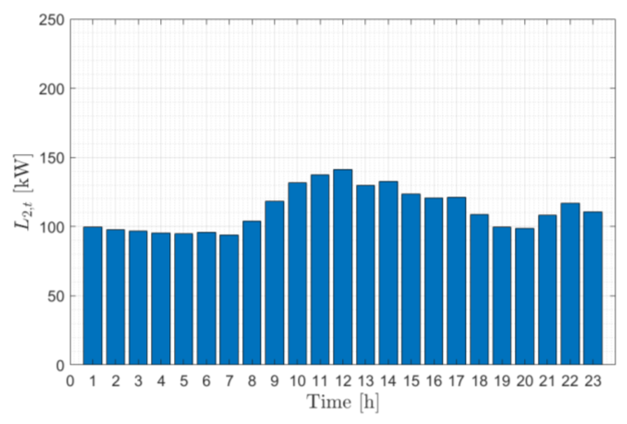
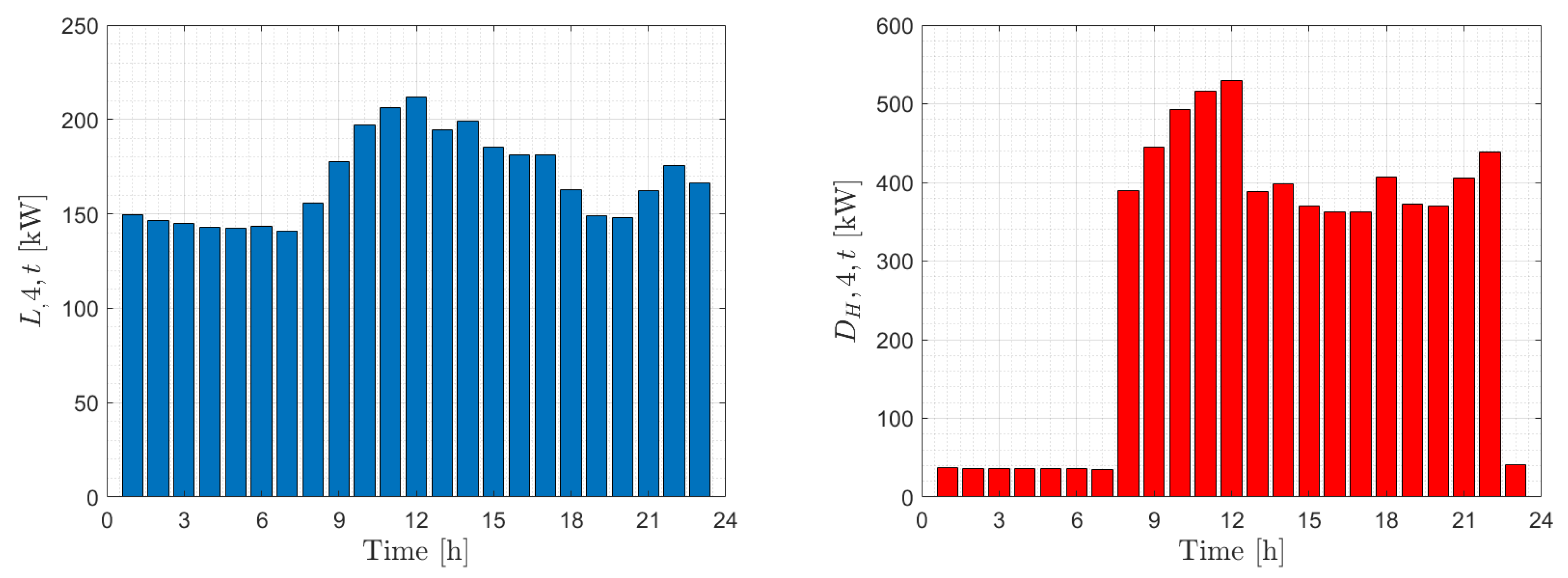
The upper level represents the AGG and emulates the LUs’ behavior in order to determine and distribute the demand reduction. The considered power production from renewables for the different local users (only from PV plants) is reported in Figure 4, while electrical ( L j , t ) and thermal ( D H , j , t ) demands (the latter is considered only for microgrids) of two LUs (one building and one microgrid) are reported in Figure 5 and Figure 6. Electrical and thermal demands for the other LUs have profiles similar to those reported in Figure 5 and Figure 6, respectively. Note that a 24 h optimization horizon has been considered, whereas the time discretization interval is 1 h.

5.2. Results for the AGG Optimization Problem

The optimal results for the AGG’s optimization problem are presented in Figure 7, Figure 8 and Figure 9.
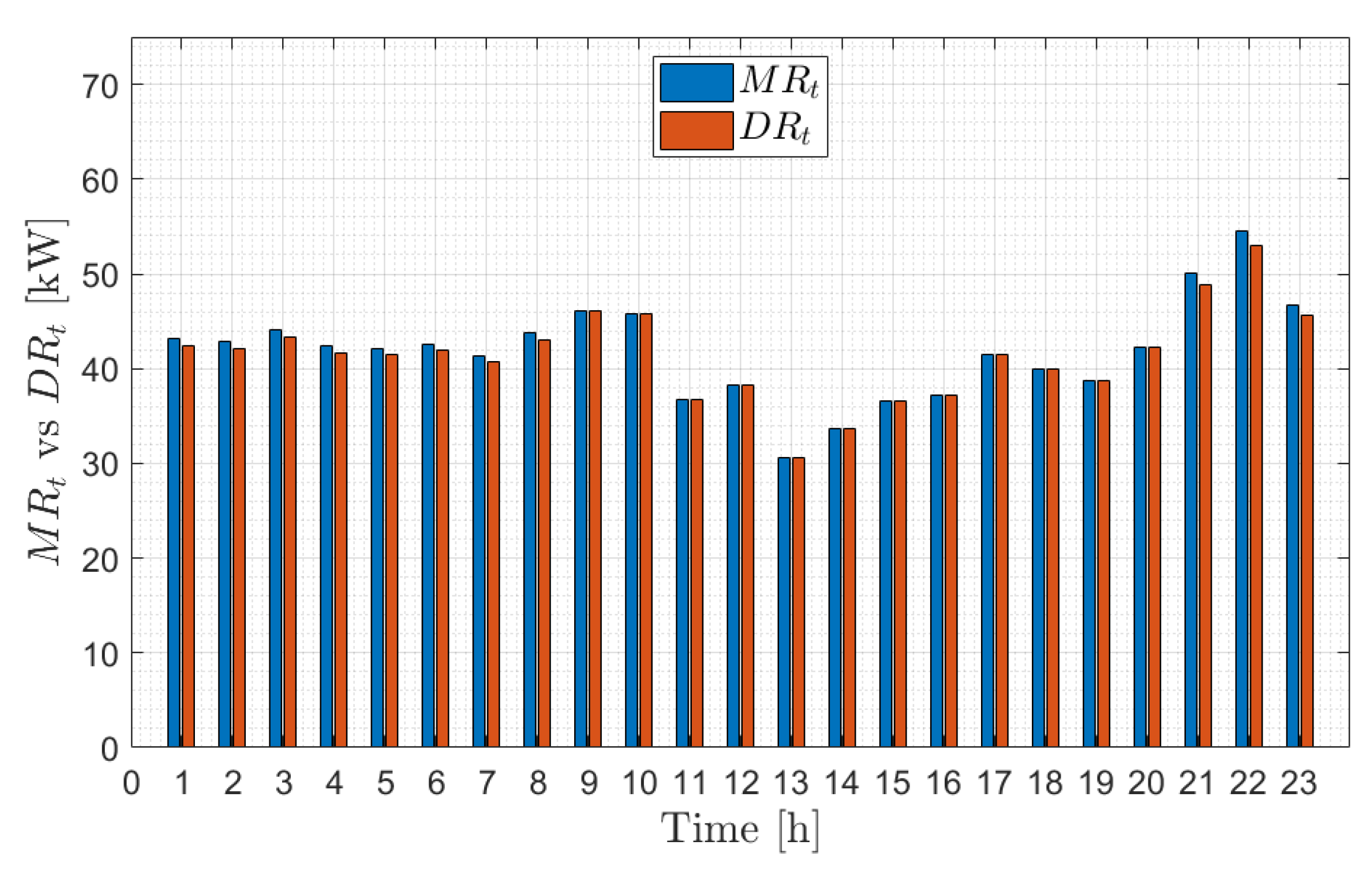
The optimal solution has a power reduction D R t as presented in Figure 7. It highlights that the power reduction requested at the grid node ( M R t ) is almost satisfied along the entire optimization interval, with a slight difference during the first and the last hours due to the absence of renewable power.
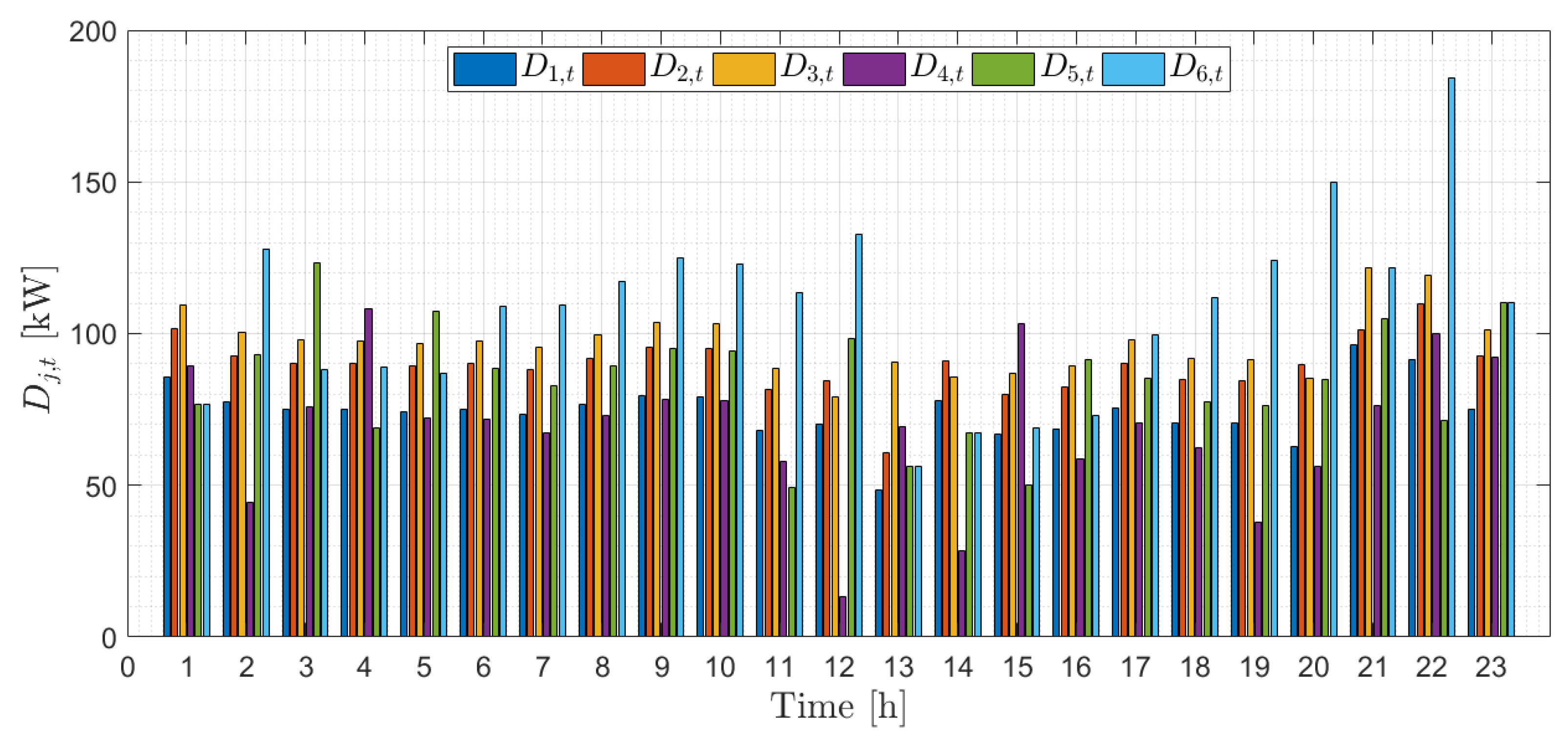
Besides, Figure 8 reports the values for the power exchanged between the main grid and each LU ( D j , t ), while Figure 9 shows the optimal results related to the power reduction D A G G , j , t . It can be noted that the overall power reduction is split in rates which are maintained almost equal along the whole day. This is mainly due to the presence of the “Assignment Fairness” term in the cost function minimized in the higher level problem.
Once the upper-level optimization problem is solved, its solution is used as a reference pattern for the lower-level decision problems.

5.3. Lower-Level Results: Building-Type LUs

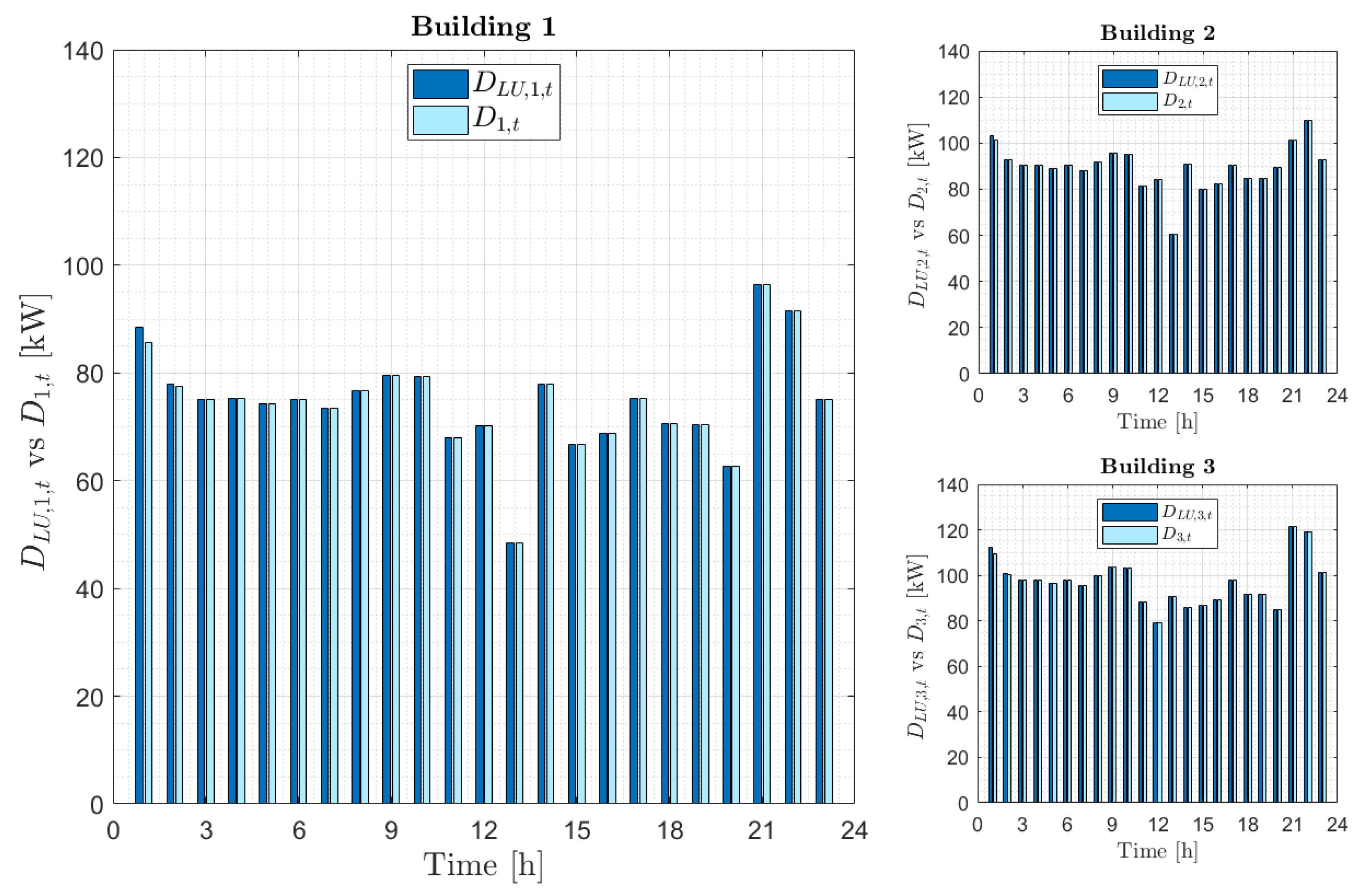
The results of the lower-level optimization problems are presented in Figure 10 and Figure 11. It can be noted that the power reference pattern set by the AGG is tracked almost exactly in the solution of the lower-level problems (Figure 10).
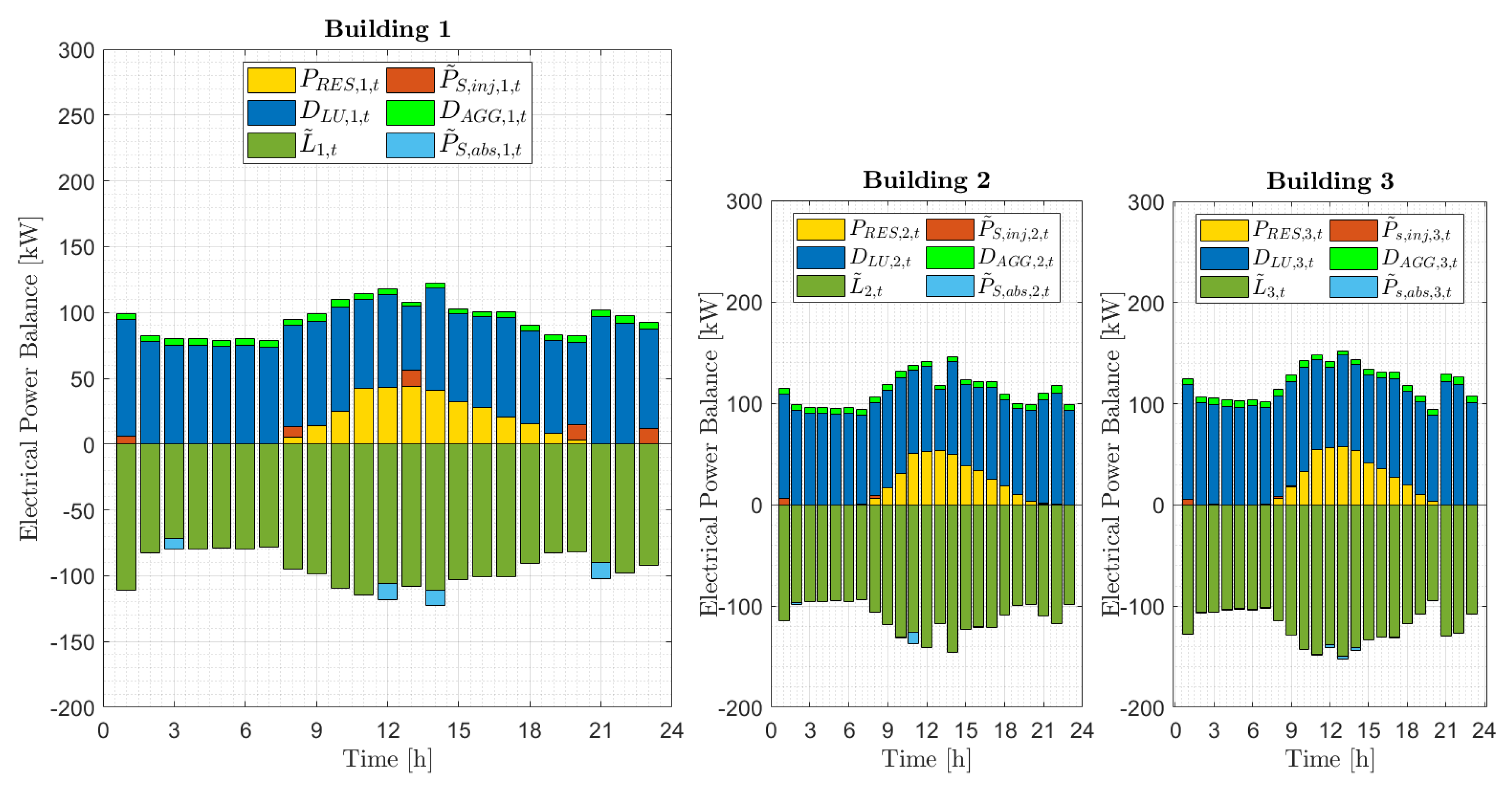
Figure 11 presents the electrical balance (51) at each LU where the largest portion of the load is satisfied by purchasing from the grid since there is not any other power sources but the PV plants and the storage. Note that, for the sake of simplicity in the representation of the power pattern, the power exchanged with the storage P ˜ S , j , t is represented as:
P ˜ S , j , t = P ˜ S , i n j , j , t P ˜ S , a b s , j , t j B ,   t = 0 , , T 1
where P ˜ S , i n j , j , t the first term in the r.h.s. represents the power drawn from the storage and injected into the building, whereas P ˜ S , a b s , j , t represents the power absorbed by the storage.

5.4. Lower-Level Results: Microgrid Type LU

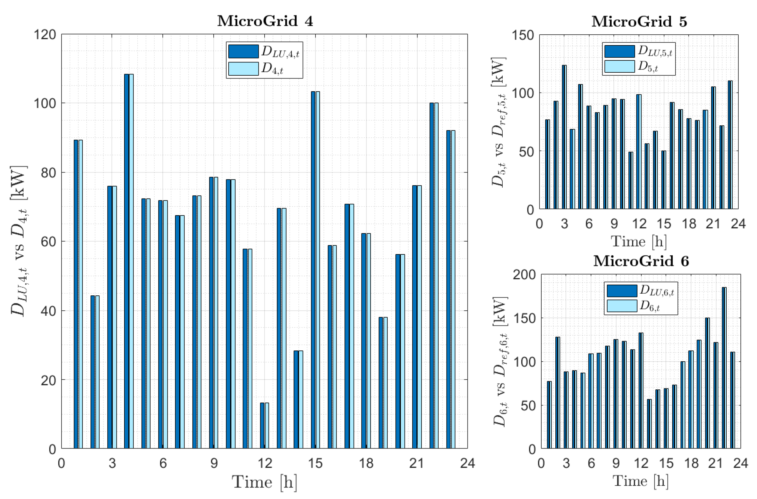
The second type of LUs are microgrids. They have higher flexibility due to the presence of a larger pool of energy production technologies. This leads to a solution (Figure 12) which perfectly fits the reference data.
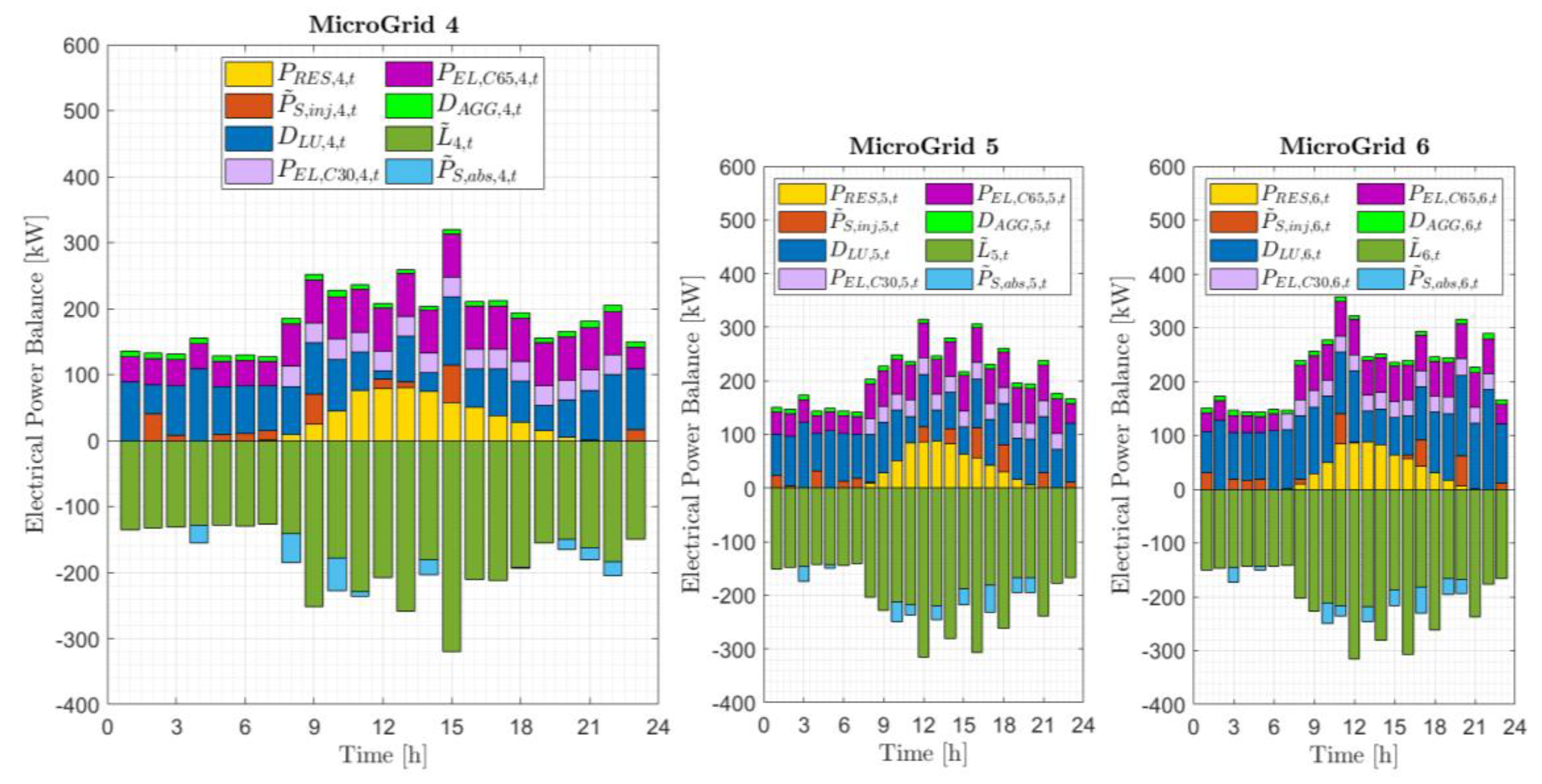
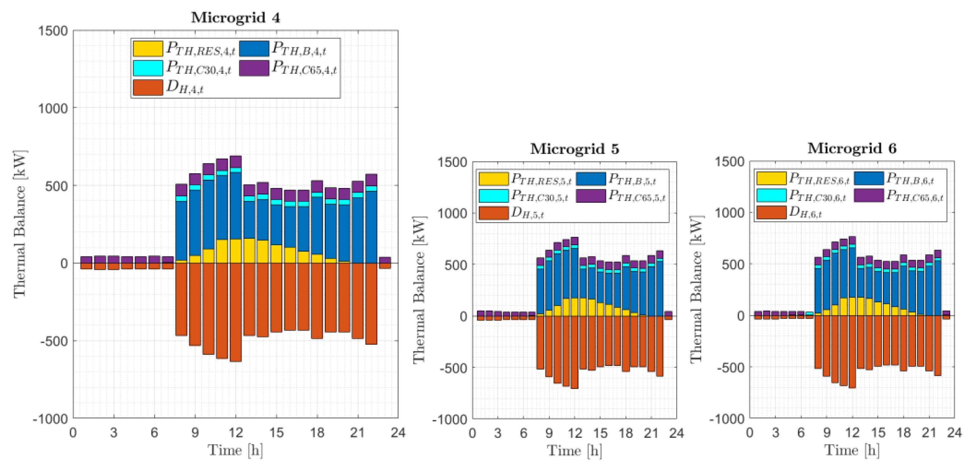
In Figure 13 and Figure 14 both the electrical (51) and thermal balances (56)are reported, highlighting the variety of the energy production pool. Specifically, the presence of two microturbines for each of the three microgrids, one with electrical nominal power of 35 and 65 kW (C30 and C65, respectively). The fraction of the load satisfied through the energy bought from the grid is definitely lower than in the case of buildings because the microturbines are co-generative plants, which are able to satisfy also thermal demands.
As expected, the higher flexibility of the microgrids provides a better solution in regards to the objective function, since the electrical profile totally fits the reference one (see Figure 12).

6. Conclusions

Demand response is a subject of utmost importance and it can provide a noteworthy improvement to the performance of the grid. Of course, this requires the development and the application of viable and effective approaches for energy management. In this framework, an approach was proposed in this paper based on a bi-level architecture in which an AGG of consumers plays the role of a higher-level decision-maker. The problem solved at the AGG level is relevant to the balancing market, and incentives for LUs (i.e., buildings and microgrids) are considered as well as their flexibility. The higher-level, representing the AGG, determines the reference values, to be considered by the LUs, minimizing the overall cost function considered. At the lower level, the local users try to follow the reference values and, through demand response programs, try to contain their costs and to satisfy their demands. The microgrids are characterized by higher flexibility with respect to the other LUs (buildings), owing to the presence of several production plants. The proposed architecture has been developed within the following assumptions in regards to the (bidirectional) interaction between the two levels. First of all, the higher level provides the reference patterns for the lower-level problems. Besides, there is information flow from the lower level to the upper level in regards to the storage initial state and the maximum affordable reduction for each LU. The application of the presented decision scheme could be viewed within a receding-horizon framework, in which, at each time step, only the solution referring to the next time discretization interval is applied. Then, at the next time step, a new solution to the same problem, concerning an optimization interval of the same length as above, is determined after having received the information about the current system state. Further developments will be the implementation of more detailed models for single plants and the use of different renewable energy sources. Another possible extension could the application of the model to grids with different architectures to determine if the load flexibility can be improved.

Author Contributions

Conceptualization, M.R. (Michela Robba), G.F., L.P., R.M. and M.R. (Mansueto Rossi); Methodology, M.R. (Michela Robba), G.F., L.P., R.M. and M.R. (Mansueto Rossi); Software, M.R. (Michela Robba), G.F., L.P., and M.R. (Mansueto Rossi); Validation, M.R. (Michela Robba), G.F., L.P., R.M. and M.R. (Mansueto Rossi); Formal Analysis, M.R. (Michela Robba), G.F., L.P., R.M. and M.R. (Mansueto Rossi); Investigation, M.R. (Michela Robba), G.F. and L.P.; Resources, M.R. (Michela Robba), L.P. and M.R. (Mansueto Rossi); Data Curation, M.R. (Michela Robba), L.P. and M.R. (Mansueto Rossi); Writing-Original Draft Preparation, M.R. (Michela Robba), G.F., L.P., R.M. and M.R. (Mansueto Rossi); Writing-Review & Editing, M.R. (Michela Robba), G.F., L.P., R.M. and M.R. (Mansueto Rossi); Visualization, M.R. (Michela Robba), G.F., L.P., R.M. and M.R. (Mansueto Rossi); Supervision, M.R. (Michela Robba), G.F., L.P., R.M. and M.R. (Mansueto Rossi); Project Administration, M.R. (Michela Robba), R.M.; All authors have read and agreed to the published version of the manuscript.

Funding

This research received no external funding. The outputs of the optimization results have been used as input data for the development of an Energy Management System for sustainable districts that will be developed within the PICK-UP innovation project funded by Liguria Region within the Innovation Pole on Energy Technologies and Sustainable Development (EASS).

Conflicts of Interest

The authors declare no conflict of interest.

Nomenclature

Sets:
T = { 1 , , t } set of time instants;
N = { 1 , , n } set of indexes associated to the distribution grid nodes;
B = { 1 , , b } set of indexes associated to LUs of type building;
M = { b + 1 , , b + m } set of indexes associated to LUs of type microgrid;
A = B M set of the indexes associated to all users;
H j = { 1 , , h j } set of indexes associated to the cogeneration plants of microgrid j, j M ;
R R j = { 1 , , l j } set of indexes associated to the renewable sources of LU j, j A ;
R j = { 1 , , r j } set of indexes associated to rooms in building j, j B .
Decision Variables:
p u , z , t = active power flow for line ( u , z ) at time t [p.u.];
P u , z , t = active power flow for line ( u , z ) at time t [kW];
q u , z , t = reactive power flow for line ( u , z ) at time t [p.u.];
Q u , z , t = reactive power flow for line ( u , z ) at time t [kvar];
v u , t = voltage magnitude at node u at time t [p.u.];
δ u , t = phase magnitude at node u at time t [p.u.];
D j , t = active power exchange from the node u to the LU at time t [kW];
Q j , t = reactive power exchange from the node u to the LU at time t [kvar];
P g r i d , t = active power exchange form the slack node to the main grid at time t [kW];
Q g r i d , t = reactive power exchange from the slack node to the main grid at time t [kvar];
S O C j , t = State of Charge of the storage element j at time t;
Q R E S , j , t = reactive power from renewables of the j-th LU at time t [kvar];
P S , j , t = active power exchange with the storage of the j-th LU at time t [kW];
Q S , j , t = reactive power exchange with the storage of the j-th LU at time t [kvar];
D A G G , j , t = active power decrease requested by the AGG to the j-th LU at time t [kW];
q H P , j , t = electrical power provided by heat pumps in the j-th LU at time t [kW];
L j , t =active power demand of the j-th LU at time t [kW];
T j , t = temperature of the building j at time t [K];
P E L , j , t = power produced from cogeneration plants in microgrid j at time t [kW];
P T H , B O I L , j , t =thermal power produced by the boiler in microgrid j at time t [kW];
P T H , j , t = thermal power produced by the cogeneration plants in microgrid j at time t [kW];
D R t = actual power reduction at the slack node at time t [kW];
C A G G , j , t = incentive that the AGG gives to the generic j-th LU per unit time [€/h];
D L U , j , t = actual power flow (calculated at the lower level) from the grid to the LU j at time t [kW];
T ˜ i , j , t = temperature of the i-th room of building j at time t [K];
q ˜ H P , j , t = same physical meaning as q H P , j , t in the lower-level problem [kW];
P ˜ S , j , t = same physical meaning as P S , j , t in the lower-level problem [kW];
L ˜ j , t = same physical meaning as L j , t in the lower-level problem [kW];
P v e h , j , t = power necessary to feed electrical vehicles in the j-th LU at time t [kW];
P w a s h , j , t = power necessary to feed washing machines in building j at time t [kW];
P w a s h , j , t d e f = deferrable fraction of P w a s h , j , t [kW];
Q L U , j , t = actual reactive power flow (calculated at the lower level) from the grid to the microgrid j at time t [kvar];
P E L , h , j , t = active power coming from the cogenerative microturbine h in microgrid j at time t [kW];
P T H , h , j , t = thermal power produced by the h-th cogenerative microturbine in microgrid j at time t [kW];
P T H , B , j , t = thermal power produced by the (unique) gas-fed boiler in microgrid j at time t [kW];
Q R E S , l , j , t = reactive power coming from the renewable plant l in microgrid j at time t [kvar];
Parameters
G u , z = conductance for line ( u , z ) ;
B u , z = susceptance for line ( u , z ) ;
C O N N u , j = coefficient expressing the connection of LU j and node u;
x M I N = minimum value of a physical quantity x ;
x M A X = maximum value of a physical quantity x ;
Δ = time interval length [h]
P R E S , j , t = active power from renewables of the j-th LU at time t; [kW]
l o s s j = loss coefficient in the storage of the j-th LU;
C A P j = capacity of the storage of the j-th LU [kWh];
η j ( P S , j , t ) = efficiency parameter of the storage of the j-th LU;
η c , j = charging efficiency parameter of the storage of the j-th LU;
η d , j = discharging efficiency parameter of the storage of the j-th LU;
Q F , j , t = reactive power demand of the j-th LU at time t [kvar];
D A G G , T O T , j = maximum active power decrease over the entire day in the j-th LU [kW];
q E , j , t = active power load without the heat pumps in the j-th LU at time t [kW];
T e x t , t = external temperature at time t [K];
C T H , j = thermal capacitance in building j [kWh/K];
R T H , e x t , j = resistance between building j and the external environment [K/kW];
η s =heat pump efficiency coefficient;
η s , h e a t = heat pump efficiency coefficient in heating mode;
η s , c o o l = heat pump efficiency coefficient in heating mode;
σ = constant specifying whether the heat pump operates in heating or cooling mode;
χ = efficiency of the chiller;
P T H , R E S , j , t = thermal power produced by renewables in microgrid j at time t [kW];
D H , j , t = thermal demand (heating) in microgrid j at time t [kW];
D C , j , t = thermal demand (cooling) in microgrid j at time t [kW];
P T H , C H I , j , t = thermal power needed to feed the (unique) chiller in microgrid j at time t [kW];
ω = tradeoff coefficient [€/kW2];
a j = parameter of the cost function of the j-th LU [€/h∙kW2];
b j = parameter of the cost function of the j-th LU [€/kWh];
c j = parameter of the cost function of the j-th LU [€/h];
M R t = overall (maximal) power reduction at the slack node at time t [kW];
P g r i d , d a , t = day-ahead power forecast regarding the slack node at time t [kW];
C M a r k e t , t = benefit from the market for the generic time interval at time t [€/kWh];
C f e e , t = unit cost coefficient at time t [€/kWh];
C i , j = thermal capacitance of room i in building j [kWh/K];
q i , j , t = electrical power provided by heat pumps in room i in building j at time t [kW];
R ˜ T H , e x t , i , j = thermal resistance between room i in building j and the external environment [K/kW];
A ˜ e x t , i , j = entry of the adjacency matrix;
R ˜ T H , i , r , j = is the thermal resistance between room i and room r in building j [K/kW];
A ˜ i , r , j = entry of the adjacency matrix regarding rooms i and r in building j;
q ˜ E , j , t = fixed electrical demand in the lower-level problem in the j-th LU at time t [kW];
E T O T , v e h , j = total electrical energy demand for electrical vehicles in the j-th LU [kWh];
P w a s h , j , t f i x = fixed fraction of P w a s h , j , t [kW];
E T O T , w a s h , j d e f = total deferrable energy demand for washing machines in building j [kWh];
μ h , j = parameter characteristic of the h-th cogenerative microturbine;
P R E S , l , j , t = active power coming from the renewable plant l in microgrid j at time t [kW];
Q D , j , t = fixed amount of reactive power corresponding to the heat pumps and the electric load [kvar];
P T H , R E S , l , j , t = thermal power from the l-th renewable energy source in microgrid j at time t [kW];
Objective function:
J = objective function of the AGG optimization problem;
J ^ B , j = objective function of building j;
J ^ M , j = objective function of microgrid j;
C i n c = cost of providing incentives to the LUs [€];
B D R = benefit from the external grid due to the load reduction [€];
C A F = “Assignment Fairness” [kW2];

References

  1. Carreiro, A.M.; Jorge, H.M.; Antunes, C.H. Energy management systems aggregators: A literature survey. Renew. Sustain. Energy Rev. 2017, 73, 1160–1172. [Google Scholar] [CrossRef]
  2. Hill, C.A.; Such, M.C.; Chen, D.; Gonzalez, J.; Grady, W.M.K. Battery energy storage for enabling integration of distributed solar power generation. IEEE Trans. Smart Grid 2012, 3, 850–857. [Google Scholar] [CrossRef]
  3. Goncalves Da Silva, P.; Ilic, D.; Karnouskos, S. The Impact of Smart Grid Prosumer Grouping on Forecasting Accuracy and Its Benefits for Local Electricity Market Trading. IEEE Trans. Smart Grid 2014, 5, 402–410. [Google Scholar] [CrossRef]
  4. Wang, B.; Sechilariu, M.; Locment, F. Intelligent DC microgrid with smart grid communications: Control strategy consideration and design. IEEE Trans. Smart Grid 2012, 3, 2148–2156. [Google Scholar] [CrossRef]
  5. Grijalva, S.; Tariq, M.U. Prosumer-based smart grid architecture enables a flat, sustainable electricity industry. In Proceedings of the ISGT 2011, Anaheim, CA, USA, 17–19 January 2011; pp. 1–6. [Google Scholar]
  6. Fontenot, H.; Dong, B. Modeling and control of building-integrated microgrids for optimal energy management—A review. Appl. Energy 2019, 254, 113689. [Google Scholar] [CrossRef]
  7. Li, D.; Chiu, W.Y.; Sun, H.; Poor, H.V. Multiobjective optimization for demand side management program in smart grid. IEEE Trans. Ind. Informatics 2018, 14, 1482–1490. [Google Scholar] [CrossRef] [Green Version]
  8. Srinivasan, S.; Palmie, G.; Srinivasan, S.; Palmieri, G.; Del Vecchio, C.; Glielmo, L. Demand Side Management for heating controls in Microgrids. IFAC-PapersOnLine 2016, 49, 611–616. [Google Scholar]
  9. Asensio, M.; Muñoz-Delgado, G.; Contreras, J. Bi-level approach to distribution network and renewable energy expansion planning considering demand response. IEEE Trans. Power Syst. 2017, 32, 4298–4309. [Google Scholar] [CrossRef]
  10. Ferro, G.; Laureri, F.; Minciardi, R.; Robba, M. Optimal Integration of Interconnected Buildings in a Smart Grid: A Bi-level Approach. In Proceedings of the 2017 UKSim-AMSS 19th International Conference on Computer Modelling & Simulation (UKSim), Cambridge, UK, 5–7 April 2017; pp. 155–160. [Google Scholar]
  11. Kovács, A. Bilevel programming approach to demand response management with day-ahead tariff. J. Mod. Power Syst. Clean Energy 2019, 7, 1632–1643. [Google Scholar] [CrossRef] [Green Version]
  12. Jia, Y.; Mi, Z.; Yu, Y.; Song, Z.; Sun, C. A bilevel model for optimal bidding and offering of flexible load aggregator in day-ahead energy and reserve markets. IEEE Access 2018, 6, 67799–67808. [Google Scholar] [CrossRef]
  13. Fernandez-Blanco, R.; Arroyo, J.M.; Alguacil, N.; Guan, X. Incorporating Price-Responsive Demand in Energy Scheduling Based on Consumer Payment Minimization. IEEE Trans. Smart Grid 2015, 7, 817–826. [Google Scholar] [CrossRef]
  14. Najafi, A.; Falaghi, H.; Contreras, J.; Ramezani, M. A Stochastic Bilevel Model for the Energy Hub Manager Problem. IEEE Trans. Smart Grid 2016, 8, 2394–2404. [Google Scholar] [CrossRef]
  15. Feijoo, F.; Das, T.K. Emissions control via carbon policies and microgrid generation: A bilevel model and Pareto analysis. Energy 2015, 90, 1545–1555. [Google Scholar] [CrossRef]
  16. Wei, W.; Wang, D.; Jia, H.; Wang, C.; Zhang, Y.; Fan, M. Hierarchical and distributed demand response control strategy for thermostatically controlled appliances in smart grid. J. Mod. Power Syst. Clean Energy 2017, 5, 30–42. [Google Scholar] [CrossRef] [Green Version]
  17. Bui, V.H.; Hussain, A.; Kim, H.M. A multiagent-based hierarchical energy management strategy for multi-microgrids considering adjustable power and demand response. IEEE Trans. Smart Grid 2018, 9, 1323–1333. [Google Scholar] [CrossRef]
  18. Nazif Faqiry, M.; Das, S. Distributed bilevel energy allocation mechanism with grid constraints and hidden user information. IEEE Trans. Smart Grid 2017, 10, 1869–1879. [Google Scholar] [CrossRef]
  19. Saez-Gallego, J.; Kohansal, M.; Sadeghi-Mobarakeh, A.; Morales, J.M. Optimal Price-Energy demand bids for aggregate price-responsive loads. IEEE Trans. Smart Grid 2018, 9, 5005–5013. [Google Scholar] [CrossRef] [Green Version]
  20. Soares, J.; Canizes, B.; Ghazvini, M.A.F.; Vale, Z.; Venayagamoorthy, G.K. Two-Stage Stochastic Model Using Benders’ Decomposition for Large-Scale Energy Resource Management in Smart Grids. IEEE Trans. Ind. Appl. 2017, 53, 5905–5914. [Google Scholar] [CrossRef]
  21. Shao, C.; Ding, Y.; Wang, J.; Song, Y. Modeling and integration of flexible demand in heat and electricity integrated energy system. IEEE Trans. Sustain. Energy 2018, 9, 361–370. [Google Scholar] [CrossRef]
  22. Asensio, M.; De Quevedo, P.M.; Muñoz-Delgado, G.; Contreras, J. Joint distribution network and renewable energy expansion planning considering demand response and energy storage-part I: Stochastic programming model. IEEE Trans. Smart Grid 2018, 9, 655–666. [Google Scholar] [CrossRef]
  23. Asensio, M.; De Quevedo, P.M.; Muñoz-Delgado, G.; Contreras, J. Joint distribution network and renewable energy expansion planning considering demand response and energy storage-part II: Numerical results. IEEE Trans. Smart Grid 2018, 9, 667–675. [Google Scholar] [CrossRef]
  24. Chen, S.; Cheng, R.S. Operating reserves provision from residential users through load aggregators in smart grid: A game theoretic approach. IEEE Trans. Smart Grid 2017, 10, 1588–1598. [Google Scholar] [CrossRef]
  25. Cheng, P.-H.; Huang, T.-H.; Chien, Y.-W.; Wu, C.-L.; Tai, C.-S.; Fu, L.-C. Demand-side management in residential community realizing sharing economy with bidirectional PEV while additionally considering commercial area. Int. J. Electr. Power Energy Syst. 2020, 116, 105512. [Google Scholar] [CrossRef]
  26. De Zotti, G.; Pourmousavi, S.A.; Morales, J.M.; Madsen, H.; Poulsen, N.K. Consumers’ Flexibility Estimation at the TSO Level for Balancing Services. IEEE Trans. Power Syst. 2019, 34, 1918–1930. [Google Scholar] [CrossRef] [Green Version]
  27. Aghajani, G.R.; Shayanfar, H.A.; Shayeghi, H. Demand side management in a smart micro-grid in the presence of renewable generation and demand response. Energy 2017, 126, 622–637. [Google Scholar] [CrossRef]
  28. Salah, F.; Henriquez, R.; Wenzel, G.; Olivares, D.E.; Negrete-Pincetic, M.; Weinhardt, C. Portfolio design of a demand response aggregator with satisficing consumers. IEEE Trans. Smart Grid 2019, 10, 2475–2484. [Google Scholar] [CrossRef]
  29. Delfino, F.; Ferro, G.; Robba, M.; Rossi, M. An Energy Management Platform for the Optimal Control of Active and Reactive Powers in Sustainable Microgrids. IEEE Trans. Ind. Appl. 2019, 55, 7146–7156. [Google Scholar] [CrossRef]
  30. Bracco, S.; Brignone, M.; Delfino, F.; Pampararo, F.; Rossi, M.; Ferro, G.; Robba, M. An Optimization Model for Polygeneration Microgrids with Renewables, Electrical and Thermal Storage: Application to the Savona Campus. In Proceedings of the 2018 IEEE International Conference on Environment and Electrical Engineering and 2018 IEEE Industrial and Commercial Power Systems Europe (EEEIC/I&CPS Europe), Palermo, Italy, 12–15 June 2018; pp. 1–6. [Google Scholar]
  31. Yao, J.; Costanzo, G.T.; Zhu, G.; Wen, B. Power Admission Control with Predictive Thermal Management in Smart Buildings. IEEE Trans. Ind. Electron. 2015, 62, 2642–2650. [Google Scholar] [CrossRef]
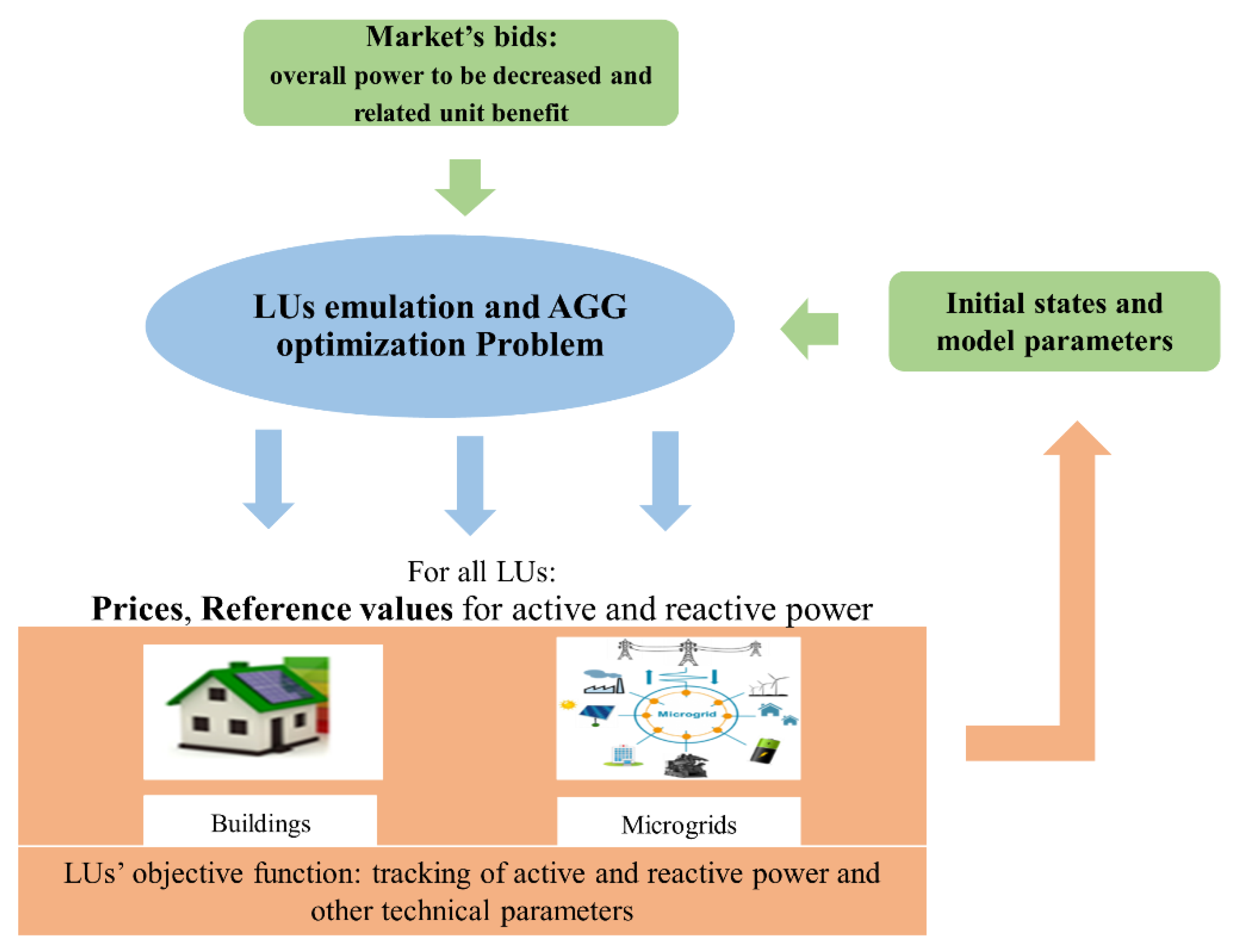
Figure 1. The proposed decision architecture of the Aggregator (AGG)–Local Users (LUs) problem.
Energies 13 01058 g001
Figure 2. A pictorial representation of the receding horizon control scheme.
Energies 13 01058 g002
Figure 3. Network architecture of the case study.
Energies 13 01058 g003
Figure 4. Renewable power production of the LUs.
Energies 13 01058 g004
Figure 5. Electrical demand of the LU number 2 (Building).
Energies 13 01058 g005
Figure 6. Electrical and thermal demand of the LU number 4 (microgrid).
Energies 13 01058 g006
Figure 7. Power reduction at the grid node.
Energies 13 01058 g007
Figure 8. Values of the power exchanged by the LUs and the main grid.
Energies 13 01058 g008
Figure 9. Optimal power reduction resulted from upper-level calculation.
Energies 13 01058 g009
Figure 10. Power exchange between the nodes and the LUs (buildings) compared with their reference values.
Energies 13 01058 g010
Figure 11. Electrical balance in the LUs (buildings).
Energies 13 01058 g011
Figure 12. Power exchange between the nodes and the LUs (microgrids) compared with their reference values.
Energies 13 01058 g012
Figure 13. Electrical balance in the LUs (microgrids).
Energies 13 01058 g013
Figure 14. Thermal balance in the LUs (microgrids).
Energies 13 01058 g014