Dual Closed-Loop Linear Active Disturbance Rejection Control of Grid-Side Converter of Permanent Magnet Direct-Drive Wind Turbine

Abstract

In the permanent magnet direct-drive wind power grid-connected system, in order to solve the coupling problem between $d$-axis and $q$-axis currents and to improve the disturbance rejection performance of direct current (DC) bus voltage under grid faults, a new dual closed-loop structure based on linear active disturbance rejection control (LADRC) is proposed. This new dual closed-loop control includes current inner loop decoupling control and DC bus voltage outer loop control with first-order LADRC. As the LADRC has the advantages of decoupling and disturbances rejection, it is applied to the control of wind power grid-connected inverter. Through analysis, it is demonstrated that the current decoupling control is simpler than proportional integral (PI) control algorithm, the dynamic response speed is faster, and the DC bus voltage control has better anti-disturbance. Finally, a 1.5 MW direct-drive permanent magnet wind power system was established through digital simulation, and the control effects of the two control modes under different working conditions are compared. The simulation results verify that the proposed dual closed-loop control based on first-order LADRC is superior to PI double closed-loop control in terms of decoupling performance and disturbance rejection performance under grid faults.

1. Introduction

At present, the contradiction between the increasing power demand, the shortage of energy supply, and the deteriorating environmental problems makes traditional power generation methods face severe challenges [1,2]. As a clean and pollution-free renewable energy, wind power has the advantages of flexible installation scale, short construction period, high security, and has become a popular power generation method in the new energy field [3]. Permanent magnet direct-drive wind power generation has the advantages of high efficiency, high reliability, and low operation and maintenance costs, and has become a hot topic for scholars at home and abroad [4,5]. At the same time that wind power technology is becoming more mature, the scale of wind power generation systems continues to expand, and the impact on power systems is becoming increasingly apparent. Wind power grid-connected inverter, as the core device connecting wind turbine and grid, plays an important role in stabilizing direct current (DC) bus voltage and controlling grid-side power factor [6]. The control effect of the grid-connected inverter directly affects power quality output from wind turbines. Therefore, research on the control technology of grid-side converter is of great significance for large-scale wind power grid connection.

Double closed-loop structure is usually applied to grid-connected control of grid-side converter in wind power system, that is, voltage outer loop control and current inner loop control [7]. In the double closed-loop control, the steady-state and dynamic characteristics of current control directly affect the performance of voltage loop and even the whole control system, which is the key to converter control. At present, the current control methods are mainly divided into two types: one is indirect current control by controlling alternating current (AC) side voltage of the converter, and the other is direct current control by directly controlling AC side current of the converter [8,9]. The former adopts the open-loop control, with slow dynamic response and sensitivity to system parameters. The latter uses the closed-loop control, which improves the dynamic and static characteristics of the current, as well as the disadvantages that are susceptible to system parameters. Indirect current control has gradually been replaced by direct current control [10,11]. In the direct current control, vector control method is widely used because of its advantages such as fixed switching frequency, low sensitivity to system parameter changes, and good dynamic response characteristics. In wind power systems, grid-side converters usually use grid-voltage-oriented vector control methods [12].

In the dual closed-loop control system of power grid voltage orientation, the bus capacitor voltage controlled by the voltage outer loop is kept at a preset constant value, and the output of the voltage outer loop is used as the reference value of the current inner loop. The current inner loop adjusts the reference value of reactive power according to the requirements of the entire wind power for reactive power, thereby improving the control effect of voltage outer loop [13]. In the typical double-loop control, there is current coupling in inner loop. Traditional voltage feedforward decoupling control can completely eliminate this coupling on the premise of known parameters. However, the parameters of the inverter vary with the working conditions, which leads to incomplete decoupling and poor control effect. In addition, traditional double closed-loop control adopts proportional integral (PI) regulator. The development of science and technology has increasingly higher requirements for control accuracy, response speed, and adaptability to environmental changes. Traditional PI control has gradually revealed its shortcomings [14]. This control method based on error to eliminate errors will produce a certain time delay, integration link will cause phase lag and integral saturation, which is bad for the stability of the system, and PI control has poor anti-interference ability for the system [15], so the effect of traditional dual closed-loop control is not ideal.

Many new control algorithms have been proposed to improve the disadvantages of the traditional dual closed-loop control, perform the decoupling between currents, and improve the control performance of DC bus voltage. In References [16,17], all or part of the high-order terms and coupling terms in the model are ignored directly to design the controller parameters. Although the design of the controller parameters is greatly simplified, the control effect is not very well due to the poor decoupling effect. In Reference [18], a reduced-order method of controlling the inverter side current is proposed to solve the coupling problem. However, there is a phase difference between the final output current and the grid voltage, and the amplitude and phase compensation of the command current are required. In Reference [19], a three closed-loop decoupling control strategy based on state feedback of double inductor current and capacitor voltage to achieve dynamic decoupling is proposed. Reference [20] adopts the deviation decoupling control of the disturbance observer, but there is a steady-state error for the disturbance in the form of acceleration. In Reference [21,22], the method of non-characteristic frequency current injection is used to measure the grid impedance online, and the impedance value is regularly updated to the control loop for decoupling, but it will cause problems such as delay and the injection of sub-harmonics into the grid. Although the above methods can completely eliminate the coupling effect between $dq$ components, the decoupling method is complex and the decoupling quality is dependent on the accurate mathematical model of the object. Considering the uncertainty of the actual system, it is difficult to establish an accurate model, resulting in errors between the theoretical method and the actual system in the control effect, so the above control methods are difficult to be applied to the actual physical system.

However, the actual wind power grid-connected inverter system is a complex system that is nonlinear, strong coupling, multivariable, and easy to be affected by the grid voltage fluctuation [23]. It is difficult to establish an accurate mathematical model, which leads to the unsatisfactory control effect of the traditional control method. Aiming at the uncertain factors such as nonlinear, strong coupling, and large time delay, researcher Han J.Q. proposed the nonlinear active disturbance rejection control (NADRC) technology, an advanced control technology that does not depend on the precise mathematical model of the system, does not need to measure the system’s disturbance, takes the extended state observer (ESO) as the core, observes the actual motion of the system through the input and output of the system, and estimates and compensates the system [15]. However, this kind of nonlinear control method faces many parameters that are difficult to adjust and are not conducive to practical engineering application. Based on this, Professor Gao Z.Q. simplified the structure of the NADRC and proposed a linear active disturbance rejection control (LADRC) method. This linear control method greatly simplifies parameter tuning and reduces the calculation amount [24]. Moreover, the control performance is similar to that of the NADRC, which is of great practical value in engineering. At present, related scholars have applied LADRC to the control of wind power grid-connected inverters and achieved good control results, but few scholars have applied LADRC to the voltage and current double closed-loop control.

This paper takes the direct-drive permanent magnet wind power grid-connected inverter as the research object. Firstly, the mathematical model of the wind power grid-connected inverter and the traditional double closed-loop control system are introduced. The principle and characteristics of traditional first-order LADRC control are analyzed, and voltage and current dual closed-loop control strategy based on first-order LADRC is designed. The effectiveness of the new first-order LADRC dual closed-loop control system designed in terms of decoupling and disturbance rejection is verified by simulation.

2. Control Strategy of Traditional Grid-side Converter

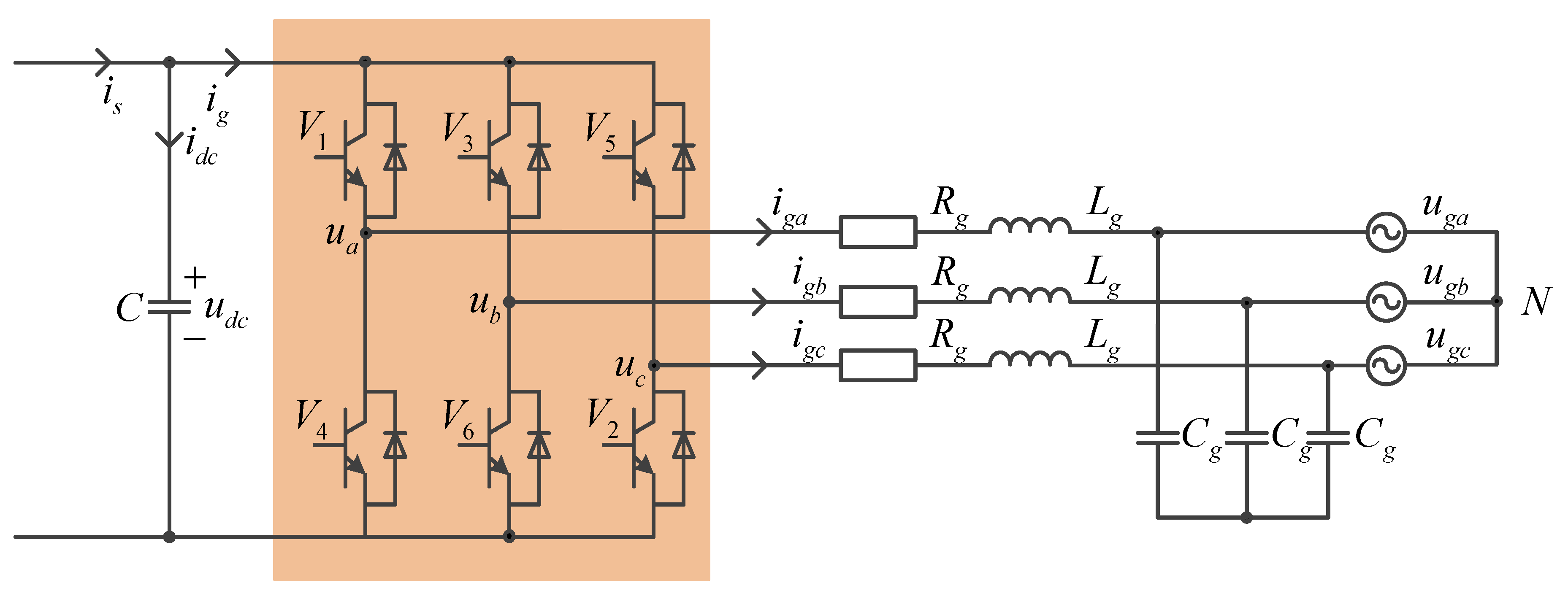
2.1. Mathematical Model of Wind Power Grid-connected Converter

The structure of the permanent magnet direct-drive power generation system is shown in Figure 1. The permanent magnet synchronous generator is connected to power grid through voltage source pulse width modulation (PWM) converters connected back to back. According to the current working conditions and grid requirements, the two PWM converters can run in the state of rectifying or inverting independently. In this kind of AC-DC-AC connection structure, the existence of DC capacitance makes the two converters can be divided into two independent voltage source converters, which can be controlled separately without interference with each other [25,26].

The converter at the grid-side of wind power generation is mainly used to control the power balance of the system, stabilize the DC bus voltage, and generate AC meeting the grid connection conditions. The circuit topology of the grid-side PWM converter is shown in Figure 2, where $C$ is DC bus capacitor, $R_g$ is grid-side equivalent resistance, $L_g$ is AC equivalent filter inductance, and $C_g$ is AC equivalent filter capacitor. $V_i,(i=1,2,3,4,5,6)$ are wholly controlled switching devices insulated gate bipolar transistors (IGBTs) on the six bridge arms of the inverter. $u_a$, $u_b$, and $u_c$ are AC output voltages of the converter, $u_{ga}$, $u_{gb}$, and $u_{gc}$ are three-phase grid voltages, $u_{dc}$ is voltage on the DC bus capacitance, $i_{ga}$, $i_{gb}$, and $i_{gc}$ are output currents of the grid-side converter, $i_s$ is current flowing out of the machine-side converter, $i_{dc}$ is current flowing into DC bus capacitor, and $i_g$ is current flowing into the grid-side inverter.

According to Figure 2, the mathematical model of grid-side inverter in the stationary three-phase coordinate system can be obtained from Kirchhoff’s voltage law. The relationship between voltage and current is as follows:

$$\left[\begin{array}{c}{u}_a\\ u_b\\ u_c\end{array}\right]=\left[\begin{array}{c}{u}_{ga}\\ u_{gb}\\ u_{gc}\end{array}\right]+R_g\left[\begin{array}{c}{i}_{ga}\\ i_{gb}\\ i_{gc}\end{array}\right]+L_g\frac{d}{dt}\left[\begin{array}{c}{i}_{ga}\\ i_{gb}\\ i_{gc}\end{array}\right]$$

(1)

$$C\frac{d{u}_{dc}}{dt}=i_s-i_g=i_s-(S_a{i}_{ga}+S_b{i}_{gb}+S_c{i}_{gc})$$

(2)

where $S_k(k=a,b,c)$ is the switch function, $S_k=0$ represents the upper bridge arm of phase $k$ is in the off state, the lower bridge arm is in the on state, while $S_k=1$ is the opposite of the state of $S_k=0$.

According to Equation (1), the three-phase circuits are independent of each other. By adjusting the inverter output voltages $u_a$, $u_b$, and $u_c$, the AC-side currents $i_{ga}$, $i_{gb}$, and $i_{gc}$ can be changed, so as to realize the control of the inverter. This mathematical model has the advantages of intuitionistic and clear physical meaning, but the disadvantage is that this mathematical model contains time-varying AC, which is not convenient for the design of the control system. The mathematical model of the grid-side inverter in the $dq$ axis rotating coordinate system can be obtained by Park transformation:

$$\left[\begin{array}{c}{u}_d\\ u_q\end{array}\right]=\left[\begin{array}{c}{u}_{gd}\\ u_{gq}\end{array}\right]+R_g\left[\begin{array}{c}{i}_{gd}\\ i_{gq}\end{array}\right]+\omega L_g\left[\begin{array}{c}-i_{gq}\\ i_{gd}\end{array}\right]+L_g\frac{d}{dt}\left[\begin{array}{c}{i}_{gd}\\ i_{gq}\end{array}\right]$$

(3)

$$C\frac{d{u}_{dc}}{dt}=i_s-\frac{3}{2}(S_d{i}_{gd}+S_q{i}_{gq})$$

(4)

where $u_d$ and $u_q$ are the components of grid-side converter output voltage on the $dq$ axis, $u_{gd}$ and $u_{gq}$ represent components of grid voltage on the $dq$ axis, $i_{gd}$ and $i_{gq}$ are the components of grid-side converter output current on the $dq$ axis, $\omega$ is the fundamental angular velocity of the grid voltage, and $S_d$ and $S_q$ are the components of the switch function on the $dq$ axis.

From Equations (3) and (4), it can be known that through coordinate transformation, the AC quantities in $abc$ three-phase stationary coordinate system can be transformed into the DC quantities in $dq$ two-phase rotating coordinate system. By controlling the DC quantities, the AC quantities can be controlled, which brings convenience to the analysis and design of the system.

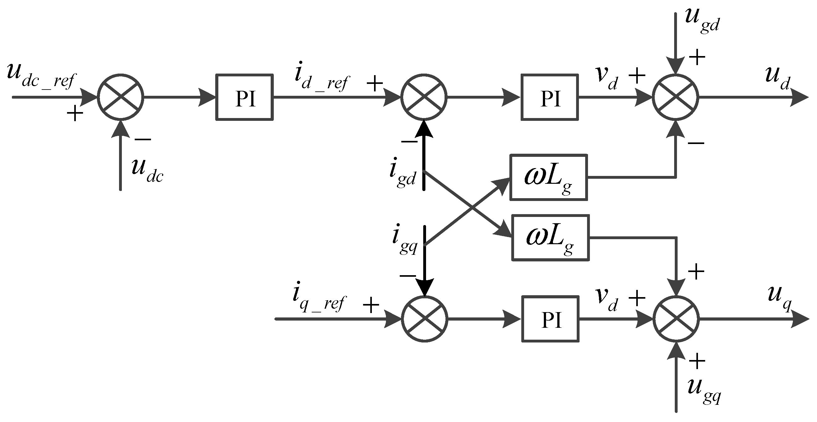
2.2. Control Strategy of Dual closed-loop Grid-Side Converter Based on PI Control

In the control of grid-side converter of the wind power system, the outer loop is adjusted according to the error between the feedback of DC bus voltage and the given value to stabilize the DC bus voltage. The output of the outer loop is used as the reference value of the $d$-axis current of the inner loop, the inner loop closely tracks the input voltage waveform, limits the current command of the current inner loop, and plays a role of overcurrent protection for the system [27].

In synchronous $dq$ coordinates, the grid voltage vector is oriented on the $d$-axis. According to instantaneous power theory, the active power and reactive power output by the inverter are:

$$\{\begin{array}{c}P=3/2·u_{gd}{i}_{gd}\\ Q=3/2·u_{gd}{i}_{gq}\end{array}$$

(5)

The instantaneous value of DC-side input power can be expressed as $P=u_{dc}{i}_{dc}$. Neglecting the power loss of power electronic device, there is $P=u_{dc}{i}_{dc}=3/2·u_{gd}{i}_{gd}$. It can be seen that the voltage $u_{dc}$ on the DC side of the inverter is proportional to the $d$-axis component $i_{gd}$ of the inverter output current. The control of the DC-side voltage $u_{dc}$ can be achieved by controlling the active power, that is, by controlling $i_{gd}$. When PI control is adopted for both voltage and current loops, the analysis process is as follows [28]:

From the Equation (3), $dq$ axis components are coupled, that is, the component that the d-axis is coupled to the $q$-axis is $\omega L_g{i}_{gd}$ and the component that the $q$-axis is coupled to the $d$-axis is $-\omega L_g{i}_{gq}$, which makes it difficult to design the current controllers of $d$-axis and $q$-axis. Decoupling control is needed, and the equation of Equation (3) is slightly changed to:

$$R_g\left[\begin{array}{c}{i}_{gd}\\ i_{gq}\end{array}\right]+L_g\frac{d}{dt}\left[\begin{array}{c}{i}_{gd}\\ i_{gq}\end{array}\right]=\left[\begin{array}{c}{u}_d\\ u_q\end{array}\right]-\left[\begin{array}{c}{u}_{gd}\\ u_{gq}\end{array}\right]+\omega L_g\left[\begin{array}{c}{i}_{gq}\\ -i_{gd}\end{array}\right]$$

(6)

Suppose $\left[\begin{array}{c}{v}_d\\ v_q\end{array}\right]=\left[\begin{array}{c}{u}_d\\ u_q\end{array}\right]-\left[\begin{array}{c}{u}_{gd}\\ u_{gq}\end{array}\right]+\omega L_g\left[\begin{array}{c}{i}_{gq}\\ -i_{gd}\end{array}\right]$, according to Equation (6), the following is obtained:

$$R_g\left[\begin{array}{c}{i}_{gd}\\ i_{gq}\end{array}\right]+L_g\frac{d}{dt}\left[\begin{array}{c}{i}_{gd}\\ i_{gq}\end{array}\right]=\left[\begin{array}{c}{v}_d\\ v_q\end{array}\right]$$

(7)

According to Equation (7), when $v_d$ and $v_q$ are used as the equivalent current control variables, the d-axis and $q$-axis currents are controlled independently. When PI regulator is used in the current inner loop:

$$\{\begin{array}{l}{v}_d=k_{pi}(i_{d\_ref}-i_d)+k_{ii}{\displaystyle \int (i_{d\_ref}-i_d)}dt\\ v_q=k_{pi}(i_{q\_ref}-i_q)+k_{ii}{\displaystyle \int (i_{q\_ref}-i_q)}dt\end{array}$$

(8)

where $k_{pi}$ and $k_{ii}$ are the PI coefficients of the current loop. Due to the introduction of current state feedback, $dq$ axis current has been independently controlled. It is concluded that the decoupling control of the current inner loop of three-phase inverter is based on the feedforward control algorithm, that is to say, the PI regulation results of each axis current contain other axis current information, the injected component and the coupling amount generated by the control object are the same, and the direction is opposite.

Taking the design of the $d$-axis current regulator as an example, considering the small inertia of the PMW control and the delay of the current inner loop signal sampling, the decoupled $d$-axis current inner loop structure is shown in Figure 3 as follows:

In Figure 3, $k_{PWM}$ is the equivalent gain of bridge PWM, $T_s$ is the current sampling period, and PI regulator is written in the form of Pole-Zero, that is, $k_{pi}+k_{ii}/s=k_{pi}({\tau }_{i}s+1)/{\tau }_{i}s$. Since the current sampling period $T_s$ is small, $T_s$ can be combined with a small time constant of $0.5T_s$ to simplify the analysis. When the following performance of the system is mainly considered, the pole of the transfer function of the current control object cancels the zero point of the PI regulator, that is, ${\tau }_i=L_g/R_g$, and the disturbance of $u_{gd}$ is ignored to simplify the analysis. The open-loop transfer function of the current inner loop is obtained:

$$G_i(s)=\frac{k_{pi}{k}_{PWM}}{R_g{\tau }_{i}s(1.5T_{s}s+1)}$$

(9)

According to the parameter setting relationship of the typical I-type system, the PI parameters can be obtained by taking the damping ratio of the system as 0.707:

$$\{\begin{array}{c}{k}_{pi}=\frac{R_g{\tau }_i}{3T_s{k}_{PWM}}\\ k_{ii}=\frac{R_g}{3T_s{k}_{PWM}}\end{array}$$

(10)

The closed-loop transfer function of the current inner loop is:

$${\phi }_i(s)=\frac{k_{pi}{k}_{PWM}/1.5T_s{R}_g{\tau }_i}{s^2+1/1.5T_s·s+k_{pi}{k}_{PWM}/1.5T_s{R}_g{\tau }_i}$$

(11)

When the switching frequency is high enough, ignore the term $s^2$ to get the simplified transfer function of current inner loop:

$${\phi }_i(s)=\frac{1}{3T_{s}s+1}$$

(12)

Equation (12) shows that when the current loop can be approximately equivalent to a first-order inertial link with a time constant of $3T_s$, good following performance, and fast dynamic response, but the system has poor anti-interference ability and there is a certain degree of contradiction between the design of system tracking and anti-interference.

Based on the schematic diagram of the PWM inverter current inner-loop decoupling control, the introduction of DC voltage feedback and a PI regulator without static difference, a double closed-loop control system of three-phase voltage type inverter is formed. The schematic diagram is shown in Figure 4.

3. Design and Frequency Domain Analysis of LADRC

The LADRC is mainly composed of three parts: linear tracking differentiator (LTD), linear extended state observer (LESO), and linear state error feedback control law (LSEF). Among them, LTD arranges the transition process, tracks the input signal, and extracts the differential signal; LESO estimates the state of the object and the total disturbance of the system; and LSEF synthesizes the compensation of disturbance estimator to generate the control signal.

3.1. Design of First-order LADRC

LADRC can treat external disturbances, parameter uncertainty, and coupling as total disturbances; LESO estimates the total disturbances, and the system is compensated for pure integral series by dynamic compensation. Then, use LESF to transform the integral series system into the desired closed-loop system, and obtain desired closed-loop dynamic characteristics. The quality of the LESO directly affects the control performance of LADRC. Therefore, the design of the LESO occupies a very important position in the design of the LADRC and is the core technology of LADRC [29]. Because LADRC does not need to rely on the specific mathematical model of the controlled object, the differential equation of the controlled object can be written as the following general form:

$$\dot{y}=-a_{0}y+w+bu$$

(13)

where $u$ and $y$ are input and output of the system, $w$ is unknown external disturbance, $a_0$ is parameter of the system, $b$ is unknown input control gain, and assuming the estimated value is $b_0$. Set $x_1=y$, define $f(y,w)=-a_{0}y+w+(b-b_0)u$ as the generalized disturbance of the system, including all uncertain factors and unknown external disturbances in the system, and set $x_2=f(y,w)$, $h=f(y,w)$, the state equation of the system can be described as:

$$\left[\begin{array}{c}{\dot{x}}_1\\ \begin{array}{l}{\dot{x}}_2\\ y\end{array}\end{array}\right]=\left[\begin{array}{cc}0& 1\\ \begin{array}{l}0\\ 1\end{array}& \begin{array}{l}0\\ 0\end{array}\end{array}\right]\left[\begin{array}{c}{x}_1\\ x_2\end{array}\right]+\left[\begin{array}{cc}{b}_0& 0\\ 0& 1\\ 0& 0\end{array}\right]\left[\begin{array}{c}u\\ h\end{array}\right]$$

(14)

A second-order LESO is established:

$$\left[\begin{array}{c}{\dot{z}}_1\\ {\dot{z}}_2\end{array}\right]=\left[\begin{array}{cc}-{\beta }_1& 1\\ -{\beta }_2& 0\end{array}\right]\left[\begin{array}{c}{z}_1\\ z_2\end{array}\right]+\left[\begin{array}{cc}{b}_0& {\beta }_1\\ 0& {\beta }_2\end{array}\right]\left[\begin{array}{c}u\\ y\end{array}\right]$$

(15)

where $z_1$ is tracking signal of $y$, $z_2$ is total disturbance signal of tracking, and ${\beta }_1$ and ${\beta }_2$ are the coefficients of the observer. The state variables of the observer can track the state variables of the system in real-time by selecting appropriate parameters.

Take the control law of the system as follows:

$$u=\frac{-z_2+u_0}{b_0}$$

(16)

Ignoring the estimation error of $z_2$ to $f(y,w)$, the system of Equation (15) can be simplified as an integration link:

$$\dot{y}=x_2+b_{0}u=x_2+(-z_2+u_0)\approx u_0$$

(17)

Since there is no observation of the state differential, LSEF adopts proportional control. The proportional control law is:

$$u_0=k_p(v-z_1)$$

(18)

where $k_p$ is the proportional control gain. According to Equation (17) and Equation (18), the transfer function of the closed-loop system is:

$$\phi (s)=\frac{k_p}{s+k_p}=\frac{1}{1/k_p·s+1}$$

(19)

According to Equation (19), the bandwidth of proportional control is ${\omega }_c=k_p$, and the system can be stabilized by selecting the appropriate proportional gain.

In order to avoid high-frequency chatter after the system enters into a steady state due to adding LTD. The LADRC is composed of LESO and LSEF, that is, the LADRC of the system represented by Equation (13) consists of Equations (15), (16), and (18). Its structure is shown in Figure 5:

According to the pole configuration, the pole of Equation (15) is arranged on the bandwidth of the observer:

$$\lambda (s)=s^2+{\beta }_{1}s+{\beta }_2={(s+{\omega }_0)}^2$$

(20)

The gain of the second-order LESO can be obtained:

$${\beta }_1=2{\omega }_0,{\beta }_2={\omega }_0{}^2$$

(21)

Therefore, the first-order LADRC can be simplified as the control of observer bandwidth ${\omega }_0$ and controller bandwidth ${\omega }_c$, and the better control effect can be obtained by adjusting these two parameters reasonably.

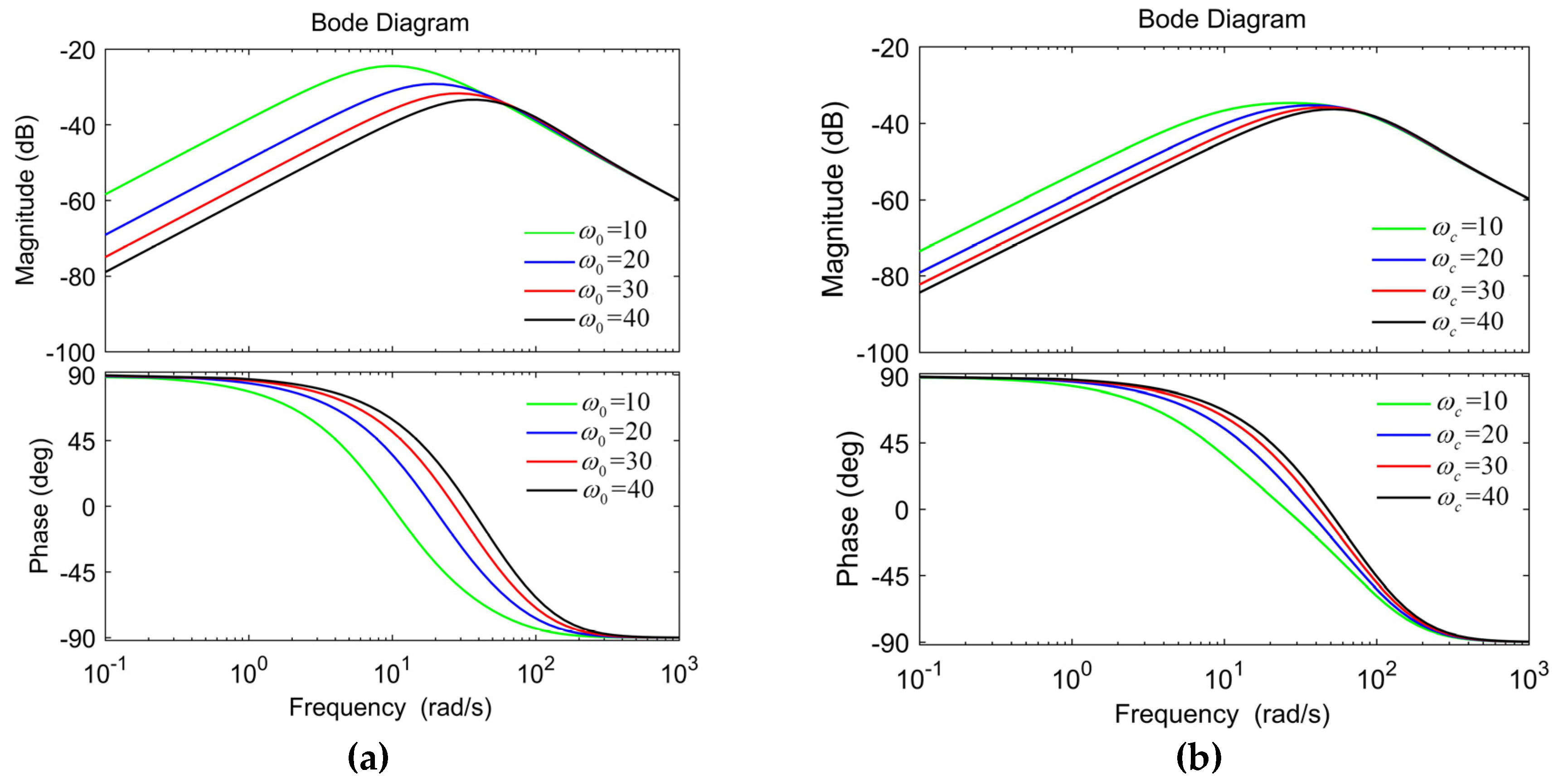
3.2. Frequency Domain Analysis of the First-order LADRC

The LESO is the core of LADRC technology and its tracking estimation ability is the key to affect the performance of LADRC. Therefore, it is analyzed firstly [30].

3.2.1. Convergence and Estimation Error Analysis of Second-order LESO

By substituting Equation (21) into Equation (15) and converting it into the form of transfer function:

$$\{\begin{array}{c}{Z}_1(s)=\frac{{{\omega }_0}^2+2{\omega }_{0}s}{{(s+{\omega }_0)}^2}Y(s)+\frac{b_{0}s}{{(s+{\omega }_0)}^2}U(s)\\ Z_2(s)=\frac{{{\omega }_0}^{2}s}{{(s+{\omega }_0)}^2}Y(s)-\frac{b_0{{\omega }_0}^2}{{(s+{\omega }_0)}^2}U(s)\end{array}$$

(22)

In the Equation (22), $Z_1(s)$, $Z_2(s)$, $Y(s)$, and $U(s)$ are Laplace transforms of $z_1(t)$, $z_2(t)$, $y(t)$, and $u(t)$, respectively.

Set $E_1(s)=Z_1(s)-Y(s)$, $E_2(s)=Z_2(s)-X_2(s)$, the following is obtained:

$$E_1(s)=-\frac{s^2}{{(s+{\omega }_0)}^2}Y(s)+\frac{b_{0}s}{{(s+{\omega }_0)}^2}U(s)$$

(23)

$$E_2(s)=-\frac{s^2(s+2{\omega }_0)}{{(s+{\omega }_0)}^2}Y(s)+\frac{b_{0}s(s+2{\omega }_0)}{{(s+{\omega }_0)}^2}U(s)$$

(24)

For the convenience of analysis, set $Y(s)=U(s)=K/s$, where $K$ is constant, and the steady-state error can be obtained:

$$\{\begin{array}{c}{E}_{ss1}(s)=\underset{s\to 0}{\lim }s{E}_1(s)=0\\ E_{ss2}(s)=\underset{s\to 0}{\lim }s{E}_2(s)=0\end{array}$$

(25)

The equation (25) shows that LESO has good convergence and can realize the estimation of the state variables and generalized disturbances without difference.

Further analyzing the dynamic process of second-order LESO, when $b_0=0$, the response of Equation (22) to the step signal $Y(s)=K/s$ is:

$$Z_1(s)=\frac{K}{s}-\frac{K}{s+{\omega }_0}+\frac{K{\omega }_0}{{(s+{\omega }_0)}^2}$$

(26)

Laplace inverse transform is:

$$z_1(t)=K-K(1-{\omega }_{0}t)e^{-{\omega }_{0}t}\hspace{1em} (t\ge 0)$$

(27)

Finding the extreme point of the Equation (27), $t_1=2/{\omega }_0$ can be obtained. Taking the extreme point into Equation (27):

$$z_1(t_1)=K(1+e^{-2})\approx 1.135K$$

(28)

The Equation (28) shows that there is about 13.5% error in the tracking process of $z_1(t)$ to $y$ in the second-order LESO, this is due to the step mutation of the observed signal, which makes the estimation error suddenly larger, resulting in a larger spike in the output of the observer. In the power system, because of the inertia, the output power of the controlled object will not change abruptly, so there will be no serious error in the tracking of state variables by LESO.

3.2.2. Analysis of the Anti-disturbance Characteristics of LADRC

LADRC has a very strong ability to resist disturbance. The design of LADRC is to design the parameters of ${\omega }_0$ and ${\omega }_c$, and then analyze the influence of ${\omega }_0$ and ${\omega }_c$ on control performance [31].

According to Equations (16) and (18):

$$u=\frac{{\omega }_c(v-z_1)-z_2}{b_0}$$

(29)

By Laplace transformation of Equation (29) and substituting it into Equation (22):

$$U(s)=\frac{1}{b_0}\frac{{(s+{\omega }_0)}^2}{s^2+2{\omega }_{0}s+{\omega }_{c}s}[{\omega }_{c}V(s)-\frac{({\omega }_0{}^2+2{\omega }_0{\omega }_c)s+{{\omega }_0}^2{\omega }_c}{{(s+{\omega }_0)}^2}Y(s)]$$

(30)

Set $G_1(s)=\frac{{(s+{\omega }_0)}^2}{s^2+2{\omega }_{0}s+{\omega }_{c}s}$, $H(s)=\frac{({{\omega }_0}^2+2{\omega }_0{\omega }_c)s+{{\omega }_0}^2{\omega }_c}{{(s+{\omega }_0)}^2}$, according to the above Equation, the following simplified block diagram can be obtained:

According to Figure 6, the Equation (13) after Laplace transform can be transformed into:

$$Y(s)=\frac{1}{s}[F(s)+{\omega }_{c}V(s)G_1(s)-Y(s)H(s)G_1(s)]$$

(31)

Taking $G_1(s)$ and $H(s)$ into the Equation (31) and simplifying it, the following is obtained:

$$Y(s)=\frac{s(s+2{\omega }_0+{\omega }_c)}{(s+{\omega }_c){(s+{\omega }_0)}^2}F(s)+\frac{{\omega }_c}{s+{\omega }_c}V(s)$$

(32)

According to Equation (32), the system output consists of two parts: input and disturbance. When the output contains only input terms, the system control performance is determined only by ${\omega }_c$ and has nothing to do with ${\omega }_0$. The larger ${\omega }_c$ is, the faster the tracking speed is, and there is no overshoot in the tracking process. $f(y,w)$ contains external disturbances and system internal uncertainties, which are affected by ${\omega }_c$ and ${\omega }_0$. The frequency-domain characteristic curves of Figure 7a,b are obtained by adjusting the size of ${\omega }_c$ and ${\omega }_0$, respectively.

From the above analysis, it can be seen that with the increase of ${\omega }_0$ and ${\omega }_c$, the disturbance gain will be reduced and the system’s disturbance rejection performance will be enhanced. In particular, taking disturbance $f(y,w)$ as unit step signal, the output response can be obtained according to the Equation (32):

$$Y(s)=\frac{s(s+2{\omega }_0+{\omega }_c)}{(s+{\omega }_c){(s+{\omega }_0)}^2}\frac{1}{s}=\frac{a_1}{s+{\omega }_c}+\frac{a_2}{s+{\omega }_0}+\frac{a_3}{{(s+{\omega }_0)}^2}$$

(33)

where $a_1=\frac{2{\omega }_0}{{({\omega }_0-{\omega }_c)}^2}$, $a_2=\frac{-2{\omega }_0}{{({\omega }_0-{\omega }_c)}^2}$, $a_3=\frac{{\omega }_c+{\omega }_0}{{\omega }_c-{\omega }_0}$.

The Laplace inverse transformation is used to obtain $y(t)$, and find its limit:

$$\underset{t\to \infty }{\lim }y(t)=\underset{t\to \infty }{\lim }(a_1{e}^{-{\omega }_{c}t}+a_2{e}^{-{\omega }_{0}t}+a_{3}t{e}^{-{\omega }_{0}t})=0$$

(34)

The analysis shows that LADRC has a good ability to suppress external disturbances, and the Equation (34) shows that the larger the bandwidth ${\omega }_0$ and ${\omega }_c$, the faster the response attenuation of the system and the shorter the recovery time.

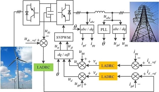
4. Control Strategy of Grid-side Converter Based on LADRC

4.1. Design of Current Inner Loop Control System Based on First-order LADRC

The purpose of current tracking control is to enable the grid-side output current to quickly track the change of the command current. It is a key factor that determines the steady-state and dynamic performance of the converter. The current tracking control method directly determines the accuracy and rapidity of the system.

Considering that when the system is disturbed, the grid-connected point voltage will be affected, which will cause the reference input signal of the current inner loop to contain a disturbance component, and affect the control performance of LADRC. Based on this, the traditional idea of double closed-loop network voltage as feedforward compensation is still adopted to improve the dynamic performance. Taking the $dq$ axis current coupling and parameter uncertainty as the total disturbance, the LESO and LESF are used for estimation and compensation to achieve current decoupling. Taking the $d$-axis current as an example, LADRC is designed. According to Equation (7), it can be seen that:

$$\frac{d{i}_{gd}}{dt}=\frac{1}{L_g}{u}_d+\omega i_{gq}-\frac{R_g}{L_g}{i}_{gd}-\frac{1}{L_g}{u}_{gd}$$

(35)

The mathematical model of the current inner loop control is a first-order system, and the first-order LADRC can be designed. Its state space expression is as follows:

$$\left[\begin{array}{l}\begin{array}{c}{\dot{x}}_{1i}\\ {\dot{x}}_{2i}\end{array}\\ y_i\end{array}\right]=\left[\begin{array}{cc}0& 1\\ \begin{array}{l}0\\ 1\end{array}& \begin{array}{l}0\\ 0\end{array}\end{array}\right]\left[\begin{array}{c}{x}_{1i}\\ x_{2i}\end{array}\right]+\left[\begin{array}{cc}{b}_{0i}& 0\\ 0& 1\\ 0& 0\end{array}\right]\left[\begin{array}{c}{u}_i\\ h_i\end{array}\right]$$

(36)

where $b_{0i}=1/L_g$. $x_{1i}$ is the actual value of $d$-axis current, $u_i$ is reference current $i_{d\_ref}$ of $d$-axis output from the voltage outer loop, $x_{2i}$ is a new state variable expanded by LESO to describe total disturbance of the system, including internal uncertainty and external disturbance of the system, and is recorded as $f_i=-R_g{i}_{gd}/L_g+\omega i_{gq}$ and ${\dot{f}}_i=h_i$.

According to Equations (15) and (21), the second-order LESO of the current inner loop is:

$$\left[\begin{array}{c}{\dot{z}}_{1i}\\ {\dot{z}}_{2i}\end{array}\right]=\left[\begin{array}{cc}-2{\omega }_{0i}& 1\\ {-{\omega }_{0i}}^2& 0\end{array}\right]\left[\begin{array}{c}{z}_{1i}\\ z_{2i}\end{array}\right]+\left[\begin{array}{cc}{b}_{0i}& 2{\omega }_{0i}\\ 0& {{\omega }_{0i}}^2\end{array}\right]\left[\begin{array}{c}{i}_{d\_ref}\\ v_d\end{array}\right]$$

(37)

The linear error feedback control law and disturbance compensation are:

$$\{\begin{array}{c}{u}_{0i}={\omega }_{ci}(i_{d\_ref}-z_{1i})\\ u_i=(-z_{2i}+u_{0i})/b_{0i}\end{array}$$

(38)

According to the previous analysis, PI double closed-loop control and LADRC can be equivalent to the first-order inertia link. The former is $3T_s$ with fixed time constant, and the latter is $1/k_p$ with variable time constant. By controlling the size of $k_p$, the response speed of the inner loop can be controlled.

4.2. Design of Voltage Outer Loop Control System Based on First-order LADRC

The purpose of voltage loop control is to obtain the power needed for inverter and realize the stability of DC side voltage. When voltage outer loop adopts LADRC, its corresponding LESO is established first. According to Equation (4), the mathematical model of the voltage outer loop is a first-order system, and the first-order LADRC can be designed. Its state space expression is:

$$\left[\begin{array}{l}\begin{array}{c}{\dot{x}}_{1u}\\ {\dot{x}}_{2u}\end{array}\\ y_u\end{array}\right]=\left[\begin{array}{cc}0& 1\\ \begin{array}{l}0\\ 1\end{array}& \begin{array}{l}0\\ 0\end{array}\end{array}\right]\left[\begin{array}{c}{x}_{1u}\\ x_{2u}\end{array}\right]+\left[\begin{array}{cc}{b}_{0u}& 0\\ 0& 1\\ 0& 0\end{array}\right]\left[\begin{array}{c}{u}_u\\ h_u\end{array}\right]$$

(39)

where $b_{0u}=-3/2C$. $x_{1u}$ is actual value of bus voltage, $u_u$ is reference value of the DC bus voltage, $x_{2u}$ is new state variable extended by LESO, which is used to describe the total disturbance of the system, including the internal uncertainty and external disturbance of the system. It is recorded as $f_u=i_s/C-3S_q{i}_{gq}/2C$, and ${\dot{f}}_u=h_u$.

According to Equations (15) and (21), the second-order LESO of the voltage outer loop is:

$$\left[\begin{array}{c}{\dot{z}}_{1u}\\ {\dot{z}}_{2u}\end{array}\right]=\left[\begin{array}{cc}-2{\omega }_{0u}& 1\\ -{{\omega }_{0u}}^2& 0\end{array}\right]\left[\begin{array}{c}{z}_{1u}\\ z_{2u}\end{array}\right]+\left[\begin{array}{cc}{b}_{0u}& 2{\omega }_{0u}\\ 0& {{\omega }_{0u}}^2\end{array}\right]\left[\begin{array}{c}{u}_{dc\_ref}\\ i_{d\_ref}\end{array}\right]$$

(40)

By choosing the appropriate observer bandwidth ${\omega }_{0u}$, $z_{1u}$ and $z_{2u}$ can quickly track the DC bus voltage $u_{dc}$ and the total disturbance of the system.

The LESF of proportional control and disturbance compensation link are as follows:

$$\{\begin{array}{c}{u}_{0u}={\omega }_{cu}(u_{dc\_ref}-z_{1u})\\ u_u=(-z_2+u_{0u})/b_0\end{array}$$

(41)

According to the above analysis, the overall block diagram of grid-side converter control is shown in Figure 8:

5. Simulation Analysis

In order to verify the validity and feasibility of the above theoretical analysis, a simulation model of 1.5 MW permanent magnet direct-drive wind turbine grid-connected was established. The simulation was performed from two aspects of reference current step mutation and grid voltage mutation, and the decoupling effect and anti-interference performance of the traditional double closed-loop control and the improved dual closed-loop control based on LADRC are compared. The parameters of the system and controller are given in Appendix A.

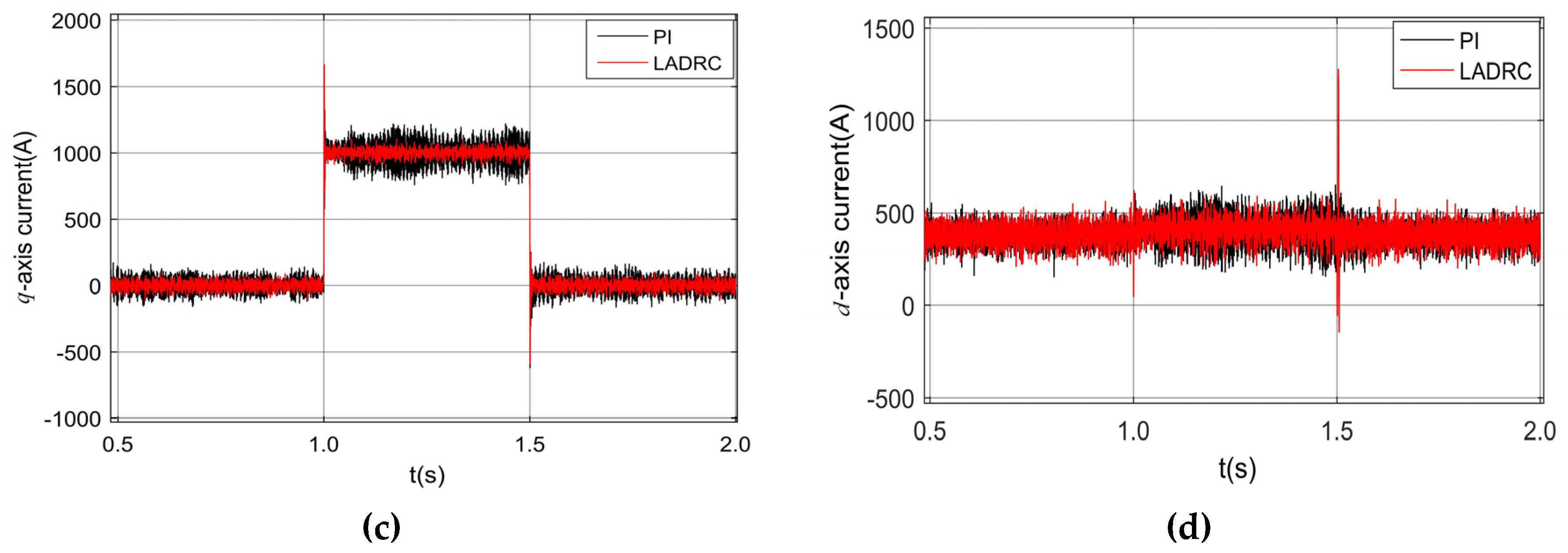
5.1. Simulation Comparison of Current Inner Loop Decoupling Control

When the voltage outer loop adopts PI control, the current inner loop adopts PI control and LADRC, respectively. The $d$-axis reference current increases by 1000 A on the basis of the original reference current at 1 s, and decreases by 500 A at 1.5 s. The simulation diagram of reference current and actual current of $d$-axis and $q$-axis are shown in Figure 9a,b. When q-axis reference current rises from 0 A to 1000 A at 1s and decreases from 1000 A to 0 A at 1.5 s, the waveform diagrams of the $q$-axis and $d$-axis reference currents and actual currents are shown in Figure 9c,d.

It can be concluded from Figure 9 that when the system is in steady-state, PI control and LADRC control can be used in the current inner loop to track the corresponding reference current of $dq$ axis, and the tracking effect of the two controls is no significant difference. However, when the $d$-axis reference current is stepped, the feedforward decoupling control of PI regulator will cause $q$-axis current produce large transient error and transition time, which shows that there is still current coupling in $dq$ axis, and the feedforward decoupling control of PI regulator does not realize the true decoupling. The current decoupling control based on LADRC technology has almost no instantaneous error at the moment of disturbance and keeps stable operation. It shows that the current decoupling control based on LADRC technology can achieve real decoupling. When the $q$-axis reference current changes, the $d$-axis current will oscillate greatly when PI control is used, while LADRC control is adopted, large fluctuations will only occur at the moment of disturbance. It shows that the decoupling effect of the system is better when the latter control is adopted.

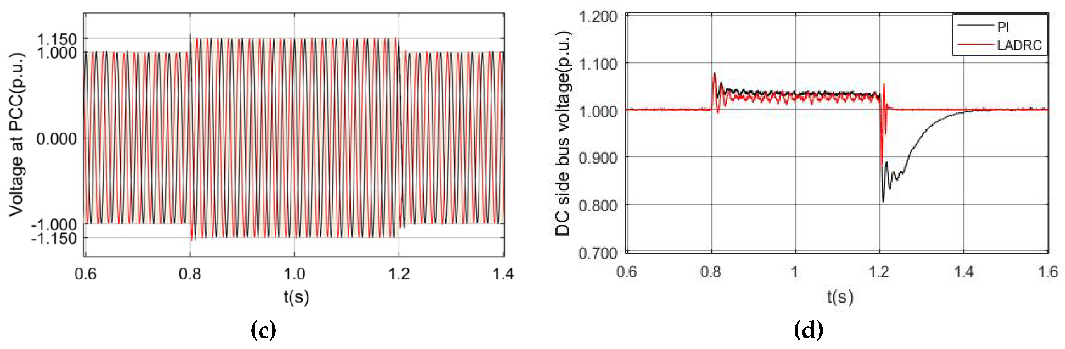
5.2. Simulation Comparison of Voltage Stabilizing Control of Voltage Outer Loop

Current inner loop adopts PI control and voltage outer loop adopts PI control and LADRC, respectively. The waveforms of DC bus voltage when the system is not disturbed are shown in Figure 10a,b.

From Figure 10, it can be seen that when the wind power system is in steady-state operation, and the voltage outer loop adopts PI control, the voltage fluctuation range of DC bus is 0.995 p.u.-1.006 p.u., which reaches a stable state in about 0.3 s. While the fluctuation range based on LADRC is 0.997 p.u.-1.004 p.u., which is stable in about 0.1 s, indicating that the latter control has a fast response speed, high steady-state accuracy, and good tracking performance.

From 0.8 s to 1.2 s, the grid-side voltage drops to 60%. When the above two types of voltage outer loop control are used, the waveform of grid voltage and the waveform of DC bus voltage are shown in Figure 11a,b. Between 0.8 s and 1.2 s, the grid-side voltage increases to 115%. When the two types of voltage outer-loop control are used, the waveforms of grid voltage and DC bus voltage are shown in Figure 11c,d.

As shown in Figure 11, when the grid-side voltage drops by 60%, the voltage fluctuation range of DC bus using LADRC in the voltage outer loop is significantly smaller than the PI control in the voltage outer loop, and the transition process time is shorter. When the grid-side voltage increases by 15%, the dynamic time of the DC bus voltage using LADRC in the voltage outer loop is shorter, which shows that the voltage control with LADRC technology has good anti-interference performance under power grid faults and helps improve the stable operation of the system.

5.3. Comparison between Traditional PI Dual closed-loop Control and LADRC Based Dual closed-loop Control

When traditional PI- and LADRC-based dual closed-loop control are adopted, respectively, $d$-axis reference current increases by 1000 A on the basis of the original reference current at 1 s and decreases by 500 A at 1.5 s. The simulation diagrams of the $d$-axis reference current and the $q$-axis actual current are shown in Figure 12a,b. When $q$-axis reference current rises from 0 A to 1000 A at 1s and decreases from 1000 A to 0 A at 1.5 s, the waveform of $q$-axis reference current and $d$-axis actual current are shown in Figure 12c,d.

Figure 12 also verifies that the decoupling effect of the dual closed-loop control based on LADRC is better than that of the traditional PI control, the use of LADRC in the outer loop can, to some extent, suppress the actual current changes of the $q$-axis and $d$-axis caused by the reference current changes of the $d$-axis and $q$-axis.

When traditional PI- and LADRC-based dual closed-loop control are used, respectively, the waveforms of DC bus voltage under steady-state operation conditions are shown in Figure 13a,b. Under the two control modes, the harmonic distortion rate of the current at grid-connected point is shown in Figure 13c,d.

It can be seen from Figure 13 that under the dual closed-loop control system based on LADRC, the time for the voltage across the capacitor to reach a steady-state is shortened, and the fluctuation range is relatively reduced. From the perspective of waveform distortion rate, the harmonic distortion rate of the grid-connected point current is 3.47% in traditional PI dual closed-loop control strategy, while the harmonic distortion rate of the grid-connected point current is only 1.11% when the dual closed-loop control strategy of LADRC is used. It greatly improves the power quality of the grid-connected point and improves the reliability of the system. In terms of control performance, it shows that the control effect of LADRC is better.

In order to compare the control performance of the above two control methods under grid faults, the simulated grid voltage drops 60% at 0.8 s and returns to normal operation at 1.2 s. The waveforms of the grid-connected point voltage and DC bus voltage are shown in Figure 14a,b. The grid voltage increases by 15% at 0.8 s and returns to normal operation at 1.2 s. The waveforms of the grid-connected point voltage and DC bus voltage are shown in Figure 14c,d. As can be seen from Figure 14, the dual closed-loop control based on LADRC has shorter transient duration, smaller fluctuation range, and better disturbance rejection than that based on PI.

6. Conclusions

This paper studies the dual closed-loop control of the grid-side converter for permanent magnet direct drive wind turbine. A dual closed-loop control system based on LADRC is proposed to solve the problems of coupling of current components in $dq$ coordinate system and the influence of grid voltage fluctuations on bus voltage. The main work of this paper includes:

(i) The second-order LESO’s convergence and the first-order LADRC’s disturbances rejection are analyzed in frequency domain, which provides theoretical guidance for parameter selection.

(ii) The LADRC model of voltage outer loop and current inner loop are established. All uncertain factors are regarded as disturbances. The total disturbance is estimated by LESO, and the total disturbance is compensated through dynamic compensation link in real-time. Therefore, the coupling problem between the inner loop currents is solved, and the anti-interference ability of DC bus voltage under grid faults is improved.

(iii) The wind power system simulation platform is used for theoretical verification. Comparing the proposed dual closed-loop LADRC with the traditional PI double closed-loop control, it can be concluded that current decoupling control based on LADRC can effectively overcome the problem of poor dynamic decoupling effect of PI control when the reference current changes, and DC bus voltage stabilization control based on LADRC can effectively suppress the impact of voltage fluctuations in the power grid and improve the system’s anti-interference.

In short, the new dual closed-loop first-order LADRC structure proposed in this paper is superior to the traditional PI double closed-loop control structure in current decoupling and resistance to grid voltage fluctuations. This new dual closed-loop structure can better stabilize the DC bus voltage, improve the reliability and economy of grid-connected operation, and provide a good reference value for ensuring the safety of wind power grid-connected. Although LADRC has the advantages of simple control algorithm and easy implementation, LADRC parameter setting can only rely on experience or trial and error method, resulting in heavy workload and complicated setting process. Therefore, the parameter tuning of LADRC or the relationship between the bandwidth of controller and observer needs to be further studied, so that the new dual closed-loop first-order LADRC structure can be more effective for wind power system current decoupling and resistance to grid voltage disturbance.

References

1. Tafti, H.D.; Maswood, A.I.; Konstantinou, G.; Townsend, C.D.; Acuna, P.; Pou, J. Flexible control of photovoltaic grid-connected cascaded H-bridge converters during unbalanced voltage sags. IEEE Trans. Ind. Electron. 2018, 65, 6229–6238. [Google Scholar] [CrossRef]
2. Huenteler, J.; Niebuhr, C.; Schmidt, T.S. The effect of local and global learning on the cost of renewable energy in developing countries. J. Clean. Prod. 2016, 128, 6–21. [Google Scholar] [CrossRef]
3. Manoj, S.P.; Vijayakumari, A.; Sasi, K.K. Development of a Comprehensive MPPT for grid-connected wind turbine driven PMSG. Wind Energy 2019, 22, 732–744. [Google Scholar]
4. Yan, J.H.; Lin, H.Y.; Feng, Y.; Zhu, Z.Q. Control of a grid-connected direct-drive wind energy conversion system. Renew. Energy 2014, 66, 371–380. [Google Scholar] [CrossRef]
5. Chinmaya, K.A.; Singh, G.K. Modeling and experimental analysis of grid-connected six-phase induction generator for variable speed wind energy conversion system. Electr. Power Syst. Res. 2019, 166, 151–162. [Google Scholar] [CrossRef]
6. Lee, S.W.; Chun, K.H. Adaptive Sliding Mode Control for PMSG Wind Turbine Systems. Energies 2019, 12, 595. [Google Scholar] [CrossRef] [Green Version]
7. Liu, X.R.; Gao, C.; Wang, Z.L. A Nonlinear Disturbance Observer Based DC-bus Voltage Control for PV Grid-connected Inverter. Power Syst. Tech. 2019, 5, 1–11. [Google Scholar]
8. Jia, J.C. Optimal Combination Control of Dual Converters in Doubly-Fed Wind Power Generation System. Ph.D. Thesis, North China Electric Power University, Beijing, China, 2011. [Google Scholar]
9. Xiao, L. Control on Direct-drive Wind Turbine with PM Synchronous Generator under Unbalanced Grid Voltage Conditions. Ph.D. Thesis, Hunan University, Changsha, China, 2013. [Google Scholar]
10. Li, K. Research on Grid-connected Control for Converter of Direct-drive Wind Power Generator. Bachelor’s Thesis, Xihua University, Chengdu, China, 2014. [Google Scholar]
11. Long, B.; Wang, W.; Huang, L.J.; Chen, Y.; Li, F.S.; Sun, H.B.; Li, H. Design and implementation of a virtual capacitor based DC current suppression method for grid-connected inverters. ISA Trans. 2019, 92, 257–272. [Google Scholar] [CrossRef]
12. Xu, X.Y. Research on Control Strategy of Grid Side Inverter for Wind Power. Bachelor’s Thesis, North China Electric Power University, Beijing, China, 2017. [Google Scholar]
13. Sun, Z.N.; Wang, D.Z.; Yuan, T.Q.; Liu, Z.R.; Yu, J.H. A Novel Control Strategy for Grid-Connected Inverter Based on Iterative Calculation of Structural Parameters. Energies 2018, 11, 16. [Google Scholar] [CrossRef] [Green Version]
14. Han, J.Q. Active Disturbance Rejection Control Technique—The Technique for Estimating and Compensating the Uncertainties; National Defense Industry Press: Beijing, China, 2008. [Google Scholar]
15. Han, J.Q. From PID to Active Disturbance Rejection Control. IEEE Trans. Ind. Electron. 2009, 56, 900–906. [Google Scholar] [CrossRef]
16. Zhang, D.; Chen, Y.; Ai, W.; Zhou, Z. Precision motion control of permanent magnet linear motors. Int. J. Adv. Manuf. Technol. 2007, 35, 301–308. [Google Scholar] [CrossRef]
17. Liu, W.; Zhou, L.; Chen, J.; Tang, X.; Song, Y.; He, Y. Current double closed loop control of LCL grid connected inverter. Power Syst. Prot. Control 2016, 44, 52–57. [Google Scholar]
18. He, N.; Xu, D.; Zhu, Y.; Zhang, J.; Shen, G.; Zhang, Y.; Ma, J.; Liu, C. Weighted Average Current Control in a Three-Phase Grid Inverter with an LCL Filter. IEEE Trans. Power Electron. 2013, 28, 2785–2797. [Google Scholar] [CrossRef]
19. Qu, K.; Li, W.; Ye, T. Decoupling control strategy of LCL inverter based on state feedback. Trans. China Electrotech. Soc. 2016, 31, 130–138. [Google Scholar]
20. Li, C.P.; Ben, H.Q.; Liu, B.; Sun, S.H. Deviation decoupling control method based on disturbance observer. Proc. CSEE 2015, 35, 5859–5868. [Google Scholar]
21. Ali, M.; Yaqoob, M.; Cao, L.L.; Loo, K.H. Disturbance-Observer-Based DC-Bus Voltage Control for Ripple Mitigation and Improved Dynamic Response in Two-Stage Single-Phase Inverter System. IEEE Trans. Ind. Electron. 2019, 66, 6836–6845. [Google Scholar] [CrossRef]
22. Vijayakumari, A.; Devarajan, A.T.; Devarajan, N.; Vijith, K. Dynamic grid impedance calculation in D–Q frame for micro-grids. In Proceedings of the 2014 Power and Energy Systems: Towards Sustainable Energy, Bangalore, India, 13–15 March 2014; pp. 1–6. [Google Scholar]
23. Zhou, X.S.; Liu, M.; Ma, Y.J.; Yang, B.; Zhao, F.Q. Linear Active Disturbance Rejection Control for DC Bus Voltage of Permanent Magnet Synchronous Generator Based on Total Disturbance Differential. Energies 2019, 12, 22. [Google Scholar] [CrossRef] [Green Version]
24. Gao, Z.Q. Scaling and bandwidth-parameterization based controller tuning. In Proceedings of the IEEE 2003 American Control Conference, Denver, CO, USA, 4–6 June 2003; pp. 4989–4996. [Google Scholar]
25. Shan, Z.; Jatskevich, J. A feedforward control method of dual-active-bridge DC/DC converter to achieve fast dynamic response. In Proceedings of the 2014 IEEE 36th International Telecommunications Energy Conference (INTELEC), Vancouver, BC, Canada, 28 September–2 October 2014; pp. 1–6. [Google Scholar]
26. Zhang, Z.; Wang, F.; Wang, J.; Rodríguez, J.; Kennel, R. Nonlinear Direct Control for Three-Level NPC Back-to-Back Converter PMSG Wind Turbine Systems: Experimental Assessment with FPGA. IEEE Trans. Ind. Inform. 2017, 13, 1172–1183. [Google Scholar] [CrossRef]
27. Gao, Y.G.; Jiang, F.Y.; Song, J.C.; Zheng, L.J.; Tian, F.Y.; Geng, P.L. A novel dual closed-loop control scheme based on repetitive control for grid-connected inverters with an LCL filter. ISA Trans. 2018, 74, 194–208. [Google Scholar] [CrossRef]
28. Errouissi, R.; Al-Durra, A.; Debouza, M. A Novel Design of PI Current Controller for PMSG-Based Wind Turbine Considering Transient Performance Specifications and Control Saturation. IEEE Trans. Ind. Electron. 2018, 65, 8624–8634. [Google Scholar] [CrossRef]
29. Zhou, X.; Tian, C.; Ma, Y. SHAPF model based on LADRC and its current tracking control. Electr. Power Autom. Equip. 2013, 33, 49–54. [Google Scholar]
30. Huang, Y.; Xue, W. Active disturbance rejection control: Methodology and theoretical analysis. ISA Trans. 2014, 53, 963–976. [Google Scholar] [CrossRef] [PubMed]
31. Yuan, D.; Ma, X.J.; Zeng, Q.H.; Qiu, X. Research on frequency-band characteristics and parameters configuration of linear active disturbance rejection control for second-order systems. Control Theory Appl. 2013, 30, 1630–1640. [Google Scholar]
Figure 1. Structure of permanent magnet direct-drive wind turbine.
Energies 13 01090 g001
Figure 2. Grid-side pulse width modulation (PWM) converter circuit topology.
Energies 13 01090 g002
Figure 3. d-axis current loop structure.
Energies 13 01090 g003
Figure 4. Dual closed-loop control system structure.
Energies 13 01090 g004
Figure 5. Structure diagram of first-order linear active disturbance rejection control (LADRC).
Energies 13 01090 g005
Figure 6. Simplified system structure.
Energies 13 01090 g006
Figure 7. Angular frequency characteristic curve of disturbance rejection term (a) ω c = 100 (b) ω 0 = 100 .
Energies 13 01090 g007
Figure 8. General structure diagram of grid-connected inverter control system.
Energies 13 01090 g008
Figure 9. The change of reference current of d -axis and q -axis corresponding to the change of actual current of q -axis and d -axis under two control modes (a) d -axis reference current change (b) q -axis actual current (c) q -axis reference current change (d) d -axis actual current.
Energies 13 01090 g009aEnergies 13 01090 g009b
Figure 10. Comparison of voltage waveforms between two control strategies under steady-state condition (a) Comparison of overall voltage fluctuations (b) Comparison of local voltage fluctuations.
Energies 13 01090 g010
Figure 11. Dynamic response curve of direct current (DC) bus voltage when proportional integral (PI) control and LADRC are used in voltage outer loop (a) grid-side voltage drops to 60% (b) Voltage waveform of DC side bus when voltage drops to 60% (c) grid-side voltage rises to 115% (d) Voltage waveform of DC side bus when voltage rises to 115%.
Energies 13 01090 g011
Figure 12. The change of reference current of d -axis and q -axis corresponding to the change of actual current of q -axis and d -axis under two control modes (a) d -axis reference current change (b) q -axis actual current (c) d -axis reference current change (d) q -axis actual current.
Energies 13 01090 g012
Figure 13. Comparison of voltage waveforms of DC bus and harmonic distortion rate of grid-connected point current under steady-state operation of two control strategies (a) Comparison of overall voltage fluctuations (b) Comparison of local voltage fluctuations (c) Harmonic analysis in traditional double closed-loop control mode (d) Harmonic analysis in dual closed-loop control mode based on LADRC.
Energies 13 01090 g013aEnergies 13 01090 g013b
Figure 14. Dynamic response curve of DC bus voltage when grid-side voltage changes during PI double closed-loop control and LADRC dual-closed-loop control (a) grid-side voltage drops to 60% (b) Voltage waveform of DC side bus when voltage drops to 60% (c) grid-side voltage rises to 115% (d) Voltage waveform of DC side bus when voltage rises to 115%.
Energies 13 01090 g014aEnergies 13 01090 g014b