Short-Term Building Electrical Energy Consumption Forecasting by Employing Gene Expression Programming and GMDH Networks

Abstract

Over the past decade, energy forecasting applications not only on the grid side of electric power systems but also on the customer side for load and demand prediction purposes have become ubiquitous after the advancements in the smart grid technologies. Within this context, short-term electrical energy consumption forecasting is a requisite for energy management and planning of all buildings from households and residences in the small-scale to huge building complexes in the large-scale. Today’s popular machine learning algorithms in the literature are commonly used to forecast short-term building electrical energy consumption by generating an abstruse analytical expression between explanatory variables and response variables. In this study, gene expression programming (GEP) and group method of data handling (GMDH) networks are meticulously employed for creating genuine and easily understandable mathematical models among predictor variables and target variables and forecasting short-term electrical energy consumption, belonging to a large hospital complex situated in the Eastern Mediterranean. Consequently, acquired results yielded mean absolute percentage errors of 0.620% for GMDH networks and 0.641% for GEP models, which reveal that the forecasting process can be accomplished and formulated simultaneously via proposed algorithms without the need of applying feature selection methods.

1. Introduction

More recently, the ubiquity of the internet of things makes distributed energy systems smarter by optimizing energy efficiency for reducing losses and creates a new era named as the internet of energy (IoE), which is equipped with intelligent forecasting systems that employ meteorological forecasts and other explanatory information to predict future energy consumption. IoE brings energy forecasting into the forefront along with the smart grids and microgrids wherein buildings occupy the majority of the energy consumption. According to the one of the latest reports of the International Energy Agency, the buildings account for the largest portion of global final energy use with a share of 36%, which increases the significance of building energy forecasting to redress the balance between supply and demand for a more energy efficient future for the next generations of humanity [1].

An accepted standard is still not available for the classification of energy forecasting, but Hong and Fan grouped forecasting categories as very short-term, short-term, medium-term, and long-term with cut-off horizons of one day, two weeks, and three years [2]. Principally, short-term forecasts refer to an hour, day, or week ahead predictions, and it is considered that this concept can be applied to building electrical energy consumption forecasting as well [3]. Short-term building electrical energy consumption forecasting is an essential tool that is not merely required for the integration of smart grids to current electric power systems. It enhances a building’s quality of energy management and planning as well by monitoring energy consumption, finding base and peak demands, reducing losses, minimizing risks, securing reliability for uninterrupted operation, playing an active role in making viable decisions in regard to maintenance planning and future investments, including both renewable and non-renewable energy technologies, such as photovoltaic, landfill, and tri-generation fueled by natural gas.

A variety of machine learning algorithms in the literature are currently implemented to short-term building electrical energy consumption forecasting problems, as explained in Section 2 in detail, but nonetheless, most of them do not have the ability to generate easily comprehensible model equations among explanatory variables and response variables. The exceptions are GEP and GMDH networks, which are able to create simple analytical expressions between input variables and target variables without the need for application of feature selection (to avoid verbose presentation, GMDH-type polynomial neural networks are noted as GMDH networks throughout this study). Having model equations for forecasting tasks is advantageous owing to the fact that it reduces the computational complexity of the on-line forecast process for building energy management systems. Moreover, it is easy to understand and applicable for building energy staff whether an automation for building energy management system exists. Furthermore, there is a plethora of parameters and considerations differing from building to building and affecting energy consumption, such as mass, orientation, surface area to volume ratio, glazing ratio, occupancy pattern, activity level, and so on; the data set of this study covers electrical, meteorological, and calendar variables.

The original contributions of this study are clarified as noted below:

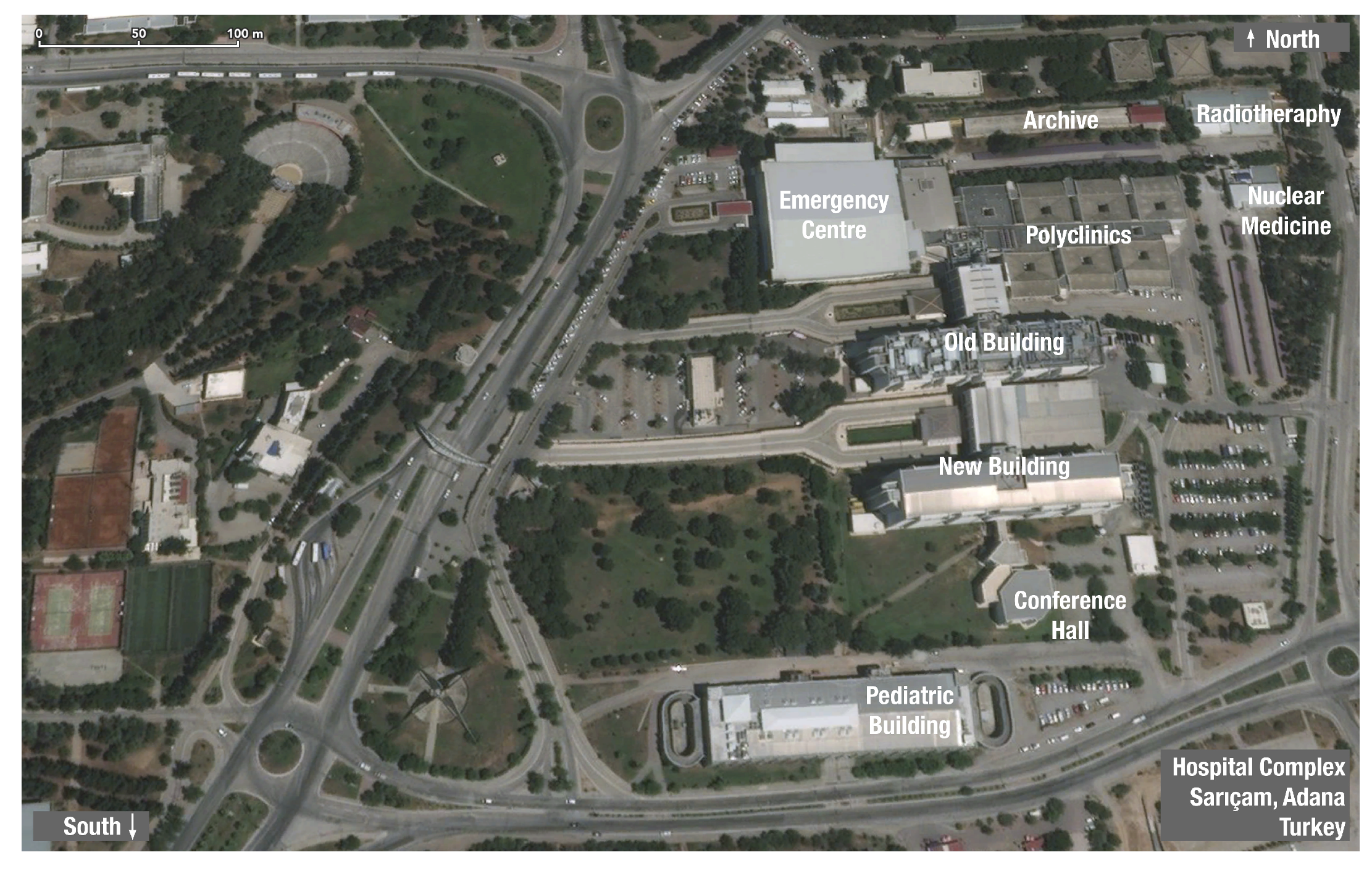
• An application of real-time short-term electrical energy consumption forecasting study with comprehensive meteorological observations is conducted for a large-scale hospital complex, including data acquisition, wrangling, and visualization in detail. Studies appertaining to short-term building electrical energy consumption forecasting is limited, especially for detailed real-time applications, and it is thought that this study will bridge the emphasized gap and strengthen the literature.
• Among various machine learning algorithms, GEP and GMDH networks are selected as forecasting methods for their capability of generating simple model equations between predictor variables and target variables without the necessity of performing feature selection. As far as is known, this study is the first attempt in the literature that compares GEP and GMDH networks for the prediction of short-term building electrical energy consumption. Both methods are implemented under identical constraints during a one-year period. Performing analyses with the same criteria reveals the genuine performance of each method for benchmarking purposes with respect to coefficient of determination (R${}^2$), root mean squared error (RMSE), and mean absolute percentage error (MAPE). For the first time, overall results of GEP and GMDH networks are interpreted from the points of accuracy, number of input parameters and complexity of model equations, and computational time. In addition to those, generated model equations in the context of this study can be employed for future studies regarding buildings having similar climatological conditions and electrical energy consumption profiles.
• To the best of one’s knowledge, an in-depth investigation of performance metrics acquired from the results of short-term building electrical energy consumption forecasting is firstly fulfilled in terms of several explanatory variables. Effects of short-wave irradiation, start and end of the shift hours, weekends and holidays, and seasonal transitions over short-term building electrical energy consumption forecasting are deduced along with hourly, daily, and monthly trends of prediction complexity in reference to MAPE.

The rest of the study is organized as follows: Section 2 presents the state-of-the-art review consisting of review studies intersecting building electrical energy consumption forecasting with artificial intelligence (AI), case studies in the field of short-term building electrical energy consumption prediction focusing on statistical and AI techniques for nonresidential buildings, and research studies utilizing GEP and GMDH networks for forecasting short-term electric load, demand, or electrical energy consumption; Section 3 introduces data source and acquisition, data wrangling, data set properties, and forecasting methods comprising the fundamentals of GEP and GMDH networks; Section 4 hosts discussion and experimental results of in-depth analyses; and finally, Section 5 concludes the study by emphasizing the prominent results for future studies.

2. Related Work

The literature contains a variety of successful reviews, which attempted to summarize building energy consumption forecasting methodologies from diverse perspectives. Firstly, Zhao and Magoules reviewed building energy consumption forecasting by classifying the methodologies, such as engineering methods, statistical methods, and AI methods [4]. Ahmad et al. summarized the applications of artificial neural networks (ANN) and support vector machines (SVM) for building energy consumption prediction by emphasizing the potential of a hybrid method that merges GMDH networks with least squares SVM (LSSVM) [5]. Raza and Khosravi conducted a review study on AI-based load demand forecasting techniques not only for buildings but also for smart grids by explaining all phases of short-term load forecasting comprehensively [6]. Daut et al. reviewed on the prediction of building electrical energy consumption by dividing the methodologies as conventional, AI, and hybrid methods [7]. Wang and Srinivasan compared single and ensemble models for AI-based building energy consumption forecasting within a review study [8]. Wei et al. presented a review of data-driven approaches for both prediction and classification of building energy consumption by mentioning practical applications of the approaches [9]. In a similar manner, Amasyali and El-Gohary reviewed data-driven building energy consumption forecasting studies by particularly focusing on the scopes of prediction, data properties and preprocessing methods, machine learning algorithms, and performance measures [10]. Lastly, Runge and Zmeureanu suggested a review for forecasting energy use in buildings utilizing ANN by highlighting applications, data, forecasting models, and performance metrics [11].

There are a limited number of studies in the literature that concentrated on short-term electrical energy consumption forecasting based on statistical and AI techniques for nonresidential buildings. Initially, Fan et al. presented a rigorous work about day-ahead building energy consumption forecasting, which employs an ensemble model in which weights are optimized by a genetic algorithm (GA), and the ensemble model consists of a single ANN, auto-regressive integrated moving average (ARIMA), boosting tree (BT), k-nearest neighbors (kNN), multivariate adaptive regression splines (MARS), multiple linear regression (MLR), random forests (RF), and support vector regression (SVR) [12]. Ke et al. analyzed the load profile and implemented hours-ahead building load forecasts by obtaining data from a substation feeder at the Centennial Campus of North Carolina State University and using similar day approach (SDA), direct curve fitting (DCF) with polynomial regression (PR), and MLR [13]. Wang et al. performed ensemble bagging trees (EBT) for forecasting hour-ahead energy consumption of Rinker Hall building in the University of Florida against a regression tree (RT) model [14]. Shabani and Zavalani utilized an incremental ANN approach against target mean (TM) for forecasting hour-ahead loads of a commercial building [15]. Zhu et al. compared performances of ANN by applying different strategies for neuron numbers, activation functions, data filtering, and regrouping for forecasting day-ahead loads acquired from two buildings in the City University of Hong Kong [16]. Yong et al. suggested implementing a combination of SDA and long-short term memory (LSTM) networks in comparison with ANN and a hybrid approach containing particle swarm optimization (PSO) and ANN for short-term load forecasting of a hotel building in Shanghai [17]. Ahmad et al. conducted a comprehensive work by obtaining data from a hotel building in Madrid and applied deep highway networks (DHN), SVR, and a tree-based ensemble (TBE) model for forecasting hour-ahead building heating, ventilation, and air-conditioning (HVAC) energy consumption [18]. Fang et al. tried to improve forecast accuracy by performing wavelet decomposition (WD) and ARIMA together as compared to the Holt-Winters method (HWM), LSTM, and seasonal auto-regressive integrated moving average (SARIMA) for daily energy consumption prediction of an office building in Qingdao, Shandong [19]. Fan et al. assessed deep network strategies including gated recurrent unit (GRU), LSTM, and recurrent neural networks (RNN) with several prediction approaches, such as direct, multi-input and multi-output (MIMO), and recursive approaches in order to forecast day-ahead energy consumption of an educational building in Hong Kong [20]. Finally, Divina et al. benchmarked different forecasting strategies, including ANN, ARIMA, ensemble, evolutionary algorithms (EA) for regression trees (EVTree), extreme gradient boosting (XGBoost), generalized boosted regression models (GBM), MLR, RF, and recursive partitioning and regression trees (RPart) for forecasting short-term electrical energy consumption of thirteen buildings belonging to a university campus in the south of Spain [21]. Comparative analysis of the aforementioned studies that processed short-term building electrical energy consumption forecasting is tabulated in

Table 1. Details of studies regarding short-term nonindustrial building electrical energy consumption forecasting.

	Performed	Building	Temporal	Forecast	Benchmark	Performance
	Model	Type	Granularity	Horizon	Models	Results
[12]	Ensemble	Skyscraper	15-min	Day-ahead	ANN & ARIMA &	2.320%
					BT & kNN &	(MAPE)
					MARS & MLR &
					RF & SVR
[13]	SDA	Campus	15-min	Hours-ahead	DCF-PR & MLR	2.170%
		Complex				(MAPE)
[14]	EBT	Campus	15-min	Hour-ahead	RT	3.170%
		Building				(MAPE)
[15]	ANN	Commercial	15-min	Hour-ahead	TM	N/A*
		Building
[16]	ANN	Campus	1-h	Day-ahead	ANN	4.969%
		Buildings				(MAPE)
[17]	SDA-LSTM	Hotel	30-min	Day-ahead	ANN & PSO-ANN	6.182%
		Building				(RE*)
[18]	DHN	Hotel	5-min	Hour-ahead	SVR & TBE	3.310 kWh
		Building				(RMSE)
[19]	WD-ARIMA	Office	1-h	Day-ahead	HWM & LSTM &	9.814%
		Building			SARIMA	(MAPE)
[20]	GRU	Educational	30-min	Day-ahead	LSTM & RNN	111.9 kWh
		Building				(RMSE)
[21]	RF	Campus	15-min	Day-ahead	ANN & ARIMA &	1.45 kW
		Buildings			Ensemble & EVTree &	(RMSE)
					XGBoost & GBM &
					MLR & RPart

* RE and N/A stand for relative error and not applicable.

, according to performed models, building type, temporal granularity of data set, forecast horizon, benchmark models, and performance results, respectively.

The literature comprises several studies that employed GEP and GMDH networks for short-term electrical energy consumption forecasting. Huo et al. developed an improved GEP model for short-term load forecasting and compared their model with traditional models of genetic programming (GP) and GEP [22]. Fan and Zhu indicated that a combination of empirical mode decomposition (EMD) and GEP may perform higher accuracy than WD and GEP combination for short-term load forecasting [23]. Hosseini and Gandomi compared GEP models with multiple least squares regression (MLSR) and generalized regression neural networks (GRNN) for forecasting day ahead peak and total loads of a North American electric utility [24]. Deng et al. used artificial fish swarm based hybrid GEP along with cloud computing in order to model distributed electric load forecasting in comparison with ANN, PSO-SVM, SVR, and traditional GEP on the data set of EUNITE competition [25].

Sforna used GMDH networks for acquiring a function between electric load and temperature variables and compared GMDH networks with ANN on electrical and meteorological data of four major Italian cities containing Florence, Milan, Naples, and Rome [26]. Huang and Shih utilized a combination of fuzzy modeling and GMDH networks on Taiwan’s electric load data in order to improve the performance of their short-term load forecast model against ANN and ARIMA [27]. Abdel-Aal employed GMDH networks on Seattle’s electrical and weather data to obtain analytical expressions between input and output variables in forecasting hourly and daily electric loads with different variations of ANN, abductive networks, and network committees (NC) [28,29,30]. Elattar et al. proposed a generalized locally weighted GMDH networks based EA for short-term load forecasting and performed the algorithm along with local support vector regression (LSVR), locally weighted GMDH networks (LWGMDH), locally weighted support vector regression (LWSVR), and traditional GMDH networks on two different data sets belonging to New York City and Victorian electricity market of Australia [31]. Xu et al. applied GMDH networks in comparison with ARIMA for short-term load forecasting of New South Wales in Australia [32]. Koo et al. presented a comparative study that performed ANN, simple exponential smoothing (SES), and GMDH networks for forecasting Korean electric load data on an hourly basis [33], and another study that wavelet transform was firstly applied for decomposition before the implementation of Holt-Winters method, ANN, and GMDH networks for one day ahead forecasting of hourly electric loads [34]. Jacob et al. employed GMDH networks and linear regression (LR) for forecasting short-term electrical energy consumption of a university campus in Nigeria [35]. Zjavka and Snasel proposed a method named as differential polynomial neural network that merges the functionality of GMDH networks with differential equation substitutions and carried out short-term load forecasting against ANN, SVM, and GMDH networks for the UK electricity transmission network and Canadian detached houses [36]. Yuniarti et al. tried to integrate wavelet transform with GMDH networks for short-term load forecasting of a power company in Sumatara, Indonesia, and collated it with the coefficient method (CM), which is currently used by the company [37]. Liu et al. enhanced GMDH networks by introducing elastic net regression and enriching with difference degree weighting optimization for forecasting hourly loads in data sets pertaining to three locations in China [38] against ANN, SVM, least absolute shrinkage and selection operator (LASSO), ridge regression (RR), and traditional GMDH networks. For South Korea’s hourly load data, Yu et al. suggested a forecasting methodology based on SVR, which implements GMDH networks and bootstrap methods for the input selection procedure in comparison with different variations of linear correlation (LC) and mutual information (MI) based filter methods [39]. Izzatillaev and Yusupov analyzed hourly electrical energy consumption forecasting in a grid-connected microgrid within a commercial bank by employing GMDH networks and ANN [40].

Benchmark analysis of the studies that utilized from GEP and GMDH networks for short-term electrical energy consumption forecasting is demonstrated in

Table 2. Details of studies employed gene expression programming (GEP) and group method of data handling (GMDH) networks for short-term electric load, demand, or electrical energy consumption forecasting.

	GEP	GMDH	Hybrid	Application	Forecast Horizon	Benchmark Models
[22]	•			Local Grid	Hour-ahead	GP & Traditional GEP
[23]	•		•	Local Grid	Hour-ahead	EMD-GEP & WD-GEP
[24]	•			National Grid	Day-ahead	GRNN & MLSR
[25]	•		•	National Grid	Day-ahead	ANN & PSO-SVM &
						SVR & Traditional GEP
[26]		•		National Grid	Day-ahead	ANN
[27]		•	•	National Grid	Day-ahead	ANN & ARIMA
[28]		•	•	National Grid	Hour-ahead &	ANN
					Day-ahead
[29]		•	•	National Grid	Day-ahead	ANN & NC
[30]		•	•	National Grid	Day-ahead &	ANN & Naïve Method
					Week-ahead
[31]		•		National Grid	Hour-ahead	LSVR & LWGMDH &
						LWSVR & Traditional GMDH
[32]		•		National Grid	Day-ahead	ARIMA
[33]		•		National Grid	Day-ahead	ANN & SES
[34]		•	•	National Grid	Day-ahead	ANN & Holt-Winters Method
[35]		•		Campus Complex	Day-ahead	LR
[36]		•	•	National Grid &	Day-ahead	ANN & SVM &
				Detached Houses		Traditional GMDH
[37]		•	•	National Grid	Day-ahead	CM
[38]		•	•	National Grid	Hour-ahead	ANN & LASSO-GMDH &
						RR-GMDH & SVM &
						Traditional GMDH
[39]		•	•	National Grid	Hour-ahead	LC & LC-GMDH &
						MI & MI-GMDH
[40]		•		Microgrid	Day-ahead	ANN

Local grid represents county level, while national grid corresponds to city level or larger.

in terms of performed models, application type, forecast horizon, and compared models, consecutively.

3. Material and Methods

As a general framework, this section is named as Material and Methods. Material of this study is the data set, and methods correspond to forecasting methods that can generate model equations for the prediction task.

3.1. Material

Material of the study is the data set, which is firstly acquired, then wrangled, and lastly prepared as electrical, meteorological, and calendar data. Steps are described as follows.

3.1.1. Data Source and Acquisition

Hospitals may be described as highly sophisticated organizations from the point of view of functional, technological, economic, managerial, and procedural aspects. The reliability of continuous energy flow has utmost importance for hospitals owing to their uninterrupted duty for 24/7 operation without any excuses. With its full name, Çukurova University Balcalı Health Application and Research Hospital is a large hospital complex and a pioneer health institution situated in Campus Balcalı of Çukurova University in Sarıçam district of Adana, Turkey. Since 1987, the hospital has been serving uninterruptedly to a region in the Southern Turkey by satisfying unceasing demands to supply electricity for an emergency service, 42 polyclinics, 12 intensive care units, 23 operating rooms, 43 clinical services, 5 laboratories, a radiology unit, a nuclear medicine, a blood center, a burn unit, a sterilization unit, and a pharmacy with also surgery rooms, laundries, kitchens, and a morgue [41]. The hospital has 1200 beds, serves more than 3500 patients per day with over 4000 academic and administrative staff, and has an installed transformer capacity around 18 MVA [42]. Aerial view of the hospital is illustrated in Figure 1.

Data acquisition stage covers an interval between 2 October 2017 and 1 October 2018 with a resolution of 10-min. Data acquisition terminal for the hospital is the medium-voltage switchgear building where the electricity meter of the hospital is located. Electrical data of the hospital were obtained from the hospital’s electricity meter via a three-phase energy logger during that interval. The logger is also in connection with an on-site temperature-humidity transducer that measure ambient temperature and relative humidity. The logger conducts logging by using the connections of current and voltage transformer in the terminal box of the electricity meter. Energy logger settings are adjusted to the multiplying factors of current and voltage transformers properly.

Other meteorological data were acquired from MERRA-2 (Modern-Era Retrospective Analysis for Research and Applications, Version 2), which is a database available worldwide of meteorological variables hosted by NASA and generated by the Goddard Space Flight Centre. The spatial resolution is approximately 50 km, which geographically corresponds to 0.625${}^{\circ }$ in latitude and 0.5${}^{\circ }$ in longitude [43]. The data acquisition stage is visualized in Figure 2.

3.1.2. Data Wrangling

Data wrangling can be stated as importing, tidying, and transforming data from its raw form to another format with an intention of making the data more valuable and suitable for sophisticated tasks.

Conversion of temporal granularity of the gathered data is accomplished from 10-min to 1-h via a forecast time horizon converter proposed in [42]. During the conversion process, missing values (a ratio of below 1% and occurred sporadically due to power outages at the hospital) and outliers are firstly detected and then treated via ARIMA with Kalman smoothing owing to its frequent use in recent energy studies [44,45] and superior performance in comparison with a variety of imputation methods employed in [42].

In brief, ARIMA with the Kalman smoothing imputation method performs Kalman smoothing on the state-space representation of an ARIMA model [46]. Analytically, Kalman filters are applied in two phases that are fundamentally based on the state-space models indicated in the following equations as

$$x_t=F_t{x}_{t-1}+{ϵ}_t$$

(1)

$$y_t=H_t{x}_t+{\omega }_t$$

(2)

where $x_t$ is the state vector of a given system at an instant in time t, $y_t$ is the reciprocating measurement vector at t, $F_t$ is the state-transition parameter of the system, ${ϵ}_t$ is the random state noise term, $H_t$ is the measurement parameter, and ${\omega }_t$ is the measurement error term. In the first phase, the state and the corresponding variance of the system is estimated by using Equation (1). In the second phase, the estimated phase is updated by performing both Equations (1) and (2). ARIMA with Kalman smoothing imputation method utilizes an automatic function that carries out a search in order to find the best ARIMA model [47].

After data wrangling, dimensionality of raw data possessing 52,416 rows and 19 columns is reduced by converting the raw data to a cleansed data set with 8736 rows and 18 columns representing input and target variables.

3.1.3. Data Set Properties

The data set employed for short-term building electrical energy consumption forecasting in this study has 3 input categories and 17 input variables that are summarised in

Table 3. Details of input variables.

Category	Symbol	Description	Unit	Minimum	Median	Mean	Maximum
Electrical	$E_h$	Previous 1 Hour	MWh	1.175	2.278	2.722	6.507
	$E_d$	Previous 1 Day (the same hour)	MWh	1.176	2.275	2.721	6.525
	$E_w$	Previous 1 Week (the same hour)	MWh	1.176	2.275	2.719	6.525
Meteorological	$T_D$	Transducer Device Temperature	${}^{\circ }$C	9.636	24.057	24.115	36.08
	$H_D$	Device Relative Humidity	%	15.0	52.56	50.67	75.9
	$T_O$	Outdoor Temperature	${}^{\circ }$C	1.534	20.856	21.148	42.175
	$H_O$	Outdoor Relative Humidity	%	6.377	60.813	58.73	100.0
	P	Pressure	hPa	963.1	984.4	984.8	1,002.6
	$W_S$	Wind Speed	m/s	0.075	2.463	2.798	11.648
	$W_D$	Wind Direction	${}^{\circ }$	0.263	171.003	146.529	359.617
	R	Rainfall	kg/m2	0.0	0.0002	0.065	7.994
	$I_{SW}$	Short-Wave Irradiation	Wh/m2	0.0	11.0	216.9	1024.2
Calendar	$h_{od}$	Hour of Day	–	0			23
	$d_{om}$	Day of Month	–	1			31
	$t_{od}$	Type of Day	–	0			1
	$w_{oy}$	Week of Year	–	1			53
	$m_{oy}$	Month of Year	–	1			12

.

Electrical variables standing for historical electrical energy consumption, meteorological variables taken from temperature–humidity transducer and MERRA-2, and calendar variables constitute the input variables of the data set.

Previous 1 h, 1 day, and 1 week electrical energy consumption values form retrospective electrical variables. Meteorological variables contain transducer device temperature and relative humidity, which are gathered from the on-site temperature–humidity transducer, and outdoor temperature and relative humidity, pressure, wind speed and direction, rainfall, and short-wave irradiation that are acquired from MERRA-2. Calendar variables are obtained from date and time logs of the energy logger and then evaluated as hour of day (0–23), day of month (1–31), type of day (0 for working days and 1 for weekends and public holidays), week of year (1–53), and month of year (1–12), respectively.

Actual electrical energy consumption, transducer device temperature, outdoor temperature, and short-wave irradiation graphs between October 2017 and October 2018 are illustrated in Figure 3.

3.2. Forecasting Methods

Fundamentals GEP and GMDH networks are, respectively, explained under the subsection of forecasting methods. Both methods can constitute analytical expressions for input variables and target variables without the need for the implementation of feature selection.

3.2.1. Gene Expression Programming

GEP is an enhanced methodology primarily based on GA and GP [48]. GEP contains five basic components, namely function set, terminal set, fitness function, control parameters, and termination condition.

Although parse tree demonstration is used in traditional GP, GEP employs a fixed length of character strings ([+, *, *, ${\beta }_1$, $x_1$, ${\beta }_2$, $x_2$] for the expression tree in Figure 4) for illustrating solutions to the problems, which are then visualized as parse trees [24]. The illustration of trees in GEP is named as expression tree and shown in Figure 4. The expression tree shown in Figure 4 corresponds to Equation (3).

$$y={\beta }_1{x}_1+{\beta }_2{x}_2$$

(3)

The flowchart of the GEP algorithm is indicated in Figure 5. Shortly, the mechanism starts with random production of chromosomes to generate the first population. Afterwards, expression of chromosomes and evaluation of each individual’s fitness are carried out consecutively. Next, the selection of individuals are implemented with respect to fitness for reproduction with modification. The process is repeated for a determined number of productions or up to a solution [48].

In other words, mathematical evolution initially starts with producing candidate functions, followed by mutation, breeding, and lastly, natural selection in order to model the data as close as possible. In addition to functions and variables, expression can possess constants. The constants can evolve by assignation of the values explicitly or randomly. For the optimization of random constants, nonlinear regression algorithms, such as differential evolution, Gauss-Newton, Levenberg–Marquardt, or a combination of them, can be employed for refining the constants. Advantages and disadvantages of GEP are described in

Table 4. Advantages and disadvantages of GEP.

Advantages	Disadvantages
1. Extremely versatile	1. Does not ensure that the levels of functional complexity in the phenotype are also directly reflected in the genotype
2. Easy to understand with its linear and ramified structure	2. The best individual is maintained, but some of better individuals may be lost
3. Faster than old GAs	3. Needs much additional computation owing to mutations, crossovers, and rotations before reaching an optimal solution
4. Has no invalid individuals	4. Indicates premature convergence
5. Overcomes the shortcomings of GA and GP

.

Among GEP applications, symbolic regression is a broadly utilized method to obtain an analytical expression for a desired output from input variables of a given data set. Each sample of the data set contains input variables and outputs, which can be stated as

$$\{x_{i,1},x_{i,2},\dots ,x_{i,n},o_{i,1},\dots ,o_{i,m}\}$$

where n represents the number of input variables, and m corresponds to the number of outputs, $x_{i,j}$ and $o_{i,j}$ are the jth input and output of the ith sample. MSE or RMSE is frequently used for the accuracy of fitting. The symbolic regression needs to find the optimal ${\Gamma }^{*}$ that minimizes the error for the given data set

$${\Gamma }^{*}={arg}_{\Gamma }minf(\Gamma )$$

where $\Gamma$ is the quality of the formula, $f(\Gamma )$ gives the fitting error of $\Gamma$ [49].

3.2.2. GMDH Networks

GMDH networks, namely polynomial neural networks, principally operate as self-organizing networks where neuron connections, number of selected neurons, layers, and neurons in hidden layers are not constant and are self-acting along with training in order to reach an optimal model for maximum accuracy without overfitting [50]. To do so, GMDH networks use least squares regression to find the best mathematical relation among input and output variables by a reference function, which can be expressed as

$$y=a_0+\sum _{i=1}^n{a}_i{x}_i+\sum _{i=1}^n\sum _{j=1}^n{a}_{ij}{x}_i{x}_j+\sum _{i=1}^n\sum _{j=1}^n\sum _{k=1}^n{a}_{ijk}{x}_i{x}_j{x}_k+\dots$$

(4)

where y corresponds to the output, $X=(x_1,x_2,\dots ,x_n)$ represents the input vector, and a symbolizes either the coefficient or weight vector [51].

Ordinarily, the previous equation is utilized in the quadratic form of two variables such that

$$y=a_0+a_1{x}_i+a_2{x}_j+a_3{x}_i{x}_j+a_4{x}_i^2+a_5{x}_j^2$$

(5)

In GMDH networks, input layer contains neurons for each input variable indicated by x as illustrated in Figure 6. Each neuron in the first layer acquires its inputs from two of the neurons in the input layer. The neurons in the second and the third layers obtain their inputs from two of the neurons in the previous layer and this process continues up to output layer. The output layer takes two of its inputs from the previous layer and generates the final result that shows the most suitable analytical expression in satisfying the relationship between input and output variables. The flowchart of GMDH networks is indicated in Figure 7 [52].

If n is the number of neurons in a layer in GMDH networks, then the number of candidate neurons in the next layer will be calculated as

$$\left(\genfrac{}{}{0pt}{}{n}{2}\right)=\frac{n\times (n-1)}{2}$$

(6)

for two variable polynomials. Additionally, it should be noted that one neuron also may skip layers directly from the input variables to one of the next layers in GMDH networks as demonstrated with dashed lines from $x_5$ to $z_6$ in Figure 6 as an example.

During the training process, two different sets of input data are employed, namely main training data and control data, which is used for overfitting. The control data generally contain about 20% as many rows as the main training data. During the training algorithm, MSE is computed for each neuron and also applied to the control data. If the MSE of the best neuron in the current layer as measured with the control data is lower than the MSE of the best neuron in the previous layer, and the maximum number of layers has not yet been obtained, the training process continues to construct the next layer. Otherwise, the training process halts. It should be noted that when overfitting starts, the error as measured with the control data will increase, therefore the training process will stop.

Pros and cons of GMDH networks are stated in

Table 5. Pros and cons of GMDH networks [53,54].

Pros	Cons
1. Presents adaptive network topologies which can be customized to the given problem	1. Tends to produce quite complex polynomials for simple systems
2. Finds locally good weights owing to the reliability of the fitting technique	2. Do not guarantee building up the true structure
3. Can be trained rapidly by sparse connectivity	3. Biased estimates of coefficients due to the least squares method

.

4. Results and Discussion

All computations in the scope of this work were performed on a Macintosh computer with OS version of 10.15.2, a processor of 2.4 GHz (Intel Core i5), and a memory size of 8 GB. For all computing tasks, RStudio was used as an integrated development environment for R programming language, which is one of the most popular languages for statistical computing and data analytics with elegant graphics [55].

Values stored in input variables of the data set are scaled between 0 and 1 for normalization, which provides elimination of units of various data types, reducing computational time and covering less memory for data integrity, and benchmarking multiple data columns in a similar way. In the assessment of performances belonging to GEP and GMDH networks, R², RMSE, and MAPE are utilized in this study. Formulae of the performance metrics are as follows:

$$R^2=1-\frac{{\sum }_{i=1}^n{(y_i-{\widehat{y}}_i)}^2}{{\sum }_{i=1}^n{(y_i-\overline{y})}^2}$$

$$RMSE=\sqrt{\frac{{\sum }_{i=1}^n{(y_i-{\widehat{y}}_i)}^2}{n}}$$

$$MAPE(\%)=\frac{100}{n}\sum _{i=1}^n\frac{|y_i-{\widehat{y}}_i|}{|y_i|}$$

where $y_i$ is actual or measured output, $\widehat{y}$ is predicted output, $\overline{y}$ is mean of $y_i$, and n indicates the number of observations [41].

For model testing and evaluation, random sampling method is implemented to GEP and GMDH networks in such a manner that 20% of the data set is employed to constitute training data, and 80% of the data set is adopted to form validation data randomly.

4.1. Parameters of GEP

Model building parameters for GEP are used as 50 for population size, 10,000 for the number of maximum tries for initial population, 4 for genes of chromosome, 8 for gene head length, 2000 for number of maximum generations, 1000 for number of generations without improvement, and 1.0 for the best chromosome’s fitness score stop. Fitness properties are determined as MSE for fitness function, 1% for hit tolerance, and 100 for selection range. During computations, allowed functions are addition (+), subtraction (−), multiplication (×), division (/), and square root ($\sqrt{\phantom{25}}$), while algebraic simplifications are conditionally permitted. The rates of evolution parameters are specified as 4.4% for mutation, 10% for gene, inversion, insertion sequence transposition, root insertion sequence transposition, and gene transposition, and 30% for both one-point and two-point. Addition (+) is employed as the link function for all genes. Features of random constants are adjusted as 10 for random real constants per gene, −10 and 10 for minimum and maximum constant values, and 1% for mutation rate.

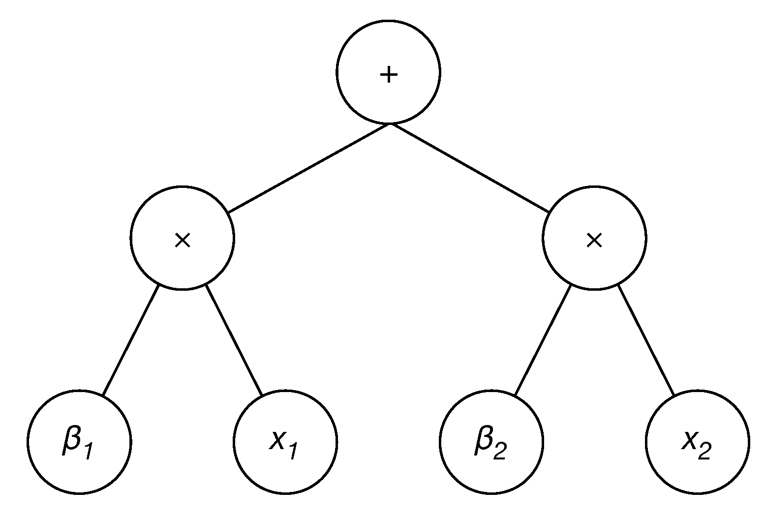
Generations required for the training model and simplification are 2001 and 407, respectively. The complexity of the model is reduced from 25 to 15 by simplification. Evaluations of fitness function are numbered as 125,150. The best GEP model containing four input variables is demonstrated in Figure 8 and yields the following equation

$$\widehat{E}=\frac{2I_{SW}}{h_{od}-1.068}+E_h-0.367T_O-2.726$$

where $\widehat{E}$ is the predicted electrical energy consumption, $T_O$ and $I_{SW}$ represent the outdoor temperature and short-wave irradiation values taken from MERRA-2, $E_h$ corresponds to the electrical energy consumption value for the previous one hour, and $h_{od}$ is the value of calendar variable standing for hour of day.

4.2. Parameters of GMDH Networks

For GMDH networks, the quadratic reference function with two variables stated in Equation (5) is employed. Parameters for the GMDH networks are predetermined as 20 for the number of both maximum network layers and neurons per layer, 16 for maximum polynomial order, and ${10}^{-4}$ for convergence tolerance. Allowed network configuration for the neurons in the next layer is designated as the selection of neurons in the previous layer and original input variables. A hold-out sample of 20% is utilized for protection control in order to avoid overfitting.

The best GMDH network model having seven input variables is found as

$$\widehat{E}=0.616+0.079N_1+0.920N_{11}+0.140N_1{N}_{11}-0.007N_1^2-0.007N_{11}^2$$

(7)

where N corresponds to neurons from $N_1$ to $N_{16}$ such that each neuron represents a quadratic equation, $T_D$ and $H_D$ stand for transducer device temperature and relative humidity, $t_{od}$ symbolizes the calendar variable type of day, and $E_d$ indicates the electrical energy consumption for the previous day at the same hour. Detailed parameters and coefficients of Equation (7) are given in

Table 6. Parameters and coefficients of the best GMDH network model.

Equation Parameters and Coefficients
$\mathit{y}$	${\mathit{x}}_{\mathit{i}}$	${\mathit{x}}_{\mathit{j}}$	${\mathit{a}}_{\mathbf{0}}$	${\mathit{a}}_{\mathbf{1}}$	${\mathit{a}}_{\mathbf{2}}$	${\mathit{a}}_{\mathbf{3}}$	${\mathit{a}}_{\mathbf{4}}$	${\mathit{a}}_{\mathbf{5}}$
$N_3$	$H_D$	$E_h$	2720.12	8.181	1260.335	7.878	2.440	0.707
$N_6$	$I_{SW}$	$E_h$	2728.9	18.633	1256.047	8.301	−5.258	−4.619
$N_2$	$N_3$	$N_6$	−1.383	0.116	0.885	0.007	−0.004	−0.004
$N_9$	$T_D$	$E_h$	2729.678	−11.248	1271.363	1.325	−6.409	−2.147
$N_8$	$N_9$	$N_6$	−1.248	−0.306	1.307	0.023	−0.012	−0.012
$N_1$	$N_2$	$N_8$	4.022	−0.745	1.742	0.209	−0.104	−0.104
$N_{13}$	$t_{od}$	$E_d$	1.682 × 1013	1.357 × 1013	1242.167	−84.608	−1.682 × 1013	−56.185
$N_{12}$	$N_{13}$	$N_6$	0.535	0.004	0.996	10−5	−5 × 10−6	−4 × 10−6
$N_{16}$	$h_{od}$	$N_6$	−6.061	−2.276	1	10−4	4.218	4.727 × 10−8
$N_{11}$	$N_{12}$	$N_{16}$	12.577	0.783	0.211	0.602	−0.301	−0.301
$\widehat{E}$	$N_1$	$N_{11}$	0.616	0.079	0.920	0.140	-0.007	-0.007

.

4.3. Overall Results

Correlation coefficients of input, target, and predictor variables are visualized as a map in Figure 9 according to Pearson’s correlation prior to mentioning overall results. Pearson’s correlation indicates a number between −1 and 1 that shows the extent to which two variables are linearly correlated. It should be emphasized that blank squares within the correlation map represent statistically insignificant p-values that are smaller than 0.01.

When overall performances of the applied methods are evaluated in terms of accuracy, it is seen that GMDH networks give slightly better results than GEP according to R², RMSE, and MAPE for the short-term building electrical energy consumption forecasting problem, as shown in

Table 7. Overall performances of the applied methods.

	GMDH				GEP
	R2	RMSE	MAPE	Run Time	R2	RMSE	MAPE	Run Time
Performance	(%)	(kWh)	(%)	(s)	(%)	(kWh)	(%)	(s)
Overall	99.960	25.067	0.620	585.9	99.955	26.668	0.641	145.5

.

However, it should be noted that the best GMDH network model employs seven input variables with different variations in several equations having high polynomial order, while the best GEP model executes four input variables in one simple equation. Therefore, the simplicity of the GEP model reveals the fact that the computational time required to reach the best model by using GEP is one fourth of the time needed for GMDH networks, as indicated in Figure 10.

Thus, the selection of each method for short-term building electrical energy consumption forecasting problem depends on the order of importance. If accuracy is more important than computational time and simpleness, GMDH networks are recommended. Otherwise, GEP is suggested for its low computational complexity and run time.

Additionally, graphs consisting of actual and predicted values by employing GEP and GMDH networks are demonstrated in Figure 11 for 9–10 October 2017 and 23–24 April 2018, which are the days possessing the largest errors because of seasonal transitions (from summer to winter and from winter to summer).

4.4. Discussion of In-Depth Investigation Results

Daylight utilization is one of the crucial topics not only for electrical energy efficiency studies but also for architectural indoor lighting studies. Short-wave irradiation is active during daylight and considered as a prominent variable that affects energy consumption of sustainable buildings. One distinctive finding of this study is related to the effect of short-wave irradiation over short-term building electrical energy consumption forecasting. $I_{SW}$ is encountered in both model equations; hence, it draws the attention and is advised to be included as an explanatory variable for further studies. Short-wave irradiation affects outdoor and indoor temperature, which also have impacts on the building HVAC temperature set point that influences electrical energy consumption. This study unveils that if short-wave irradiation does not equal zero, the arduousness level of short-term building electrical energy consumption prediction significantly increases, as indicated in

Table 8. The effect of short-wave irradiation over short-term building electrical energy consumption forecasting.

	GMDH			GEP
	R2	RMSE	MAPE	R2	RMSE	MAPE
Feature	(%)	(kWh)	(%)	(%)	(kWh)	(%)
$I_{SW}=0$	99.974	17.240	0.505	99.970	18.608	0.512
$I_{SW}\ne 0$	99.949	30.101	0.717	99.943	31.895	0.749

.

Another innovative result of this work, which has never processed in the literature to the best of one’s knowledge, are in-depth investigations of the error-related performance metrics regarding short-term forecasts with respect to hour of day, name of day, type of day, and name of month. Short-term forecasts are examined according to the hour of day, in order to deduce the challenging hours in building electrical energy consumption prediction. It is inferred from the obtained results presented in

Table 9. In-depth investigation of short-term forecasts in reference to the hour of day.

	GMDH			GEP
	R2	RMSE	MAPE	R2	RMSE	MAPE
Hour of Day	(%)	(kWh)	(%)	(%)	(kWh)	(%)
00:00–01:00	99.984	13.225	0.483	99.986	12.438	0.361
01:00–02:00	99.988	11.223	0.360	99.987	11.580	0.372
02:00–03:00	99.988	10.646	0.353	99.988	10.638	0.376
03:00–04:00	99.987	10.922	0.371	99.983	12.598	0.428
04:00–05:00	99.971	16.409	0.525	99.961	18.926	0.690
05:00–06:00	99.951	21.275	0.582	99.943	22.990	0.717
06:00–07:00	99.874	35.268	1.169	99.868	36.194	1.197
07:00–08:00	99.697	62.834	1.844	99.670	65.609	1.889
08:00–09:00	99.944	30.380	0.725	99.928	34.600	0.823
09:00–10:00	99.964	25.543	0.608	99.968	24.361	0.639
10:00–11:00	99.970	24.105	0.584	99.977	21.254	0.557
11:00–12:00	99.976	22.029	0.535	99.982	18.831	0.476
12:00–13:00	99.968	25.394	0.615	99.981	19.330	0.477
13:00–14:00	99.978	21.665	0.475	99.977	22.392	0.468
14:00–15:00	99.980	20.714	0.529	99.982	19.852	0.466
15:00–16:00	99.971	24.806	0.561	99.960	29.044	0.662
16:00–17:00	99.892	43.816	1.269	99.814	57.393	1.464
17:00–18:00	99.972	20.180	0.573	99.959	24.485	0.652
18:00–19:00	99.977	17.292	0.467	99.969	20.080	0.512
19:00–20:00	99.974	17.822	0.513	99.978	16.407	0.535
20:00–21:00	99.979	15.894	0.411	99.983	14.174	0.425
21:00–22:00	99.985	13.257	0.370	99.986	13.104	0.388
22:00–23:00	99.982	14.300	0.416	99.985	13.168	0.409
23:00–24:00	99.978	15.996	0.549	99.984	13.624	0.404

that two hours and an hour before the shift start (06:00–07:00 and 07:00–08:00) have the largest errors and are difficult to predict along with the previous hour of the shift end (16:00–17:00). The forecasts in terms of the name of day are analyzed in detail and the results are shared in

Table 10. In-depth investigation of short-term forecasts with respect to the name of day.

	GMDH			GEP
	R2	RMSE	MAPE	R2	RMSE	MAPE
Day of Week	(%)	(kWh)	(%)	(%)	(kWh)	(%)
Monday	99.950	29.600	0.727	99.945	31.088	0.709
Tuesday	99.955	27.718	0.659	99.946	30.386	0.700
Wednesday	99.959	26.898	0.643	99.951	29.301	0.674
Thursday	99.954	27.348	0.652	99.948	29.146	0.670
Friday	99.957	26.541	0.649	99.949	28.873	0.677
Saturday	99.974	17.484	0.516	99.976	16.943	0.527
Sunday	99.976	16.505	0.496	99.977	16.124	0.531

. In regard to Table 10, the complexity level of prediction shows a tendency to decrease from the first day of the week (Monday) to the end of the week (Sunday). In the forecasts according to the type of day, in-depth analyses indicate that forecasting working days are more difficult than predicting weekends and holidays, as illustrated in

Table 11. In-depth investigation of short-term forecasts according to the type of day.

	GMDH			GEP
	R2	RMSE	MAPE	R2	RMSE	MAPE
Type of Day	(%)	(kWh)	(%)	(%)	(kWh)	(%)
Working Days	99.954	27.929	0.673	99.945	30.188	0.697
Weekends & Holidays	99.976	17.186	0.504	99.978	16.489	0.519

.

Months with peak errors are elaborated in

Table 12. In-depth investigation of short-term forecasts in terms of the name of month.

		GMDH			GEP
		R2	RMSE	MAPE	R2	RMSE	MAPE
Year	Month	(%)	(kWh)	(%)	(%)	(kWh)	(%)
2017	October	99.721	26.667	0.779	99.714	26.980	0.774
	November	99.753	16.927	0.646	99.736	17.513	0.678
	December	99.751	17.676	0.617	99.729	18.431	0.647
2018	January	99.743	19.981	0.643	99.721	20.812	0.659
	February	99.750	16.993	0.591	99.737	17.457	0.619
	March	99.763	13.863	0.574	99.752	14.164	0.619
	April	99.781	20.757	0.769	99.781	20.762	0.795
	May	99.898	24.090	0.628	99.892	24.849	0.648
	June	99.788	31.506	0.596	99.768	32.928	0.610
	uly	99.821	32.761	0.523	99.778	36.534	0.542
	August	99.811	31.906	0.489	99.770	35.193	0.492
	September	99.822	35.193	0.593	99.785	38.625	0.617

wherein October and April possess the largest errors in comparison with the others owing to the fact that in the mentioned months, significant meteorological changes occur due to seasonal transitions from summer to winter and vice versa.

Key results of the in-depth investigations are summarized in Figure 12. Effect of shift start and end on an hourly basis, decreasing trend from Monday to Sunday, and peak errors of months during seasonal transitions are highlighted in Figure 12 with respect to GEP and GMDH networks.

5. Conclusions

Share of buildings energy consumption in the global final energy use and evolution of existing electric power systems to smart grids and IoE are considered together, the significance of short-term building electrical energy consumption forecasting is comprehended. Complexity of the forecasting process comes from the fact that there are so many factors influencing building energy consumption and every building has its own characteristics, such as physical properties and operational schedule.

Recent studies in the literature show an interest in the application of machine learning algorithms to predict short-term building electrical energy consumption. However, most of them produce an abstruse analytical expression among explanatory variables and response variables. In this study, GEP and GMDH networks are employed to forecast short-term building electrical energy consumption for a large hospital complex in the Eastern Mediterranean owing to their capability of generating easily understandable model equations between input variables and target variables without the need of implementing feature selection. Both methods are performed under identical constraints and evaluated in terms of R², RMSE, and MAPE.

According to the results of the analyses, the best MAPE scores of GMDH networks and GEP are calculated as 0.620% and 0.641%, respectively. It is considered that GEP can be chosen for its low computational complexity and run time, while GMDH networks may be selected for predictions holding slightly better accuracy. In-depth investigations are carried out in this study to generalize and highlight the increase in forecasting complexity during challenging transitional periods by investigating MAPE values. Acquired results deduce the effects of short-wave irradiation, start and end of the working hours, weekends and holidays, and seasonal transitions over short-term building electrical energy consumption forecasting along with hourly, daily, and monthly trends of the prediction arduousness with respect to MAPE.

Consequently, it should be emphasized that this study is the first attempt in the literature that benchmarks GEP and GMDH networks for short-term building electrical energy consumption forecasting to create genuine and simple model equations by interpreting remarkable results with regards to accuracy, number of input parameters and complexity of model equations, and computational time. Furthermore, produced model equations in this study can be utilized for future studies related to buildings possessing similar meteorological conditions and electrical energy consumption profiles.

References

1. The International Energy Agency. 2019 Global Status Report for Buildings and Construction: Towards a Zero-Emissions, Efficient and Resilient Buildings and Construction Sector; Technical Report; The International Energy Agency: Paris, France, 2019. [Google Scholar]
2. Hong, T.; Fan, S. Probabilistic electric load forecasting: A tutorial review. Int. J. Forecast. 2016, 32, 914–938. [Google Scholar] [CrossRef]
3. Zor, K.; Timur, O.; Teke, A. A state-of-the-art review of artificial intelligence techniques for short-term electric load forecasting. In Proceedings of the 2017 6th International Youth Conference on Energy (IYCE), Budapest, Hungary, 21–24 June 2017; pp. 1–7. [Google Scholar] [CrossRef]
4. Zhao, H.; Magoules, F. A review on the prediction of building energy consumption. Renew. Sustain. Energy Rev. 2012, 16, 3586–3592. [Google Scholar] [CrossRef]
5. Ahmad, A.; Hassan, M.; Abdullah, M.; Rahman, H.; Hussin, F.; Abdullah, H.; Saidur, R. A review on applications of ANN and SVM for building electrical energy consumption forecasting. Renew. Sustain. Energy Rev. 2014, 33, 102–109. [Google Scholar] [CrossRef]
6. Raza, M.Q.; Khosravi, A. A review on artificial intelligence based load demand forecasting techniques for smart grid and buildings. Renew. Sustain. Energy Rev. 2015, 50, 1352–1372. [Google Scholar] [CrossRef]
7. Daut, M.A.M.; Hassan, M.Y.; Abdullah, H.; Rahman, H.A.; Abdullah, M.P.; Hussin, F. Building electrical energy consumption forecasting analysis using conventional and artificial intelligence methods: A review. Renew. Sustain. Energy Rev. 2017, 70, 1108–1118. [Google Scholar] [CrossRef]
8. Wang, Z.; Srinivasan, R.S. A review of artificial intelligence based building energy use prediction: Contrasting the capabilities of single and ensemble prediction models. Renew. Sustain. Energy Rev. 2017, 75, 796–808. [Google Scholar] [CrossRef]
9. Wei, Y.; Zhang, X.; Shi, Y.; Xia, L.; Pan, S.; Wu, J.; Han, M.; Zhao, X. A review of data-driven approaches for prediction and classification of building energy consumption. Renew. Sustain. Energy Rev. 2018, 82, 1027–1047. [Google Scholar] [CrossRef]
10. Amasyali, K.; El-Gohary, N.M. A review of data-driven building energy consumption prediction studies. Renew. Sustain. Energy Rev. 2018, 81, 1192–1205. [Google Scholar] [CrossRef]
11. Runge, J.; Zmeureanu, R. Forecasting Energy Use in Buildings Using Artificial Neural Networks: A Review. Energies 2019, 12. [Google Scholar] [CrossRef] [Green Version]
12. Fan, C.; Xiao, F.; Wang, S. Development of prediction models for next-day building energy consumption and peak power demand using data mining techniques. Appl. Energy 2014, 127, 1–10. [Google Scholar] [CrossRef]
13. Ke, X.; Jiang, A.; Lu, N. Load profile analysis and short-term building load forecast for a university campus. In Proceedings of the 2016 IEEE Power and Energy Society General Meeting (PESGM), Boston, MA, USA, 17–21 July 2016; pp. 1–5. [Google Scholar] [CrossRef]
14. Wang, Z.; Srinivasan, R.; Wang, Y. Homogeneous Ensemble Model for Building Energy Prediction: A Case Study Using Ensemble Regression Tree. In Proceedings of the 2016 ACEEE Summer Study on Energy Efficiency in Buildings, Pacific Grove, CA, USA, 21–26 August 2016; pp. 1–12. [Google Scholar]
15. Shabani, A.; Zavalani, O. Hourly Prediction of Building Energy Consumption: An Incremental ANN Approach. Eur. J. Eng. Res. Sci. 2017, 2, 27–32. [Google Scholar] [CrossRef] [Green Version]
16. Zhu, G.; Chow, T.T.; Tse, N. Short-term load forecasting coupled with weather profile generation methodology. Build. Serv. Eng. Res. Technol. 2018, 39, 310–327. [Google Scholar] [CrossRef]
17. Yong, Z.; Xiu, Y.; Chen, F.; Pengfei, C.; Binchao, C.; Taijie, L. Short-term building load forecasting based on similar day selection and LSTM network. In Proceedings of the 2018 2nd IEEE Conference on Energy Internet and Energy System Integration (EI2), Beijing, China, 20–22 October 2018; pp. 1–5. [Google Scholar] [CrossRef]
18. Ahmad, M.W.; Mouraud, A.; Rezgui, Y.; Mourshed, M. Deep Highway Networks and Tree-Based Ensemble for Predicting Short-Term Building Energy Consumption. Energies 2018, 11. [Google Scholar] [CrossRef] [Green Version]
19. Fang, C.; Gao, Y.; Ruan, Y. Improving forecasting accuracy of daily energy consumption of office building using time series analysis based on wavelet transform decomposition. IOP Conf. Ser. Earth Environ. Sci. 2019, 294, 012031. [Google Scholar] [CrossRef] [Green Version]
20. Fan, C.; Wang, J.; Gang, W.; Li, S. Assessment of deep recurrent neural network-based strategies for short-term building energy predictions. Appl. Energy 2019, 236, 700–710. [Google Scholar] [CrossRef]
21. Divina, F.; García Torres, M.; Gomez Vela, F.A.; Vazquez Noguera, J.L. A Comparative Study of Time Series Forecasting Methods for Short Term Electric Energy Consumption Prediction in Smart Buildings. Energies 2019, 12. [Google Scholar] [CrossRef] [Green Version]
22. Huo, L.; Yin, J.; Guo, L.; Hu, J.; Fan, X. Short-Term Load Forecasting Based on Improved Gene Expression Programming. In Proceedings of the 2008 4th IEEE International Conference on Circuits and Systems for Communications, Shanghai, China, 26–28 May 2008; pp. 745–749. [Google Scholar] [CrossRef]
23. Fan, X.; Zhu, Y. The application of Empirical Mode Decomposition and Gene Expression Programming to short-term load forecasting. In Proceedings of the 2010 Sixth International Conference on Natural Computation, Yantai, China, 10–12 August 2010; Volume 8, pp. 4331–4334. [Google Scholar] [CrossRef]
24. Sadat Hosseini, S.S.; Gandomi, A.H. Short-term load forecasting of power systems by gene expression programming. Neural Comput. Appl. 2012, 21, 377–389. [Google Scholar] [CrossRef]
25. Deng, S.; Yuan, C.; Yang, L.; Zhang, L. Distributed electricity load forecasting model mining based on hybrid gene expression programming and cloud computing. Pattern Recognit. Lett. 2018, 109, 72–80. [Google Scholar] [CrossRef]
26. Sforna, M. Searching for the electric load-weather temperature function by using the group method of data handling. Electr. Power Syst. Res. 1995, 32, 1–9. [Google Scholar] [CrossRef]
27. Huang, S.J.; Shih, K.R. Application of a fuzzy model for short-term load forecast with group method of data handling enhancement. Int. J. Electr. Power Energy Syst. 2002, 24, 631–638. [Google Scholar] [CrossRef]
28. Abdel-Aal, R.E. Short-term hourly load forecasting using abductive networks. IEEE Trans. Power Syst. 2004, 19, 164–173. [Google Scholar] [CrossRef]
29. Abdel-Aal, R. Improving electric load forecasts using network committees. Electr. Power Syst. Res. 2005, 74, 83–94. [Google Scholar] [CrossRef]
30. Abdel-Aal, R. Modeling and forecasting electric daily peak loads using abductive networks. Int. J. Electr. Power Energy Syst. 2006, 28, 133–141. [Google Scholar] [CrossRef]
31. Elattar, E.E.; Goulermas, J.Y.; Wu, Q.H. Generalized Locally Weighted GMDH for Short Term Load Forecasting. IEEE Trans. Syst. Man Cybern. Part C (Appl. Rev.) 2012, 42, 345–356. [Google Scholar] [CrossRef]
32. Xu, H.; Dong, Y.; Wu, J.; Zhao, W. Application of GMDH to Short-Term Load Forecasting. In Advances in Intelligent Systems; Lee, G., Ed.; Springer: Berlin/Heidelberg, Germany, 2012; pp. 27–32. [Google Scholar]
33. Koo, B.; Lee, S.; Kim, W.; Park, J.H. Comparative Study of Short-Term Electric Load Forecasting. In Proceedings of the 2014 5th International Conference on Intelligent Systems, Modelling and Simulation, Langkawi, Malaysia, 27–29 January 2014; pp. 463–467. [Google Scholar] [CrossRef]
34. Koo, B.G.; Lee, H.S.; Park, J. Short-term Electric Load Forecasting Based on Wavelet Transform and GMDH. J. Electr. Eng. Technol. 2015, 10, 832–837. [Google Scholar] [CrossRef] [Green Version]
35. Jacob, T.; Usman, U.A.; Bemdoo, S.; Susan, A.A. Short-term Electrical Energy Consumption Forecasting Using GMDH-type Neural Network. J. Electr. Electron. Eng. 2015, 3, 42–47. [Google Scholar] [CrossRef] [Green Version]
36. Zjavka, L.; Snasel, V. Short-term power load forecasting with ordinary differential equation substitutions of polynomial networks. Electr. Power Syst. Res. 2016, 137, 113–123. [Google Scholar] [CrossRef]
37. Yuniarti, T.; Surjandari, I.; Muslim, E.; Laoh, E. Data mining approach for short term load forecasting by combining wavelet transform and group method of data handling (WGMDH). In Proceedings of the 2017 3rd International Conference on Science in Information Technology (ICSITech), Bandung, Indonesia, 25–26 October 2017; pp. 53–58. [Google Scholar] [CrossRef]
38. Liu, W.; Dou, Z.; Wang, W.; Liu, Y.; Zou, H.; Zhang, B.; Hou, S. Short-Term Load Forecasting Based on Elastic Net Improved GMDH and Difference Degree Weighting Optimization. Appl. Sci. 2018, 8. [Google Scholar] [CrossRef] [Green Version]
39. Yu, J.; Park, J.H.; Kim, S. A New Input Selection Algorithm Using the Group Method of Data Handling and Bootstrap Method for Support Vector Regression Based Hourly Load Forecasting. Energies 2018, 11. [Google Scholar] [CrossRef] [Green Version]
40. Izzatillaev, J.; Yusupov, Z. Short-term Load Forecasting in Grid-connected Microgrid. In Proceedings of the 2019 7th International Istanbul Smart Grids and Cities Congress and Fair (ICSG), Istanbul, Turkey, 25–26 April 2019; pp. 71–75. [Google Scholar] [CrossRef]
41. Timur, O.; Zor, K.; Çelik, Ö.; Teke, A.; İbrikçi, T. Application of Statistical and Artificial Intelligence Techniques for Medium-Term Electrical Energy Forecasting: A Case Study for a Regional Hospital. J. Sustain. Dev. Energy Water Environ. Syst. 2019, 1–17. [Google Scholar] [CrossRef] [Green Version]
42. Zor, K. Research and Application of Real-Time Short-Term Electrical Energy Consumption Forecasting Using Artificial Intelligence Based Techniques. Ph.D. Thesis, Çukurova University, Institute of Natural and Applied Sciences, Adana, Turkey, 2019. [Google Scholar]
43. Gelaro, R.; McCarty, W.; Suárez, M.J.; Todling, R.; Molod, A.; Takacs, L.; Randles, C.A.; Darmenov, A.; Bosilovich, M.G.; Reichle, R.; et al. The Modern-Era Retrospective Analysis for Research and Applications, Version 2 (MERRA-2). J. Clim. 2017, 30, 5419–5454. [Google Scholar] [CrossRef] [PubMed]
44. Yang, J.; Tan, K.K.; Santamouris, M.; Lee, S.E. Building Energy Consumption Raw Data Forecasting Using Data Cleaning and Deep Recurrent Neural Networks. Buildings 2019, 9. [Google Scholar] [CrossRef] [Green Version]
45. Demirhan, H.; Renwick, Z. Missing value imputation for short to mid-term horizontal solar irradiance data. Appl. Energy 2018, 225, 998–1012. [Google Scholar] [CrossRef]
46. Moritz, S.; Bartz-Beielstein, T. imputeTS: Time Series Missing Value Imputation in R. R J. 2017, 9, 207. [Google Scholar] [CrossRef] [Green Version]
47. Hyndman, R.J.; Khandakar, Y. Automatic Time Series Forecasting: TheforecastPackage forR. J. Stat. Softw. 2008, 27. [Google Scholar] [CrossRef] [Green Version]
48. Ferreira, C. Gene Expression Programming: A New Adaptive Algorithm for Solving Problems. Complex Syst. 2001, 13, 87–129. [Google Scholar]
49. Zhong, J.; Feng, L.; Ong, Y.S. Gene Expression Programming: A Survey [Review Article]. IEEE Comput. Intell. Mag. 2017, 12, 54–72. [Google Scholar] [CrossRef]
50. Giorgi, M.D.; Malvoni, M.; Congedo, P. Comparison of strategies for multi-step ahead photovoltaic power forecasting models based on hybrid group method of data handling networks and least square support vector machine. Energy 2016, 107, 360–373. [Google Scholar] [CrossRef]
51. Xiao, J.; Li, Y.; Xie, L.; Liu, D.; Huang, J. A hybrid model based on selective ensemble for energy consumption forecasting in China. Energy 2018, 159, 534–546. [Google Scholar] [CrossRef]
52. Dag, O.; Yozgatligil, C. GMDH: An R Package for Short Term Forecasting via GMDH-Type Neural Network Algorithms. R J. 2016, 8, 379–386. [Google Scholar] [CrossRef] [Green Version]
53. Onwubolu, G. GMDH-Methodology and Implementation in C; Imperial College Press: Singapore, 2015. [Google Scholar]
54. Stepashko, V.; Bulgakova, O.; Zosimov, V. Construction and Research of the Generalized Iterative GMDH Algorithm with Active Neurons. In Advances in Intelligent Systems and Computing II; Shakhovska, N., Stepashko, V., Eds.; Springer: Cham, Switzerland, 2018; pp. 492–510. [Google Scholar]
55. R Core Team. R: A Language and Environment for Statistical Computing; R Foundation for Statistical Computing: Vienna, Austria, 2019. [Google Scholar]
Figure 1. Aerial view of the hospital complex.
Energies 13 01102 g001
Figure 2. Visualization of data acquisition stage.
Energies 13 01102 g002
Figure 3. Illustration of actual electrical energy consumption, transducer device and outdoor temperature, and short-wave irradiation between logging period.
Energies 13 01102 g003
Figure 4. Demonstration of an expression tree.
Energies 13 01102 g004
Figure 5. The flowchart of GEP algorithm.
Energies 13 01102 g005
Figure 6. An illustration of GMDH networks.
Energies 13 01102 g006
Figure 7. The flowchart of GMDH networks.
Energies 13 01102 g007
Figure 8. Expression tree of the best GEP model.
Energies 13 01102 g008
Figure 9. Correlation map of input, target, and predicted variables.
Energies 13 01102 g009
Figure 10. Illustration of computational time and polynomial order of GEP and GMDH networks.
Energies 13 01102 g010
Figure 11. Demonstration of actual and predicted samples during transition seasons.
Energies 13 01102 g011
Figure 12. Illustration of the results of in-depth analyses.
Energies 13 01102 g012