Test and Modeling of the Hydraulic Performance of High-Efficiency Cooling Configurations for Gyrotron Resonance Cavities

Abstract

The design and manufacturing of different full-size mock-ups of the resonance cavity of gyrotrons, relevant for fusion applications, were performed according to two different cooling strategies. The first one relies on mini-channels, which are very promising in the direction of increasing the heat transfer in the heavily loaded cavity, but which could face an excessively large pressure drop, while the second one adopts the solution of Raschig rings, already successfully used in European operating gyrotrons. The mock-ups, manufactured with conventional techniques, were hydraulically characterized at the Thales premises, using water at room temperature. The measured pressure drop data were used to validate the corresponding numerical computational fluid dynamics (CFD) models, developed with the commercial software STAR-CCM+ (Siemens PLM Software, Plano TX, U.S.A.) and resulting in excellent agreement with the test results. When the validated models were used to compare the two optimized cooling configurations, it resulted that, for the same water flow, the mini-channel strategy gave a pressure drop was two-fold greater than that of the Raschig rings strategy, allowing a maximum flow rate of 1 × 10⁻³ m³/s to meet a maximum allowable pressure drop of 0.5 MPa.

1. Introduction

Electron cyclotron resonance heating (ECRH) is one of the three plasma heating devices used in nuclear fusion machines [1] based on the magnetic confinement of plasma, with examples such as tokamaks [2] and stellarators [3]. The ECRH relies on high-power generators operating in the MW range at millimetric wave frequencies for continuous wave pulses, for which gyrotron oscillators [4] are widely employed as a consolidated solution. In a gyrotron, sketched in Figure 1a, a large energy transfer between an annular rotating beam and a fast wave occurs in the little volume of the waveguide, which behaves as a true open-ended resonant cavity (see Figure 1b), and it is affected by important power dissipations on the surfaces where a critically high heat load needs to be managed. As a result, the gyrotron performances depend crucially on the heat sink capability and thermomechanical stability of the resonant cavity. An efficient cooling allows selecting, between higher-order operative modes, those with higher beam/wave interaction efficiency [5]. With the right compromise, even if higher power dissipation can occur, a larger portion of the beam will interact successfully with the electromagnetic radiation, resulting in a global increase of the radio frequency (RF) output power generation for the same direct current (DC) beam power. A higher power extracted from the beam results in a greater electromagnetic field in the cavity, resulting in higher induced current on the cavity walls and consequent Joule heating to be managed.

The actual cooling systems of the W7-X and the International Thermonuclear Experimental Reactor (ITER) European Gyrotrons [6], [7], namely, Thales TH1507 and Thales TH1509, respectively, are based on the Thales patented Raschig rings (RRs) technology [8], a well-known technological solution adopted originally as column packing in distillation and then in packed beds, especially for chemical processes [9]. A Raschig’s ring (RR), named after its inventor, is a small hollow cylinder (with the same length and height) made from copper, coated with a metal alloy. Several rings are packed in the thin annulus constituting the cavity, in which the electromagnetic interaction occurs, and brazed together thanks to the coating, resulting in a porous structure with high thermal conductivity. The RR technology in the cavity resonator was already proven to be capable of managing heat load peaks up to ~20 MW/m², but its suitability to bear the even higher heat fluxes, foreseen for the European Union (EU) DEMOnstration power plant gyrotron [7], is under investigation, in view of the uncertainties in its removal capability.

In order to improve the heat management of cavities, targeted to the design of higher-RF-efficiency tubes, several alternative options are being investigated, such as axial or longitudinal grooves [10] or mini-channels (MC) [11,12,13,14]. The MC cooling option was tested in a planar cavity mock-up at the Areva premises [13], in conditions relevant for the cavity operation [15]. The results were encouraging, and the MC was adopted in the design of the cavity under development at Karlsruher Institut für Technologie (KIT) for a high-power gyrotron [16]. That option, consisting of a series of circular or semi-circular channels drilled all around the cavity, exploits a high-speed turbulent flow for the coolant and, thus, large heat transfer coefficient, overcoming the RR limitations in terms of low water-flow velocity. If, on the one hand, the MC option can overcome the RR option in terms of heat removal capability (thermal performance), then, on the other hand, the large flow section available for the coolant in the RR configuration (which is the reason for the above-mentioned low water-flow velocity) potentially ensures, with respect to the MC option, a reduced pressure drop (hydraulic performance).

However, no direct comparison between the two options, whether in terms of hydraulic or thermal performance, was done so far. Here, we concentrate on the first aspect, i.e., the hydraulic performance, and we establish the first direct comparison between the MCs and RRs when used in the same cavity, by testing and modeling the hydraulic characteristics of the two different configurations.

After a technological investigation to verify the feasibility of the mini-channels by additive manufacturing, a full-size cavity mock-up was manufactured with standard techniques (see Section 2), and it was tested at the Thales premises in Velizy-Villacoublay to measure the hydraulic characteristic. The experimental results were compared to those obtained from a full-size cavity mock-up equipped with Raschig rings, as reported in Section 3.

In parallel, an effort was performed to develop computational fluid dynamics (CFD) models which could help in designing future optimized cavities. The numerical model of the RR solution was built here using the discrete element model (DEM) CFD approach [17], as already successfully done, for instance, in Reference [18] for a fixed-bed reactor where RRs were used as a porous matrix, or in Reference [19]. That approach, which allows discrete pellet CFD simulations of flow field and pressure drop accounting for all the different rings, randomly filling the computational domain, is applied here in a completely different context than the chemical field. The alternative approach for the modeling of the RRs, namely, rigid body dynamics (RBD) CFD [20,21], although very useful for the hydraulic (and thermal) simulations, was not considered here since it is not available in the commercial software STAR-CCM+, which we selected for the CFD analysis. The development of the model for the fluid flow in the mock-up equipped with MC does not pose particular challenges from the computational point of view, since a similar model was already validated against the experimental data coming from the test of the planar mock-up, as shown in Reference [15].

The models and their validation against the experimental data are reported in Section 4, where the main features of the numerical results are also discussed. In Section 5, a comparison between the hydraulic performance of the two optimized cooling configurations is performed.

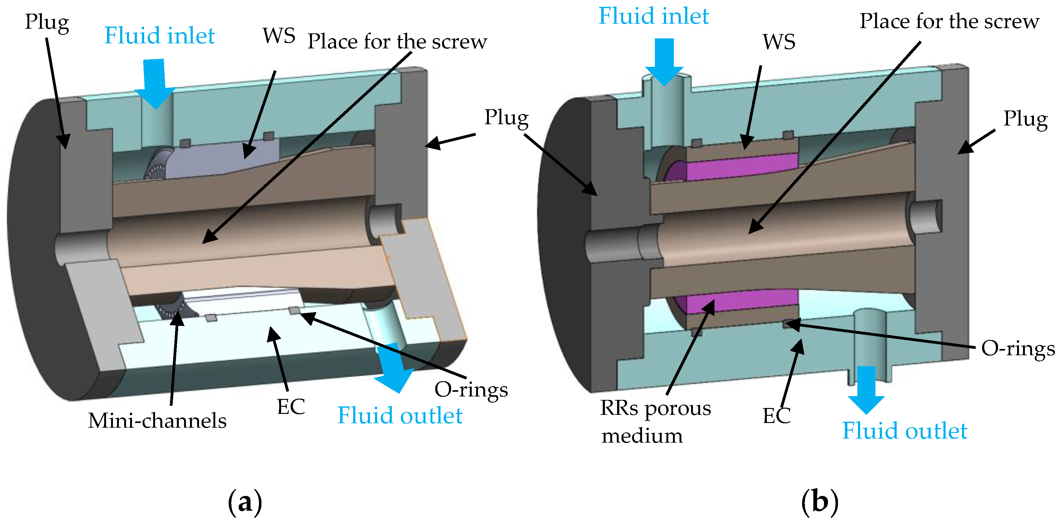
2. The Cavity Mock-Ups

All the mock-ups constituted the following components: resonant cavity, water-stopper (WS), external cylinder (EC), two plugs, one screw, and two hydraulic connectors; however, they differed in view of the cooling strategy: mini-channels (Figure 2a) or Raschig rings (Figure 2b). Due to the different materials used to realize the mock-ups, some geometrical details of the cooling chambers were adjusted while assuring that the introduced differences were negligible from the point of view of the hydrodynamic behavior.

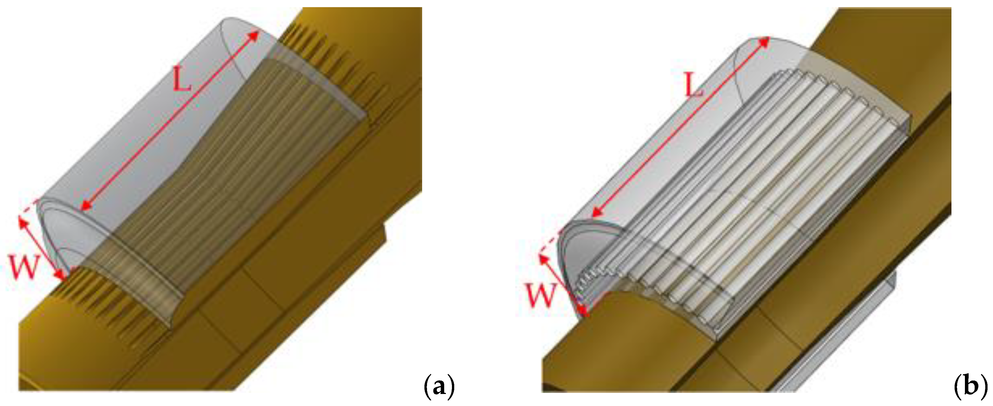
2.1. Mock-Ups Equipped with Mini-Channels

Two different mock-ups, with axial extension of 100 mm, were realized keeping the same external envelope, but using different cavities, both equipped with mini-channels (Figure 2a and Figure 3, respectively).

In the first mock-up, both the resonator and the water-stopper were realized in a single piece of CuC₂ (pure additive copper), because of the complex shape of the MCs, using an additive technology ideated by Thales (see Figure 3a), in the frame of additive manufacturing. The MCs, with a cross-section composed of a semicircle merged to a rectangle, resulting in a total flow section of ~1 mm² (see zoomed-in image in Figure 3a), were displaced all around the cavity with a pitch of ~2.5 mm, and they were designed to axially follow the external axial profile of the cavity, resulting in a bend along their length (configuration A), as shown in Figure 4a. The chosen MC shape and path were the result of an optimization study carried out in Reference [22], which involved thermo-mechanical and electro-dynamic aspects, in addition to thermal–hydraulic aspects. Since the choice of the additive technology was also aimed at investigating the maturity of this technology, some preliminary checks and analyses were performed on the manufactured cavity. A tomographic analysis revealed the presence of some materials inside the channels, with some channels completely plugged at least in one location (see Figure 5). A permeability test confirmed the porosity of the material, which was expected to some extent. The technology was then considered to be not yet mature for this kind of application. For this reason, a second mock-up, again equipped with MCs, was realized with traditional machining methods, in order to carry out the hydraulic measurements.

In the second mock-up (see Figure 3b) the resonator and water-stopper were made using a lathe machine in a single piece of nylon. The MCs were realized using a high-precision drilling machine. Because of the use of traditional machining methods, the MCs had a more conventional circular section, with a diameter of ~2 mm and a pitch of ~3 mm. They did not follow the profile of the external wall of the cavity (Figure 3b), resulting axially straight (configuration B), as shown in Figure 4b.

The EC was made of Plexiglass, and its internal radius was slightly larger than the external one of the water-stopper in order to allow the insertion of the cavity. Two O-rings were inserted into two slots drilled into the Plexiglass, according to the WS position, in order to lock the cavity in the mock-up and prevent the water from going into the empty space between the WS and the EC, as shown in Figure 2a. Two cylindrical holes were realized in the EC, where two hydraulic connectors were inserted, to insert the mock-up in the test loop used for the hydraulic measurements.

Two aluminum plugs were realized to hold the cylinder, and they were tightly connected by a screw which traversed the entire mock-up (see Figure 2), in order to ensure that no water could flow inside the inner volume, which was smaller than that of the true resonant cavity for the nylon MC mock-up.

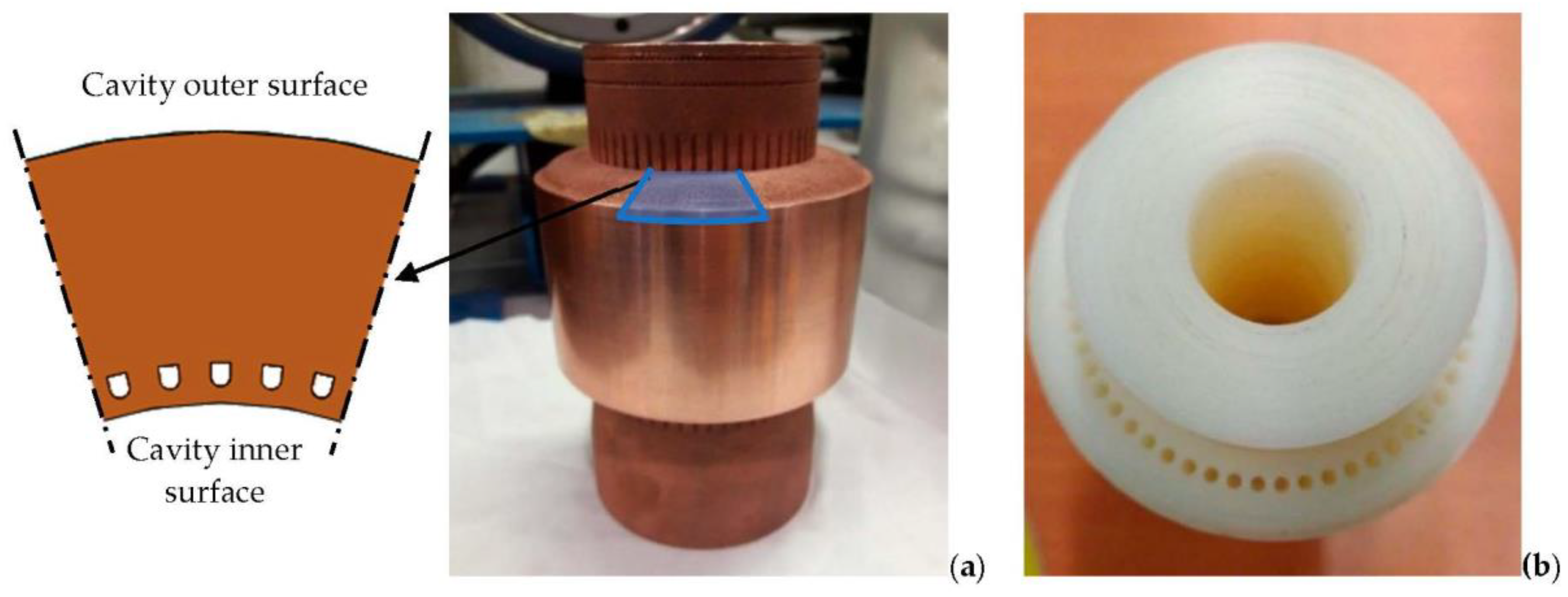
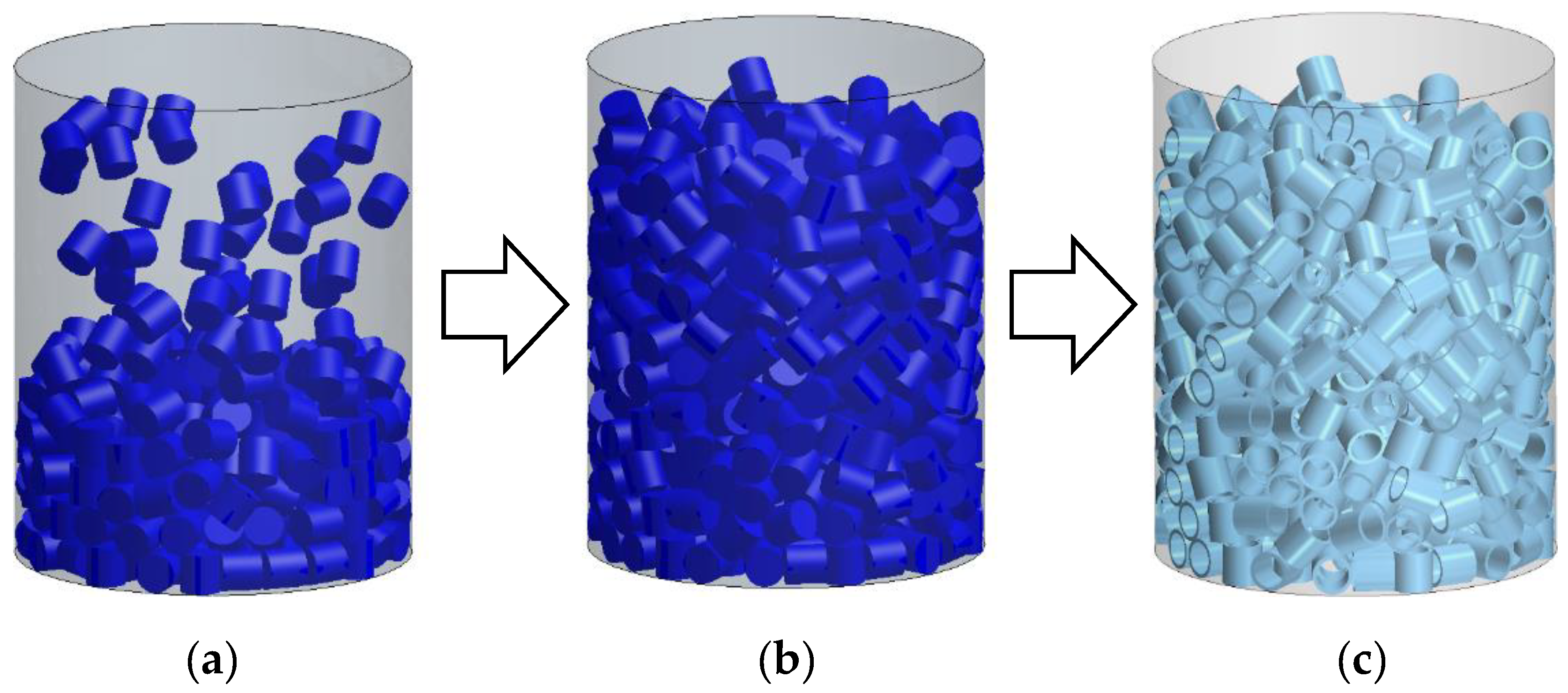
2.2. Mock-Up Equipped with RRs

In the RR mock-up, the cooling system consisted of a porous medium made up of a certain number of small hollow cylinders forming a macaroni-like structure (Figure 6a). The cylinders were made of copper and their dimensions, length, and diameter were on the order of millimeters.

In order to produce the porous medium (Figure 6b), the RRs, coated with a thin layer of a brazing alloy, were injected into the region between the resonator and the WS, and then they were brazed in a furnace following a Thales reserved process. Note that, in the manufactured mock-up, the radial extension of the RR region was reduced with respect to the current gyrotron design, in order to drive a higher water speed and eventually a higher heat transfer coefficient in the cavity. The idea of reducing the radial extension of the RR region and plugging the rest of the available space with a WS, as shown in Figure 2b, was based on the numerical observation that only the first few layers of rings contributed actively to the cooling of the cavity in operation [8].

The external cylinder and the plugs used for the RR mock-up were identical to those used for the MC mock-up (Figure 2b).

3. Test Set-Up and Results

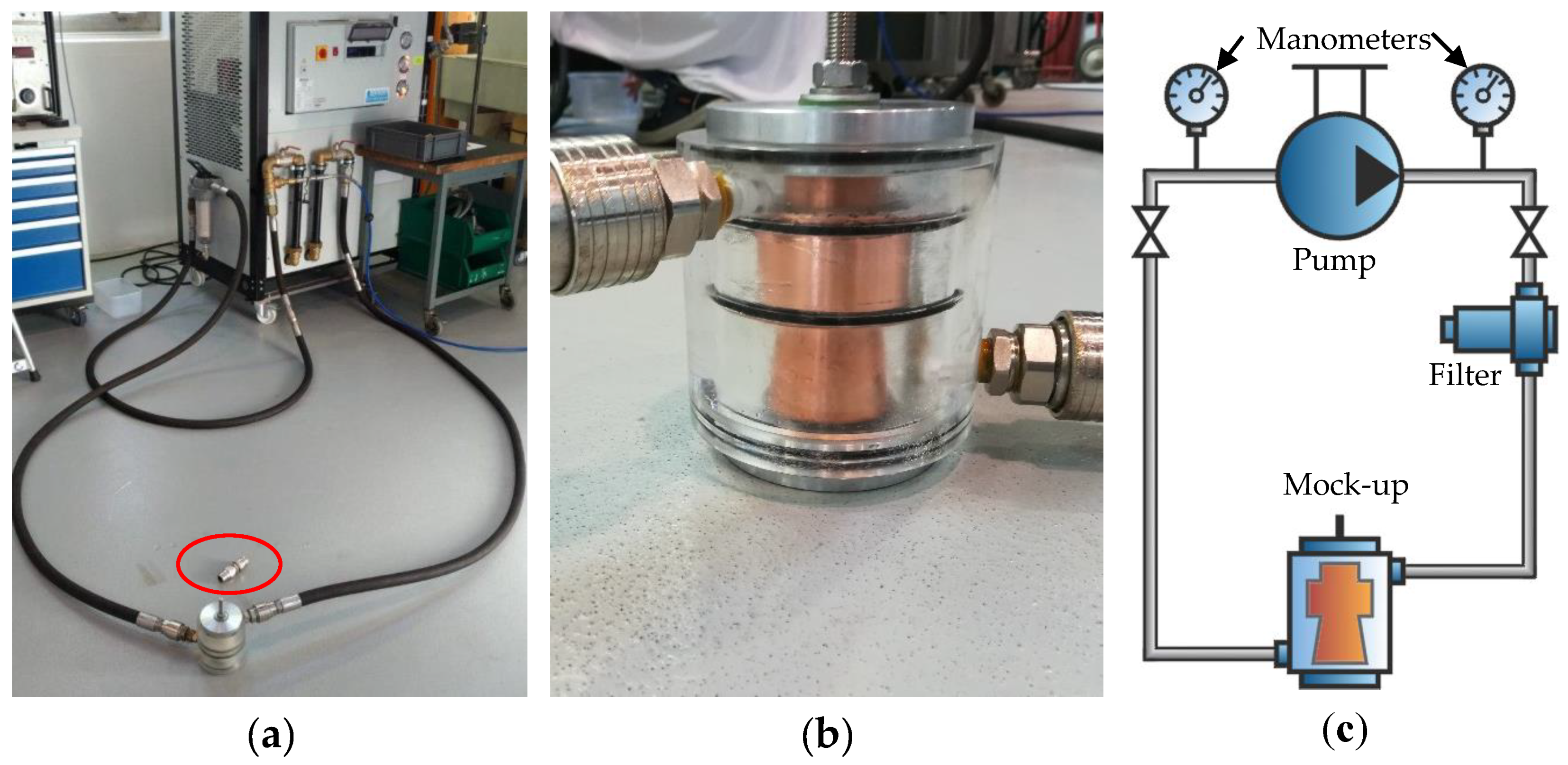
3.1. Test Facility

To perform the hydraulic tests and measure the hydraulic characteristics of the two cavity cooling options, a small water test loop already present in Thales was used (Figure 7a). The very simple loop consisted of a pump and of two pipes at its outlet and inlet (inlet and outlet of the mock-up, respectively, Figure 7b), equipped with two manometers, measuring the fluid pressure at outlet ($p_{out,pump}$) and inlet ($p_{inlet,pump}=p_{outlet,mock-up}$) of the pump, respectively. A filter for the water was added before the mock-up inlet (Figure 7c), to avoid the circulation of impurities. The variable-speed pump allowed choosing the water flow rate (reported in L/min, and converted in the paper to m³/s for convenience), and the tests for both mock-ups were performed varying the flow rate from 10 L/min to 80 L/min (from 0.17 × 10⁻³ to 1.3 × 10⁻³ m³/s, respectively) The pressure head given by the pump, which was equal to the pressure drop along the loop including the mock-up, named, $\Delta p_{mock-up+loop},$ could be evaluated as the difference between outlet and inlet pressure, as shown in Equation (1).

$$\Delta p_{mock-up+loop}=p_{out,pump}-p_{inlet,pump}.$$

(1)

A calibration of the pressure drop across the entire loop was performed in order to take into account (1) the pressure drops of the loop not directly related to the cavity, i.e., those related to the loop piping, (2) the filter, and (3) the hydraulic adapters used to connect the loop pipes to the mock-ups. For the calibration, the hydraulic adapters were directly linked by a short hydraulic connector, the pressure loss of which could be neglected. The pressure drop of the entire loop excluding the mock-up, named $\Delta p_{loop}$, was equal to the pressure head of the pump, and it could be then computed similarly to Equation (1) by using the manometer measurements in the flow rate range 0.17 × 10⁻³ m³/s to 1.3 × 10⁻³ m³/s.

The mock-up pressure drop at the different flow rates, named $\Delta p_{mock-up}$, was then evaluated, at any flow rate value, as the difference between the $\Delta p_{mock-up+loop}$ and $\Delta p_{loop}$, as reported in Equation (2).

$$\Delta p_{mock-up}=\Delta p_{mock-up+loop}-\Delta p_{loop}.$$

(2)

Concerning the precision of the values given by the machine, the following factors were taken into consideration:

-

The precision on the flow rate was equal to ±1 L/min (±0.17 × 10⁻⁴ m³/s).

-

Any pressure value was measured with a precision of ±0.1 bar. Since the pressure drop could be evaluated here just as the difference between two pressure values, measured by independent manometers, the uncertainty of pressure drop doubled due to error propagation. The final pressure drop $\Delta p_{mock-up}$ was, in turn, the difference between two pressure drops (see Equation (2)), based on the readouts of the same two manometers (see Equation (1)). Their errors could not be considered independent; thus, we conservatively kept the uncertainty on $\Delta p_{mock-up}$ frozen to ±0.2 bar. Note that the experimental facility was originally configured to test components with a much higher pressure drop than those of the two mock-ups, so that the use of a differential pressure sensor, which would help in reducing the uncertainty, was not considered.

3.2. Test Results for the Mini-Channel Mock-Up

Hydraulic tests with water at room temperature were performed using both copper and nylon cavity mock-ups. In the copper case, the measured pressure drops were far higher than the expected values. This can be explained considering the presence of some channels being plugged, as seen with the tomography (see Figure 5). For this reason, the results could not be compared with simulations, and they are not reported. This also led to the conclusion that, as mentioned before, the additive technology adopted is not mature enough to be used for the manufacturing of gyrotron cavities.

The results of the nylon mock-up test are reported in Figure 8a, and they can be compared to those in Figure 8b, where the results obtained during the tests of the RR mock-up are reported. In those images, the results of the dedicated calibration tests, which were performed again, are included, confirming those already shown in Figure 8a. The same results, more conveniently represented in terms of pressure drop, with or without mock-ups, are reported in Figure 9a,b. While the loop pressure drop is shown to be very well reproducible, the pressure drop with the two mock-ups was significantly different, showing a ~20–25% lower drop at 8.33 × 10⁻⁴ m³/s (operating condition of the ITER gyrotron) for the straight MCs, with respect to the RR configuration. However, the straight MC configuration was not fully relevant for the gyrotron cooling, and it was developed for ease of manufacturing, aimed at the numerical model validation (see Section 4).

4. Simulations

A hydraulic numerical analysis was carried out on the mock-ups equipped with RRs and MCs using the commercial software STAR-CCM+ through a three-dimensional, steady-state model, solving the Navier–Stokes equations [23].

The computational domain was restricted in both cases to just the fluid domain inside the mock-up, including the water inlet and outlet, since we limit the analysis here to the pure hydraulic characteristic of the component.

4.1. The DEM for the Raschig Rings

While the simulation of the fluid flow inside the circular pipes presented no difficulties at all (see below), the simulation of the flow inside the RR region was a challenge, which could be overcome by adopting the DEM tool available in the selected software, as done in previous works on the same topic [8].

The RR matrix generation procedure consisted of three steps. In the first step, the volume of the RR matrix was created (see Figure 2b). The second step was the actual DEM simulation, consisting of a time-dependent study in which, at each time step (0.01 s), a certain number of cylindrical particles, of the same outer size of the RR, were injected into the volume where the porous matrix should be built (the cylinder, for instance, in Figure 10a). During the simulation, the particles fell in the direction of gravity and accumulated at the bottom, forming a porous matrix. The procedure of the particle injection stopped when the number of cylinders reached the value needed to achieve the target porosity of 78.8% (based on the nominal value for the gyrotron cavities manufactured by Thales (Figure 6b). Note, however, that the value, based on previous experience, could be affected by an uncertainty of ~±2%. The result of the DEM simulation at that stage was a compact matrix of solid cylinders (Figure 10b). In the last step of the procedure, the solid cylinders were replaced by the hollow cylinders, which had the same outer dimension (Figure 10c).

4.2. Turbulence Model

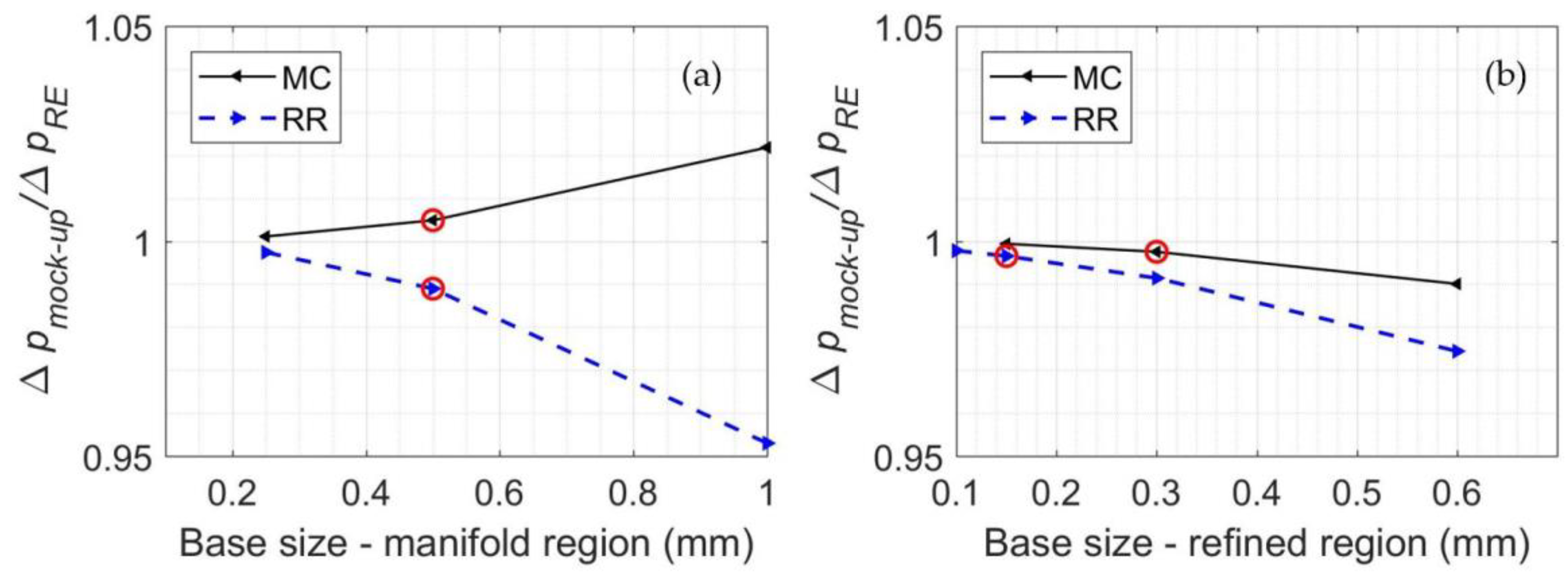
The flow was in turbulent conditions for all the simulated values of the flow rates, which varied in the simulations from 5.0 × 10⁻⁴ to ~1.2 × 10⁻³ m³/s. At the pipe inlet and outlet, the value of the Reynolds number Re was between 60,000 and 150,000. The turbulent conditions in the RR region were evaluated looking at the “pellet Reynolds number” Re_p, defined using the mean velocity at the inlet of the RR region and the characteristic length computed as the diameter of the sphere equivalent to the volume of a single ring. Turbulent conditions are achieved when Re_p > 600 [21], and, in the case at hand, we computed values between 1700 and 5000. In the MC region, Re (defined using the pipe diameter as characteristic length) varied from 7000 to 18,000; thus, the flow was confirmed to be in the turbulent regime.

A two-equation Reynolds-averaged Navier–Stokes (RANS) k–ω SST [24] model was chosen in the simulations for both mock-ups, with an all-y+ wall treatment. The Reynolds-averaged Navier–Stokes (RANS) equations describe the behavior of a turbulent flow with a time-averaging approach; thus, each instantaneous quantity is split into its time-averaged and fluctuating components [25]. In particular, a k–ω model has improved performance in modeling the boundary layers under adverse pressure gradients, which is a critical feature of the cases under study. The chosen model SST-Menter k–ω works as a standard k–ω in the near-wall region, and as a k–ε model in the fully turbulent region [26]. Note that, in Reference [21], the realizable k–ε model with an enhanced wall treatment (EWT) was preferred, based on the fact that, for the application presented there, it was a “tried-and-tested RANS model” for simulating flow fields with strong streamline curvature. To demonstrate the suitability of the SST-Menter k–ω model for the application we present here, a comparison simulation with the k–ε model was carried out (see below).

4.3. Grid

For both mock-ups, hybrid grids were adopted, made up of polyhedral elements in the bulk regions and a prismatic layer near the walls. In order to choose the proper size of cells, a grid independence study was conducted, considering only a piece of the entire circular fluid domain, corresponding to an angle of 20°, as shown in Figure 11. The rationale behind the grid generation was to use two different base sizes: a fine grid in the MC/RR regions and a coarse grid in the rest of the computational domain. At first, a refinement of the cell base size of the fluid region in the inlet/outlet manifold (i.e., excluding the RRs and MCs portion of the domain) was done. Once the optimum size was chosen, finding a compromise between the solution precision and the computational cost of the simulations, a study of the cell base size in the refined region of the RRs and MCs was performed. As a last step, the number of prism layers was varied (three, five, 10); in all cases, the mesh layers near the wall were built in order to keep $y^{+}~1$, so that the same mesh could be eventually used for accurate thermal simulations.

A selection of the grid independence analysis results is shown in Figure 12 in terms of the pressure drop computed across the mock-ups, normalized to the asymptotic solution evaluated through a Richardson extrapolation [27]. It is shown that the selected grid parameters allowed computing the pressure drop with a small deviation (within ~1%) from that of the Richardson extrapolation for both models. The final grid, the parameters of which are collected in

Table 1. Topological details of the computational grids developed for the MC and RR models.

Model	Base Size in Manifold Region (mm)	Bas Size in the Refined Region (mm)	Number of Prism Layers	Total Number of Cells (Million)
MCs	0.5	0.3	5	17.7
RRs	0.5	0.15	5	25.4

, had smaller elements in the regions of major interest, such as in the MC and RR regions, as shown in the insets in Figure 13 and Figure 14, respectively.

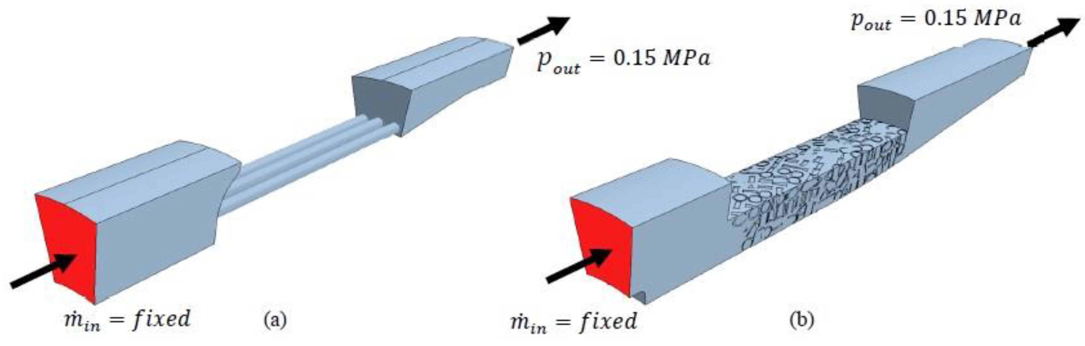
4.4. Simulation Set-Up

As far as the boundary conditions are concerned, a given mass flow rate ${\dot{m}}_{in}$ at 25 °C was imposed at the inlet of the fluid domain for any simulation, while keeping the pressure at the outlet fixed at 0.15 MPa (the variation of the value of $p_{out}$ with the increase of the mass flow rate (see Figure 8) was neglected since the fluid was incompressible). No-slip boundary conditions were imposed on all the fluid–solid interfaces. The fluid properties used in the simulations were computed according to the IAPWS-IF97 standard library, already present in the software options [28].

A second-order scheme with upwind was chosen for the spatial discretization, and a segregated flow model, with an algebraic multigrid (AMG) solver [23], was used to solve the flow equations. Since the problem here is purely hydraulic and the fluid is at a constant temperature, the energy equation was not solved.

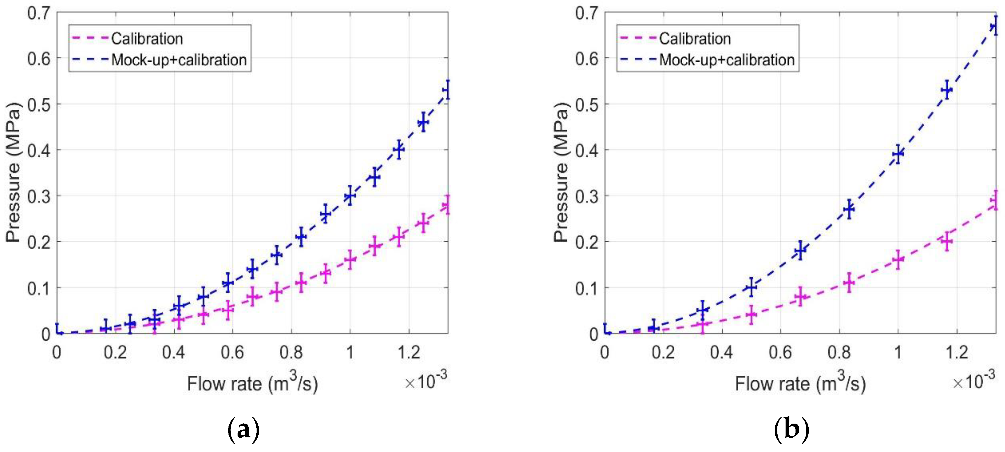
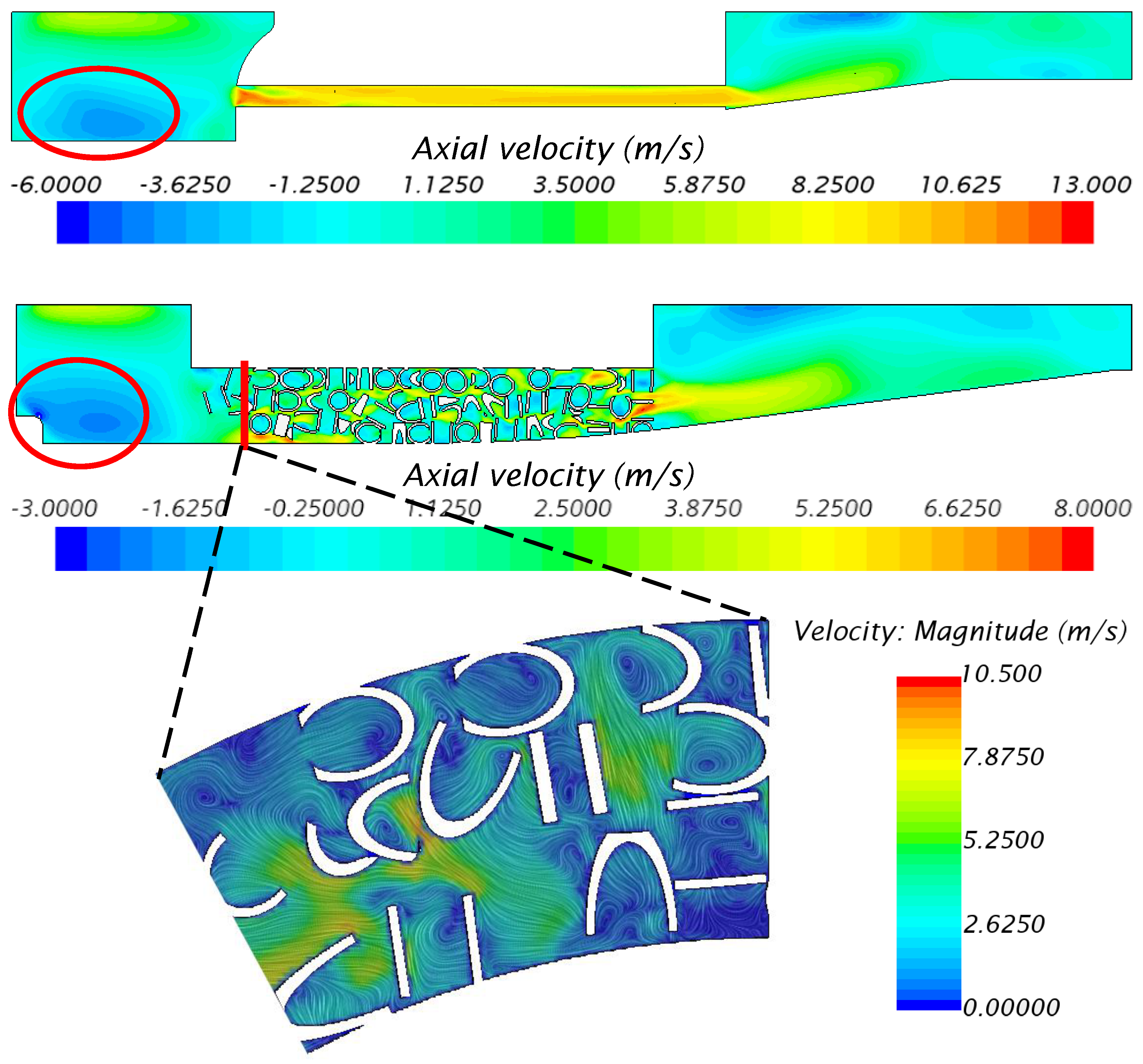
4.5. Model Results and Comparison with Experimental Data

The velocity field, computed on the longitudinal section at 90° from the inlet, is presented in Figure 15 for the MC and RR mock-ups, for an inlet flow rate of 1.16 × 10⁻³ m³/s. As expected, the fluid speed in the MCs was, on average, much higher than that in the RR region, in view of the smaller flow area. The annular inlet manifold kept memory of the fact that there was a single inlet for the fluid; the fluid entered inward and hit the facing wall, redistributing azimuthally around the cavity in both cases (see the details in the circles in Figure 15).

In the MCs, apart from the developing length, the flow was very well aligned with the axial direction (see Figure 15a), as expected. The presence of the high-speed channels drove the jet flow at the outlet of the MC region, which had a strong azimuthal non-uniformity. The high value of the average speed close to the resonator inner surface in the case of the MCs was beneficial for the heat removal, since a non-negligible fraction of the power deposited on the resonator wall affected the region corresponding to the water manifold [8].

The computed flow field in the RR region, reported in Figure 15b, showed a large influence of the local topology of the RR matrix on the velocity distribution, with a significant inhomogeneity both in the azimuthal and in the axial direction. The orientation of the RR had a major effect on the flow; the rings oriented in line with the flow direction could accelerate the local velocity, since the fluid passed through their axial holes, while the rings oriented perpendicularly to the flow direction provided stagnation regions or fluid recirculation. At the RR region outlet, large mixing occurred, as clearly visible in Figure 16a.

The computed pressure maps corresponding to the flow field in Figure 15 are shown in Figure 17, where one can see that, in the MC mock-up (Figure 17a), a large contribution to the pressure losses was due to the inlet of the mini-channel in the annular mixing chamber, i.e., the contribution to the losses of discontinuities of the flow cross-section was significant. On the contrary, in the RR mock-up, the pressure decreased more gradually in the RR porous matrix (see Figure 17b).

Figure 18 reports the comparison between the computed and the measured pressure drop, together with its error band. While the experimental errors were already discussed, the computed error bar which could be estimated from the Richardson extrapolation on different grids was bounded to +0.015 MPa in the worst case (i.e., at 1.16 × 10⁻³ m³/s), as reported in Figure 18b. Apart from the discretization error, another source of uncertainty for the computed results in the case of the RR mock-up came from the effect of the simulated porosity; a first sensitivity analysis on that parameter was performed for a reduced porosity (76.8%), showing a pressure drop difference of +0.01 MPa. In fact, a reduced porosity allowed the formation of “void paths” that became preferential channels with low hydraulic impedance for the fluid.

An excellent agreement between experiment and simulation was found in the cases of both MC (Figure 18a) and RR (Figure 18b) cooling systems, with a relative error which always stayed below 10%. Given that the numerical model had such an excellent prediction of the actual mock-up pressure drop, it constitutes an important validated tool to explore different geometries of the cooling systems, in order to optimize its design. In addition, Figure 18b shows the comparison between the SST k–ω turbulent model, used in our simulations, and the realizable k–ε model suggested by Reference [21]. An excellent agreement between the results of the two models was found; the total pressure drop computed at ~1.16 × 10⁻³ m³/s was within 2% of that computed adopting the SST k–ω model on the same computational grid.

5. Comparative Hydraulic Performance of the Two Cooling Configurations

The MC model was used to simulate the original (already optimized [22]) design with non-circular channel cross-sections shown in Figure 3a and the non-straight axial profile (see Figure 4b), to assess how its pressure drop compares to that of the RR model, as well as to determine, for the two configurations, the maximum flow rate allowing a pressure drop below 0.5 MPa, which is the maximum value allowed for the gyrotron cavity cooling sub-assembly in the actual ITER operating conditions foreseen for the gyrotrons.

The results are shown in Figure 19; the computed pressure drop of the optimized MCs cavity was more than two-fold that of the RR configuration. The reversal of the computed results with respect to the mock-up (pressure drop of the MC mock-up lower than that of the RR mock-up) was due to the different configuration of the MCs. In fact, the flow sections in the case of configuration A (Figure 4a) were much smaller than those in configuration B (Figure 4b) (see also above). Since the number of mini-channels surrounding the cavity was the same, with the same flow rate, the flow rate inside the channels was the same, but the large difference in the section area led to higher fluid velocities in configuration A, with a consequent increase in the distributed pressure drop. Furthermore, the localized pressure drop at the MC inlets increased, in view of the decrease in their section. Moreover, in configuration A, the MCs were slightly longer (~2 mm of difference) since the profile was not straight, while, in configuration B, they had the same length as the WS.

As can be noted from Figure 19, in the case of RRs, pressure drops were always below the defined limit up to 1.5 × 10⁻³ m³/s (above what is considered the maximum operating limit of 1.3 × 10⁻³ m³/s for the gyrotron cavity cooling), while, in the case of MCs, the limit was overcome at 1 × 10⁻³ m³/s (~60 L/min).

6. Conclusions and Perspective

The suitable design, manufacturing, and testing of two different full-size mock-ups (one equipped with MCs, and the other with RRs) of resonance cavities for gyrotrons allowed the measurement of their hydraulic characteristics and, at the same time, the establishment of a solid database for validation of the two corresponding CFD models. After showing an excellent agreement with the measured results, the CFD models were used to directly compare the hydraulic performance of the two cooling configurations when an optimized design was used for the MCs. It turns out that the MC solutions gave a two-fold larger pressure drop when compared to the RR solution, in view of the much higher fluid speed when the cooling channels extended all along the up-taper region.

The main conclusion of the present work is that a maximum flow rate of ~1 × 10⁻³ m³/s (~60 L/min) is allowed in the MC configuration, and a maximum of a flow rate of ~1.5 × 10⁻³ m³/s (~90 L/min) is allowed in the RR configuration, to meet the constraint of a maximum allowable pressure drop of 0.5 MPa along the cavity.

The evaluation of the hydraulic characteristics of the two cooling configurations was one of the two steps needed in order to fairly compare the thermal–hydraulic performance of the two options; the second was the evaluation of their cooling capability. The two planar mock-ups already tested at AREVA [15], without conclusive results, as far as the RR is concerned, were proposed for tests in air in the heating field of the Plataforma Solar de Almeria Solar Furnace SF60. The tests would allow validating the thermal CFD model of the two cooling configurations, in the perspective of a comprehensive comparative thermal–hydraulic performance assessment for the MC and RR cooling solutions.

References

1. ITER Organization. External Heating Systems. Available online: https://www.iter.org/mach/heating (accessed on 18 December 2019).
2. EUROfusion. Fusion on Earth. Available online: https://www.euro-fusion.org/fusion/fusion-on-earth/ (accessed on 18 December 2019).
3. Max Planck Institute for Plasma Physics. Stellarator Theory. Available online: https://www.ipp.mpg.de/ippcms/eng/for/bereiche/stellarator (accessed on 18 December 2019).
4. Kartikeyan, M.V.; Borie, E.; Thumm, M.K.A. Gyrotrons: High Power Microwave and Millimeter Wave Technology, 1st ed.; Springer: Berlin/Heidelberg, Germany, 2004. [Google Scholar]
5. Avramidis, K.A.; Bertinetti, A.; Albajar, F.; Cau, F.; Cismondi, F.; Gantenbein, G.; Illy, S.; Ioannidis, Z.C.; Jelonnek, J.; Legrand, F.; et al. Numerical studies on the influence of cavity thermal expansion on the performance of high-power Gyrotron. IEEE Trans. Electron Devices 2018, 65, 2308–2315. [Google Scholar] [CrossRef]
6. Jelonnek, J.; Aiello, G.; Albaiar, F.; Alberti, S.; Avramidis, K.A.; Bertinetti, A.; Brucker, P.T.; Bruschi, A.; Chclis, I.; Dubray, J.; et al. From W7-X towards ITER and Beyond: 2019 Status on EU Fusion Gyrotron Developments. In Proceedings of the 2019 International Vacuum Electronics Conference (IVEC), Busan, Korea, 29 April–1 May 2019. [Google Scholar]
7. Jelonnek, J.; Aiello, G.; Alberti, S.; Avramidis, K.; Braunmuller, F.; Bruschi, A.; Chelis, J.; Franck, J.; Franke, T.; Gantenbein, G.; et al. Design considerations for future DEMO gyrotrons: A review on related gyrotron activities within EUROfusion. Fusion Eng. Des. 2017, 123, 241–246. [Google Scholar] [CrossRef]
8. Savoldi, L.; Albajar, F.; Alberti, S.; Avramidis, B.A.; Bertinetti, A.; Cau, F.; Cismondi, F.; Gantenbein, G.; Hogge, J.P.; Ioannidis, Z.C.; et al. Assessment and optimization of the cavity thermal performance for the European continuous wave gyrotrons. In Proceedings of the 27th IAEA Fusion Energy Conference (FEC 2018), Gāndhināgar, Indien, 22–27 October 2018. [Google Scholar]
9. Sella, A. Raschig’s Rings. Chem. World 2008, 5, 83. [Google Scholar]
10. Kumar, A.; Kumar, N.; Singh, U.; Khatun, H.; Vyas, V.; Sinha, A.K. Thermal and Structural Analysis and its Effect on Beam-Wave Interaction for 170-GHz, 1-MW Gyrotron Cavity. J. Fusion Energy 2012, 31, 164–169. [Google Scholar] [CrossRef]
11. Karmakar, S.; Sudhakar, R.; Mudiganti, J.C.; Seshadri, R.; Kartikeyan, M.V. Electrical and Thermal Design of a W-Band Gyrotron Interaction Cavity. IEEE Trans. Plasma Sci. 2019, 47, 3155–3159. [Google Scholar] [CrossRef]
12. Savoldi, L.; Bertinetti, A.; Nallo, G.F.; Zappatore, A.; Zanino, R.; Cau, F.; Cismondi, F.; Rozier, Y. CFD analysis of different cooling options for a Gyrotron cavity. IEEE Trans. Plasma Sci. 2016, 44, 3432–3438. [Google Scholar] [CrossRef]
13. Savoldi, L.; Bertinetti, A.; Nallo, G.F.; Zappatore, A.; Zanino, R.; Cau, F.; Cismondi, F.; Rozier, Y. CFD analysis of mini-channels cooling for Gyrotron cavity. In Proceedings of the 26th Symposium on Fusion Engineering (SOFE), Austin, TX, USA, 31 May–4 June 2015. [Google Scholar]
14. Bertinetti, A.; Avramidis, K.; Albajar, F.; Cau, F.; Cismondi, F.; Savoldi, L.; Zanino, R. Multi-physics analysis of a 1 MW gyrotron cavity cooled by mini-channels. Fusion Eng. Des. 2017, 123, 313–316. [Google Scholar] [CrossRef]
15. Bertinetti, A.; Albajar, F.; Cau, F.; Leggieri, A.; Legrand, F.; Perial, E.; Ritz, G.; Savoldi, L.; Zanino, R.; Zappatore, A. Design, test and analysis of a gyrotron cavity mock-up cooled using mini channels. IEEE Trans. Plasma Sci. 2018, 46, 2207–2215. [Google Scholar] [CrossRef]
16. Kalaria, P.; Brücker, P.T.; Ruess, S.; Illy, S.; Avramidis, K.A.; Gantenbein, G.; Thumm, M.; Jelonnek, J. Design Studies of Mini-Channel Cavity Cooling for a 170 GHz, 2 MW Coaxial-Cavity Gyrotron. In Proceedings of the 2019 International Vacuum Electronics Conference (IVEC), Busan, Korea, 29 April–1 May 2019. [Google Scholar]
17. Zhong, W.; Yu, A.; Liu, X.; Tong, Z.; Zhang, H. DEM/CFD-DEM Modelling of Non-spherical Particulate Systems: Theoretical Developments and Applications. Powder Technol. 2016, 302, 108–152. [Google Scholar] [CrossRef]
18. Dong, Y.; Sosna, B.; Korup, O.; Rosowski, F.; Horn, R. Investigation of radial heat transfer in a fixed-bed reactor: CFD simulations and profile measurements. Chem. Eng. J. 2017, 317, 204–214. [Google Scholar] [CrossRef]
19. Wehinger, G.D.; Füterer, C.; Kraume, M. Contact modifications for CFD simulations of fixed-bed reactors: Cylindrical particles. Ind. Eng. Chem. Res. 2017, 56, 87–99. [Google Scholar] [CrossRef]
20. Moghaddam, E.M.; Foumeny, E.A.; Stankiewicz, A.I.; Padding, J.T. Rigid body dynamics algorithm for modeling random packing structures of nonspherical and nonconvex pellets. Ind. Eng. Chem. Res. 2018, 57, 14988–15007. [Google Scholar] [CrossRef] [PubMed] [Green Version]
21. Moghaddam, E.M.; Foumeny, E.A.; Stankiewicz, A.I.; Padding, J.T. Hydrodynamics of narrow-tube fixed bed reactors filled with Raschig Rings. Chem. Eng. Sci. X 2020, 5, 100057. [Google Scholar] [CrossRef]
22. Difonzo, R. Design and Optimization of the Cooling Strategy for a Gyrotron Cavity Equipped with Mini-Channels. Master’s Thesis, Politecnico di Torino, Turin, Italy, 2019. [Google Scholar]
23. Star-CCM+ User’s Guide v 14.02; Siemens PLM Software Inc.: Plano, TX, USA, 2019.
24. Menter, F.R. Two-Equation Eddy-Viscosity Turbulence Models for Engineering Applications. AIAA J. 1994, 32, 1598–1605. [Google Scholar] [CrossRef] [Green Version]
25. Reynolds, O. On the Dynamical Theory of Incompressible Viscous Fluids and the Determination of the Criterion. Philos. Trans. R. Soc. Lond. A 1895, 186, 123–164. [Google Scholar]
26. Versteeg, H.K.; Malalasekera, W. An Introduction to Computational Fluid Dynamics: The Finite Volume Method; Pearson Education Ltd.: Harlow, UK, 2007. [Google Scholar]
27. Ferziger, J.H.; Peric, M. Computational Methods for Fluid Dynamics; Springer: Berlin/Heiderlberg, Germany, 2002. [Google Scholar]
28. The International Association for the Properties of Water and Steam. Available online: http://www.iapws.org/ (accessed on 7 January 2020).
Figure 1. (a) Sketch of the cross-section of a gyrotron, with all the components (modified from https://archive.org/details/gyrotron); (b) computer-aided design (CAD) view of a section of the gyrotron resonance cavity and launcher.
Energies 13 01163 g001
Figure 2. CAD sections of the mock-up equipped with mini-channels (a) and with Raschig rings (b).
Energies 13 01163 g002
Figure 3. Cavity mock-ups equipped with mini-channel (MC): (a) copper cavity with a zoomed-in view showing the mini-channel cross section; (b) nylon cavity.
Energies 13 01163 g003
Figure 4. Sketch of the geometry of the two mock-ups equipped with MCs: configuration A with semicircular + rectangular section (a), and configuration B with circular section (b). For both mock-ups, L = 43 mm and W = 12 mm.
Energies 13 01163 g004
Figure 5. Tomography image of the copper cavity; the red circle evidences the plugged channels.
Energies 13 01163 g005
Figure 6. Cavity equipped with Raschig rings (RRs): (a) view of the ensemble constituted by the cavity, the water-stopper (WS), and the RRs, confined between the two by two containment grids; (b) zoomed-in view of the RR structure generated by discrete element model (DEM) simulation.
Energies 13 01163 g006
Figure 7. (a) Hydraulic test loop with the nylon cavity mock-up equipped with MCs, and, in the red circle, the short hydraulic connector used for the pressure drop calibration; (b) mock-up equipped with RR connected to the loop; (c) sketch of the loop.
Energies 13 01163 g007
Figure 8. Pump inlet and outlet pressure measured in the circuit during the calibration tests and the tests with the mock-ups equipped with the MCs and nylon cavity (a) and RR (b). The error bars on the measured data are reported, together with the respective fits for convenience.
Energies 13 01163 g008
Figure 9. Pressure drop with respect to flow rate evaluated during the calibration tests and the tests with the mock-ups of the cavities equipped with (a) MCs and (b) RRs. The error bars derived from the measured data are reported, together with the corresponding fits of the two datasets.
Energies 13 01163 g009
Figure 10. Schematic of the DEM procedure for the RR matrix generation in a cylindrical sample, as implemented in STAR-CCM+ [23]. a) DEM particles injection phase; b) DEM particles compact matrix; c) definitive matrix after the replacement of the particles with RR.
Energies 13 01163 g010
Figure 11. Reduced domain used for the grid independence study for the (a) MCs and the (b) RRs.
Energies 13 01163 g011
Figure 12. Grid independence analysis on the pressure drop computed for the mock-ups, varying the base size in the water manifolds (a) and the base size in the refined region (b), for a flow rate corresponding to 1.16 × 10⁻³ m3/s in the full mock-up. The red circles highlight the values selected for the simulations in the present analysis.
Energies 13 01163 g012
Figure 13. Section of the computational domain of the mock-up equipped with MCs. Insets: details of the computational mesh.
Energies 13 01163 g013
Figure 14. Computational domain, with boundary conditions, of the mock-up equipped with RRs. Insets: details of the computational mesh.
Energies 13 01163 g014
Figure 15. Axial velocity field computed on a longitudinal section for the mock-up with MCs (a) and RRs (b). Inset: details of the line integral convolution of the component of the velocity tangential to the represented section, colored by the velocity magnitude.
Energies 13 01163 g015
Figure 16. Velocity field map computed on a cross-Section 2 mm apart from the MC (a) and RR (b) regions.
Energies 13 01163 g016
Figure 17. Pressure maps computed on a longitudinal section for the mock-up equipped with MCs (a) and RRs (b).
Energies 13 01163 g017
Figure 18. Comparison of simulation and test results for the mock-up equipped with MCs (a) and RRs (b). The shaded area represents the error band on the experimental results.
Energies 13 01163 g018
Figure 19. Comparison of the pressure drop computed on a cavity equipped with RR and MCs, at different flow rates.
Energies 13 01163 g019