Disturbance Observer-Based Prescribed Performance Fault-Tolerant Control for a Multi-Area Interconnected Power System with a Hybrid Energy Storage System

Abstract

The goal of this study is to develop a disturbance observer-based prescribed performance fault-tolerant controller (PPFTC) for a multi-area interconnected power system (MIPS) with a hybrid energy storage system (HESS). The mathematical model of the MIPS with HESS is introduced first. Then the load disturbance estimation is obtained using a disturbance observer (DO) approach. By introducing two additional functions, the tracking error is bounded to achieve the desired response. The PPFTC is further developed based on the DO ensuring that the area control error (ACE) of the MIPS asymptotically converges to zero. Finally, the effectiveness of the given PPFTC and DO are inspected through the use of the Lyapunov theory and simulated results.

1. Introduction

The requirement for ideal power quality has raised considerable concerns about multi-area power systems, where each interconnected power subsystem shares power with neighboring power subsystems through tie lines [1]. Naturally, the frequency of a power system is the basis of power generation and load balance. The interconnection of power subsystems can improve the frequency stability of the single system, which can also lead to the occurrence of malignant cascading accidents. When the frequency of the system is unstable, the instability travels rapidly through the tie lines, causing large-scale blackouts in serious cases. This can have a serious negative impact on people’s lives and the economy. Therefore, the load frequency control (LFC) of multi-area interconnected power system (MIPS) is particularly important. In recent years, many control strategies have been investigated to solve LFC problems so as to achieve the desired dynamic performance, e.g., proportional-integral- derivative (PID) control [2], optimal control [3], sliding-mode control (SMC) [4], and adaptive control [5].

The primary frequency modulation approach for MIPS maintains the system frequency at the rated value through LFC and makes the area control error (ACE) zero. This is achieved by adjusting the generator sets under the condition of continuously adjustable active power, ensuring that the power generation and load power is matched for the whole system. The grid structure of the power system has increased with the deployment of diverse power system technologies including high-voltage direct current (HVDC) transmission [6], flexible AC transmission technology [7], photovoltaic and wind power generation systems [8], and vehicle-to-grid (V2G) [9]. Nevertheless, the negative effects containing, voltage fluctuation, electric power harmonic pollution, and complex dynamic characteristics [10]. The participation of HESS in frequency modulation can effectively solve the problems of harmonic pollution and voltage instability. For power generation plants, HESS can delay the investment in power generation capacity, improve the performance of frequency modulation and peak regulation, and avoid the risk of extremely low power prices in the market [11]. For power grid companies, energy storage can delay investment in transmission and distribution equipment, alleviate local power grid congestion, provide peak and frequency regulation, voltage support, emergency standby, and black start capability [12]. Electricity sales companies can profit from peak and valley spreads, providing auxiliary services such as peak and frequency modulation. Energy storage can be used with distributed photovoltaic configurations to avoid extreme high price risks in the market, ensure a stable power supply, and avoid power outage risks [13]. Therefore, it is a great necessity to reserve a hybrid energy storage system (HESS) to participate in frequency regulation. Over the past decades, several types of advanced HESS technologies have been developed for the LFC problem [14,15,16,17,18].

At present, the power grid interconnection and increasing dependence on each other make the structure of a power system more complex, and the occurrence of faults inevitable. A breakdown of the power system would have enormous social, economic, and political consequences. The design idea of fault-tolerant control is that when one or a part of the component fails, the system can still run according to the original performance index or the performance index is slightly reduced but within an acceptable range, so as to ensure the normal operation of the system [19,20]. In [21], a fault detection observer associated with the adaptive detection threshold is presented to detect the actuator faults. In [22], an improved sliding mode observer is used to estimate the state of MIPS and sensor faults. Based on the estimated values, a sliding mode fault-tolerant control scheme for sensor faults and external disturbances is designed. To maintain wind turbine generator speed, the author in [23] combines a fault tolerant controller with a proportional-integral (PI) controller to realize an adaptive sliding mode observer to estimate the non-linear faults and eliminate the effects of actuator faults. The above FTC methods usually set a tracking trajectory in advance and then design the controller to achieve the tracking target, or adopt the technique of global SMC to achieve the control of ACE. However, those methods cannot achieve the desired control objectives by selecting some parameters in advance, and their effect mainly depends on the design of the controller and the selection of gain. The prescribed performance control (PPC) can make the convergence speed, overshooting, and steady-state error of the closed-loop system strictly controlled within the required range by introducing the performance function [24]. The PPC scheme is being researched to ensure closed-loop stability by guaranteeing the finite-time convergence of the output error to a desired region [25]. Various control systems have applied PPC, e.g., the singular system [26], the multi-input multi-output (MIMO) nonlinear system [27], the Markovian jump system [28], and chaotic systems [29]. Meanwhile, prescribed performance fault-tolerant control has been widely put into use in practical dynamic systems, such as in inverted pendulum systems [30], satellite systems [31], and power systems [32]. Considering the advantages of the PPC method, it has great potential to be applied to interconnected power systems.

Motivated by the aforementioned research, a disturbance observer based prescribed performance fault-tolerant controller (PPFTC) scheme is designed for the MIPS with HESS. The core idea of the PPC method is to convert the trajectory of the tracking error through the prescribed performance function, so as to ensure that the error can converge to the set range while maintaining the desired transient performance. The responses to two types of power fluctuation are compared to existing methods for LFC of the MIPS to confirm and compare the effectiveness of the PPFTC technique. The main contributions of this work are as follows:

• To the best of the author’s knowledge, so far there have been few reports in published literature that combine prescribed performance control with FTC and apply it to load frequency control of the MIPS;
• Compared to a few existing methods, by designing the finite time disturbance observer, the performance of the observer is improved from asymptotic convergence to finite time convergence.

The paper is presented as follows: The mathematical model of the MIPS, command filter, and the PPC strategy are presented in Section 2. Section 3 details the disturbance observer based prescribed performance fault-tolerant controller. The comparison with several control approaches about MIPS is given in Section 4, followed by conclusions in Section 5. The notations used in this paper are defined in

Table 1. The symbols and acronyms used in the paper.

Parameters	Description
PPFTC	Prescribed performance fault-tolerant control
LFC	Load frequency control
FTC	Fault-tolerant control
SMC	Sliding model control
PID	Proportional-integral- derivative
MIMO	Multi-input multi-output
ACE	Area control error
DO	Disturbance observer
MIPS	Multi-area interconnected power system
V2G	Vehicle-to-grid
HESS	Hybrid energy storage system
HDVC	High-voltage direct current
PPC	Prescribed performance control
CCF	Constrained command filter
$T_{ij}$	Tie-line power synchronization coefficient
$T_{pi}$	Time constant of power system
$T_{gi}$	Time constant of governor
$T_{ti}$	Time constant of turbine
$\Delta P_{tiei}$	Exchange power of tie-lie
$X_{ei}$	Governor valve positon
$P_{di}$	Load disturbance
$P_{gi}$	Generator output power
$P_{ci}$	Power delivered by the HESS to Area i
$K_{pi}$	Power system gain
$\Delta f_i$	Load frequency deviation
${\beta }_i$	Set value of frequency deviation
$AC{E}_i$	Control error of the i-th area.
$R_i$	Speed regulation gain
$K_{AFi}$	Proportional feedback coefficient of frequency deviation

.

2. Problem Formulation and Preliminaries

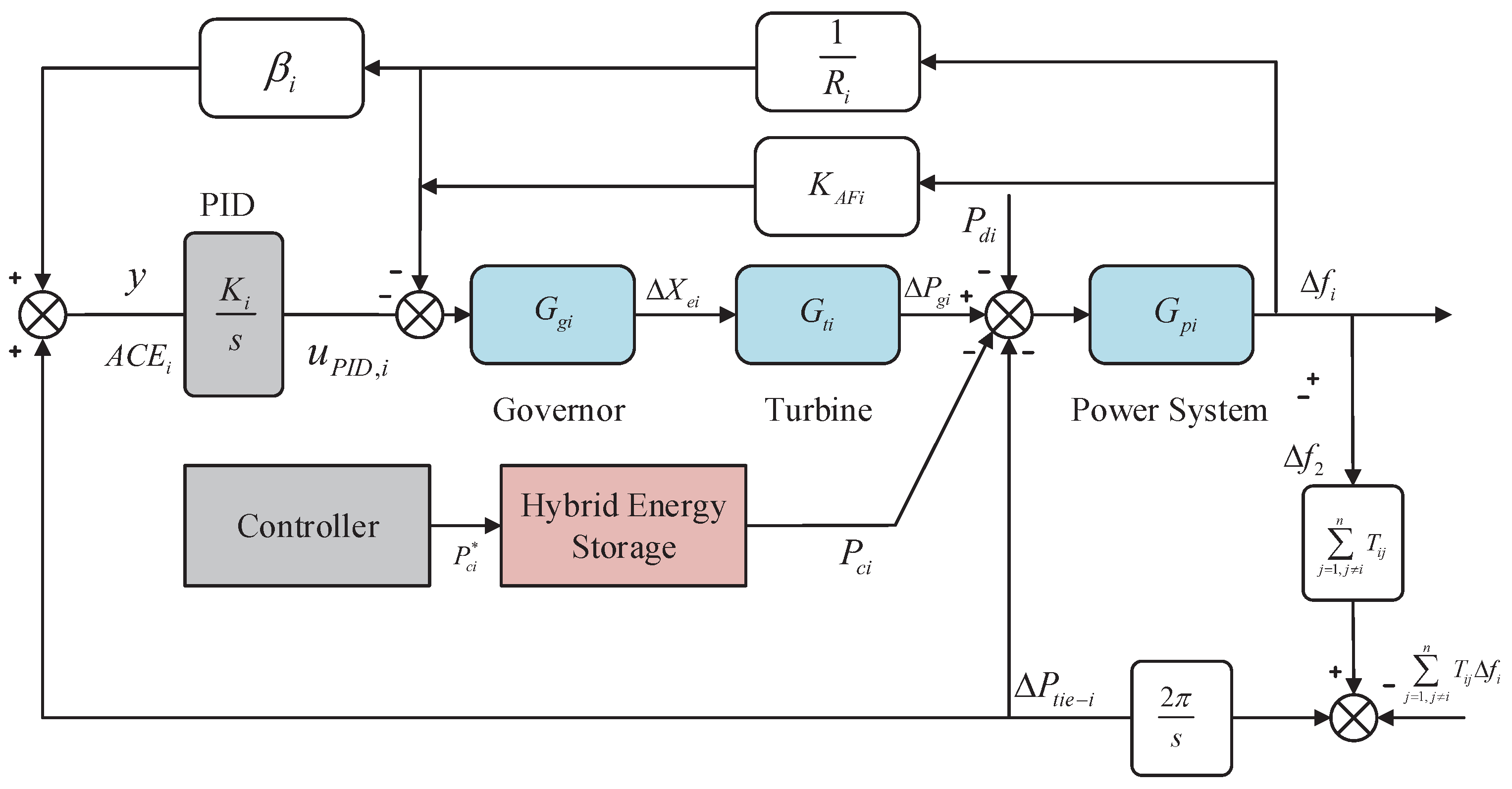
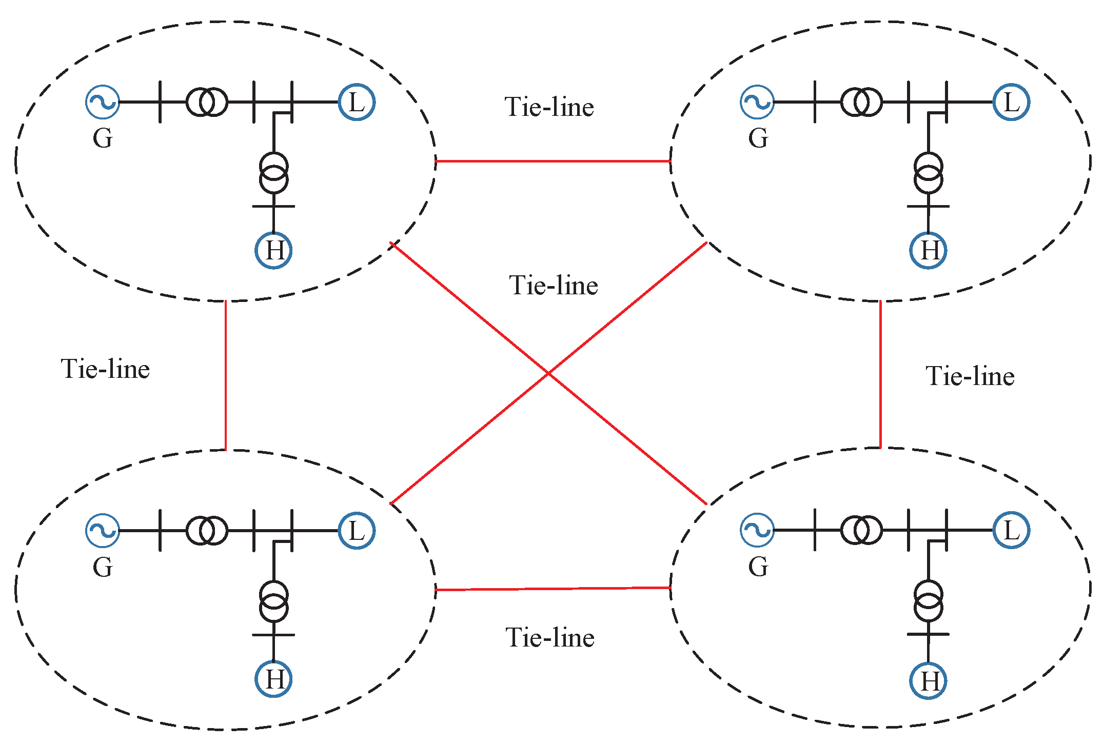
2.1. Modeling of the MIPS

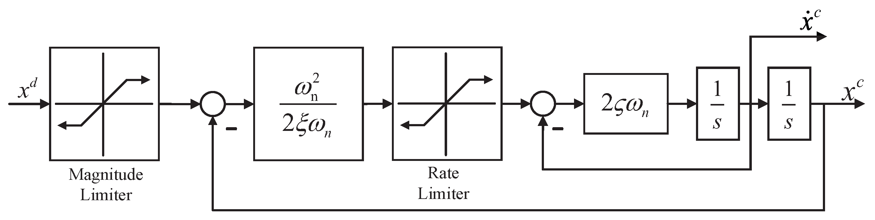
Consider a MIPS consisting of N LFC area, and each area includes the generator, turbine, and governor [10,12]. The i-th control area of the LFC system in the MIPS with HESS is shown in Figure 1. Therefore, each area can be modeled as:

$$\begin{array}{cc}\hfill {\dot{\mathit{x}}}_{\mathit{i}}\left(t\right)& =A_{ii}{\mathit{x}}_{\mathit{i}}\left(t\right)+B_{ii}{u}_i\left(t\right)+B_{ii}{d}_i\left(t\right)+{\mathit{h}}_{\mathit{ij}}\left(t\right),\hfill \end{array}$$

(1)

$$\begin{array}{cc}\hfill y_i\left(t\right)& =C_i{\mathit{x}}_{\mathit{i}}\left(t\right).\hfill \end{array}$$

(2)

where,

$${\mathit{x}}_{\mathit{i}}={\left[\begin{array}{ccccc}\Delta f_i& P_{gi}& X_{ei}& \int AC{E}_i& \Delta P_{tiei}\end{array}\right]}^T,$$

$${\mathbf{h}}_{\mathit{i}\mathit{j}}\left(t\right)=\sum _{j=1,j\ne i}^n\left(A_{ij}{\mathit{x}}_{\mathit{j}}\left(t\right)+B_{ij}{u}_j\left(t\right)\right),$$

$$\begin{array}{c}\hfill A_{ii}=\left[\begin{array}{ccccc}-\frac{1}{T_{pi}}& \frac{K_{pi}}{T_{pi}}& 0& 0& -\frac{K_{pi}}{T_{pi}}\\ 0& -\frac{1}{T_{Ti}}& \frac{1}{T_{Ti}}& 0& 0\\ -\frac{(\frac{1}{R_i}+K_{AFi})}{T_{Gi}}& 0& -\frac{1}{T_{Gi}}& -\frac{1}{T_{Gi}}& 0\\ \frac{{\beta }_i}{R_i}& 0& 0& 0& 1\\ 2\pi {\displaystyle \sum _{j=1,i\ne j}^n}{T}_{ij}& 0& 0& 0& 0\end{array}\right],B_{ii}=\left[\begin{array}{c}\begin{array}{c}-\frac{K_{Pi}}{T_{Pi}}\\ 0\end{array}\\ 0\\ 0\\ 0\end{array}\right],C_i={\left[\begin{array}{c}\frac{{\beta }_i}{R_i}\\ 0\\ 0\\ 0\\ 1\end{array}\right]}^T\end{array},$$

$$\begin{array}{c}\hfill A_{ij}=\left[\begin{array}{ccccc}0& 0& 0& 0& 0\\ 0& 0& 0& 0& 0\\ 0& 0& 0& 0& 0\\ 0& 0& 0& 0& 0\\ -2\pi T_{ij}& 0& 0& 0& 0\end{array}\right].\end{array}$$

(3)

Moreover, $x_i$ is the state vector, $x_j$ is the neighboring state vector of $x_i$, $u_i=P_{ci}$ is the control input which represents the input power of HESS, $y_i=AC{E}_i$ is the output vector, $d_i$ is the load disturbance, $\Delta f_i$, $P_{gi}$, $X_{ei}$, $AC{E}_i$, and $\Delta P_{tiei}$ are the load frequency deviation, the generator output power, the governor valve position, the inner controller output, and the exchange power of tie-lie, respectively, $T_{pi}$, $T_{gi}$, and $T_{ti}$ are the time constants of power system, governor, and turbine, respectively, $R_i$ is the speed regulation gain, ${\beta }_i$ is the set value of frequency deviation, $K_{AFi}$ is the proportional feedback coefficient of frequency deviation, and $T_{ij}$ is the tie-line power synchronization coefficient.

In order to make the power system have a better dynamic performance, we should not only ensure that the frequency deviation of the system tends to zero, but also ensure that the deviation of the tie line switching power is close to zero. The concept of area control error (ACE) in load frequency control is proposed. The ACE of area-i is formulated as:

$$AC{E}_i=\Delta P_{tiei}+{\phi }_i\Delta f_i,$$

(4)

where ${\phi }_i={\beta }_i/R_i$ denotes the frequency deviation constant.

2.2. Command Filter

The controller design adopts a constrained command filter (CCF) to implement the differential calculation of the variables that can solve the problems about input saturation and different expansion. In particular, the work of this paper is based on the assumption that there is no data delay and packet loss. The input is the desired control signal, and the output is the signal and its derivative that the actual control system can achieve. The structure of the CCF is shown in Figure 2 and its state space expression is:

$$\left[\begin{array}{c}{\dot{q}}_1\\ {\dot{q}}_2\end{array}\right]=\left[\begin{array}{c}{q}_2\\ 2\xi {\omega }_n\left[S_R\left(\frac{{\omega }_n^2}{2\xi {\omega }_n}\left(S_M\left(u\right)-q_1\right)\right)-q_2\right]\end{array}\right],$$

(5)

where

$$\left[\begin{array}{c}{q}_1\\ q_2\end{array}\right]=\left[\begin{array}{c}{x}^c\\ {\dot{x}}^c\end{array}\right],u=x^d,$$

and $\xi$ is the damping of the CCF and ${\omega }_n$ is the bandwidth of the CCF. $S_M(·)$ is the amplitude limit and $S_R(·)$ is the rate limit.

Define,

$$z_{i,1}=x_{i,5}-x_{i,5c},$$

(6)

$$z_{i,2}=x_{i,1}-x_{i,1c}.$$

(7)

In addition, $x_{i,5c}=x_{i,5d}$ and $x_{i,5d}$ is the desired frequency deviation. $x_{i,1c}$ is the output of the CCF. Define tracking error ${\mathcal{Z}}_i$ as,

$${\mathcal{Z}}_i=z_{i,1}-{\zeta }_i,$$

(8)

and the ${\zeta }_i$ signal is chosen as

$$\dot{{\zeta }_i}=-k_{i,1}{\zeta }_i+2\pi \sum _{i=1,i\ne j}^n{T}_{ij}{x}_{i,1c}-2\pi \sum _{i=1,i\ne j}^n{T}_{ij}\Delta w_i-x_{i,1d},$$

(9)

where $x_{i,1d}$ is the expected value of $x_{i,1}$.

2.3. Prescribed Performance Control

When designing a controller, it is often expected that the state can converge to its desired trajectory at a fast speed (such as exponential speed). In the process of convergence, the state can not appear to have a high overshoot. In addition, in the steady state process, the state quantity should always remain bounded under the action of interference. The following parts explain the main two process of the prescribed performance control. One is to define a performance function to constrain the tracking error $\mathcal{Z}\left(t\right)$. The other is to make an error transformation to solve the constraint problem.

Through introducing a performance function, the transient and steady state of the tracking error $\mathcal{Z}\left(t\right)$ is set. Define the performance function as follow:

Definition 1.

A smooth function $\rho \left(t\right):{\mathcal{R}}^{+}\to {\mathcal{R}}^{+}$ could be defined as a performance function if:

1) 

$\rho \left(t\right)$ is a positive and decreasing function;

2) 

${lim}_{t\to \infty }\rho \left(t\right)={\rho }_{\infty }>0$.

A widely used performance function that meets definition 1 can be written as:

$$\rho \left(t\right)=({\rho }_0-{\rho }_{\infty })e^{-lt}+{\rho }_{\infty },$$

(10)

where l, ${\rho }_0$, and ${\rho }_{\infty }$ are positive numbers. On the premise that the initial value of $\mathcal{Z}\left(0\right)$ is known, the inequality constraint of the following form is given:

$$\left\{\begin{array}{cc}-M\rho \left(t\right)<\mathcal{Z}\left(t\right)<\rho \left(t\right),\hfill & \mathcal{Z}\left(0\right)>0\hfill \\ -\rho \left(t\right)<\mathcal{Z}\left(t\right)<M\rho \left(t\right),\hfill & \mathcal{Z}\left(0\right)<0\hfill \end{array}\right.,$$

(11)

where $M\in [0,1]$.

When inequality in Equation (11) is satisfied, taking $\mathcal{Z}\left(0\right)>0$ as an example, the error curve will be limited to the area surrounded by $\rho \left(t\right)$ and $-M\rho \left(t\right)$. In addition, according to the decreasing characteristics of the function $\rho \left(t\right)$ and $M\in [0,1]$, the error $\mathcal{Z}\left(t\right)$ will quickly converge to a samll neighborhood of zero under the coaction of both function $\rho \left(t\right)$ and $-M\rho \left(t\right)$. The above process can be explained with reference to Figure 3. ${\rho }_{\infty }$ represents the upper bound of the steady-state error. Therefore, the stable state and transient performance of the output error can be limited by selecting an appropriate performance function $\rho \left(t\right)$.

The constraint inequality shown in Equation (11) is transformed into a non-constrained form by error conversion function, and the conversion function is defined as:

$$S\left(t\right)=\rho \left(t\right)\ell \left(\epsilon \right(t\left)\right).$$

(12)

In Equation (12), $\epsilon \left(t\right)$ is the transformed error. Also, the function $\ell (·)$ should satisfy the following conditions:

(1)

Function $\ell (·)$ is smooth and strictly increasing;

(2)

$$-M<\ell \left(\epsilon \right)<1,\mathcal{Z}\left(0\right)>0;$$

(13)

$$-1<\ell \left(\epsilon \right)<M,\mathcal{Z}\left(0\right)<0;$$

(14)

(3)

$$\left\{\begin{array}{c}\underset{\epsilon \to -\infty }{lim}\ell \left(\epsilon \right)=-M,\hfill \\ \underset{\epsilon \to \infty }{lim}\ell \left(\epsilon \right)=1,\hfill \end{array}\right.\mathcal{Z}\left(0\right)>0;$$

(15)

$$\left\{\begin{array}{c}\underset{\epsilon \to -\infty }{lim}\ell \left(\epsilon \right)=-1,\hfill \\ \underset{\epsilon \to \infty }{lim}\ell \left(\epsilon \right)=M,\hfill \end{array}\right.\mathcal{Z}\left(0\right)<0.$$

(16)

Choose a widely used function $\ell (·)$ which meets all constrains writing as [33]:

$$\ell \left(\epsilon \right)=\left\{\begin{array}{cc}\frac{e^{\epsilon }-M{e}^{-\epsilon }}{e^{\epsilon }+e^{-\epsilon }},\hfill & \mathrm{if}\mathcal{Z}\left(0\right)>0\hfill \\ \frac{M{e}^{\epsilon }-e^{-\epsilon }}{e^{\epsilon }+e^{-\epsilon }},\hfill & \mathrm{if}\mathcal{Z}\left(0\right)<0.\hfill \end{array}\right.$$

(17)

The inverse transformation of the function $\ell (·)$ is:

$$\epsilon \left(t\right)={\ell }^{-1}\left(\frac{\mathcal{Z}\left(t\right)}{\rho \left(t\right)}\right).$$

(18)

Obviously, if $\epsilon \left(t\right)$ is bounded, it can be inferred that the inequality constraint in Equation (11) is established, which can further ensure that the tracking signal meets the requirements of the prescribed performance.

For the development of the PPFTC with the CCF method and disturbance observer, the following assumptions and lemmas are required:

Assumption 1.

$|d_i|\le \overline{d_i}$, $\overline{d_i}$ is a positive number.

Lemma 1.

[34] For any given positive scalars, $0<{\gamma }_0<1$, ${\lambda }_1$, ${\lambda }_2>0$, once the continuous positive definite Lyapunov function $V\left(x\right)$ satisfies the following inequality:

$$\dot{V}\left(x\right)+{\lambda }_{1}V\left(x\right)+{\lambda }_2{V}^{{\gamma }_0}\left(x\right)\le 0,$$

(19)

then the Lyapunov function $V\left(x\right)$ approaches 0 within $T_{reach}$ and the convergence time $T_{reach}$ satisfies that:

$$T_{reach}\le \frac{1}{{\lambda }_1(1-{\gamma }_0)}ln\frac{{\lambda }_1{V}^{1-{\gamma }_0}\left(0\right)+{\lambda }_2}{{\lambda }_2}.$$

(20)

Lemma 2.

[35] For $0<m<1$ and $x_i\in \mathcal{R}$, $i=1,\dots ,l$, the following inequality holds,

$$\sum _{i=1}^l{\left|x_i\right|}^{m+1}\ge {\left(\sum _{i=1}^l{\left|x_i\right|}^2\right)}^{(m+1)/2}.$$

(21)

3. Main Results

3.1. Finite Time Disturbance Observer Design

The observer is designed in this section for the dynamic equation of MIPS with HESS in order to obtain the estimation values about disturbances which can be described by the following form:

$$\widehat{{\mathit{d}}_{\mathit{i}}}=-{\mathcal{K}}_i{\mathit{s}}_{\mathit{i}}-\overline{d_i}sgn\left({\mathit{s}}_{\mathit{i}}\right)-{\parallel A_{ii}{\mathit{x}}_{\mathit{i}}\parallel }_{1}sgn\left({\mathit{s}}_{\mathit{i}}\right)-A_{ii}{\mathit{x}}_{\mathit{i}}-{\eta }_i{sig}^{\lambda }\left({\mathit{s}}_{\mathit{i}}\right),$$

(22)

$${\mathit{s}}_{\mathit{i}}={\mathit{z}}_{\mathit{i}}-{\mathit{x}}_{\mathit{i}},$$

(23)

$${\dot{\mathit{z}}}_{\mathit{i}}=-{\mathcal{K}}_i{\mathit{s}}_{\mathit{i}}-\overline{d_i}sgn\left({\mathit{s}}_{\mathit{i}}\right)-{\parallel A_{ii}{\mathit{x}}_{\mathit{i}}\parallel }_{1}sgn\left({\mathit{s}}_{\mathit{i}}\right)+B_{ii}{u}_i-{\eta }_i{sig}^{\lambda }\left({\mathit{s}}_{\mathit{i}}\right),$$

(24)

where ${\mathcal{K}}_i>0$, ${\epsilon }_i>0$, $0<\lambda <1$, and ${sig}^{\lambda }\left({\mathit{s}}_{\mathit{i}}\right)=\left[\right|{\mathit{s}}_{\mathit{i},\mathbf{1}}{|}^{\lambda }sgn\left({\mathit{s}}_{\mathit{i},\mathbf{1}}\right),|{\mathit{s}}_{\mathit{i},\mathbf{2}}{|}^{\lambda }sgn\left({\mathit{s}}_{\mathit{i},\mathbf{2}}\right),|{\mathit{s}}_{\mathit{i},\mathbf{3}}{|}^{\lambda }sgn\left({\mathit{s}}_{\mathit{i},\mathbf{3}}\right),|{\mathit{s}}_{\mathit{i},\mathbf{4}}{|}^{\lambda }sgn\left({\mathit{s}}_{\mathit{i},\mathbf{4}}\right),|{\mathit{s}}_{\mathit{i},\mathbf{5}}{{|}^{\lambda }sgn\left({\mathit{s}}_{\mathit{i},\mathbf{5}}\right)]}^T$. Therefore, the disturbance tracking error $\tilde{d}$ is defined as:

$$\begin{array}{cc}\hfill \widetilde{{\mathit{d}}_{\mathit{i}}}& =\widehat{{\mathit{d}}_{\mathit{i}}}-{\mathit{d}}_{\mathit{i}}\hfill \\ \hfill & =-{\mathcal{K}}_i{\mathit{s}}_{\mathit{i}}-\overline{d_i}sgn\left({\mathit{s}}_{\mathit{i}}\right)-{∥A_{ii}{\mathit{x}}_{\mathit{i}}∥}_{1}sgn\left({\mathit{s}}_{\mathit{i}}\right)-A_{ii}{\mathit{x}}_{\mathit{i}}-{\eta }_i{sig}^{\lambda }\left({\mathit{s}}_{\mathit{i}}\right)-{\mathit{d}}_{\mathit{i}}\hfill \\ \hfill & =-{\mathcal{K}}_i{\mathit{s}}_{\mathit{i}}-\overline{d_i}sgn\left({\mathit{s}}_{\mathit{i}}\right)-{∥A_{ii}{\mathit{x}}_{\mathit{i}}∥}_{1}sgn\left({\mathit{s}}_{\mathit{i}}\right)-{\eta }_i{sig}^{\lambda }\left({\mathit{s}}_{\mathit{i}}\right)+B_{ii}{u}_i-\dot{{\mathit{x}}_{\mathit{i}}}\hfill \\ \hfill & ={\dot{\mathit{z}}}_{\mathit{i}}-\dot{{\mathit{x}}_{\mathit{i}}}\hfill \\ \hfill & ={\dot{\mathit{s}}}_{\mathit{i}}.\hfill \end{array}$$

(25)

Theorem 1.

Considering the power system in Equation (1) with the external disturbance, a sliding mode-based finite time disturbance observer is designed in Equations (22)–(24). Then the disturbance tracking error $\tilde{d}$ is asymptotically stable. In addition, the convergent process of the disturbance approximation error is guaranteed within a finite time $T_{do1}$.

Proof. 

Considering the following Lyapunov candidate function:

$$V_i=\frac{1}{2}{\mathit{s}}_{\mathit{i}}^T{\mathit{s}}_{\mathit{i}}.$$

(26)

The time derivative of $V_i$ yields:

$$\begin{array}{cc}\hfill {\dot{V}}_i& ={\mathit{s}}_{\mathit{i}}^T{\dot{\mathit{s}}}_{\mathit{i}}\hfill \\ \hfill & ={\mathit{s}}_{\mathit{i}}^T\left(-{\mathcal{K}}_i{\mathit{s}}_{\mathit{i}}-\overline{{\mathit{d}}_{\mathit{i}}}sgn\left({\mathit{s}}_{\mathit{i}}\right)-{\parallel A_{ii}{\mathit{x}}_{\mathit{i}}\parallel }_{1}sgn\left({\mathit{s}}_{\mathit{i}}\right)-A_{ii}{\mathit{x}}_{\mathit{i}}-{\eta }_i{sig}^{\lambda }\left({\mathit{s}}_{\mathit{i}}\right)-{\mathit{d}}_{\mathit{i}}\right)\hfill \\ \hfill & =-{\mathcal{K}}_i{\mathit{s}}_{\mathit{i}}^T{\mathit{s}}_{\mathit{i}}-{\parallel A_{ii}{\mathit{x}}_{\mathit{i}}\parallel }_1{\mathit{s}}_{\mathit{i}}^{T}sgn\left({\mathit{s}}_{\mathit{i}}\right)-{\mathit{s}}_{\mathit{i}}^T{A}_{ii}{\mathit{x}}_{\mathit{i}}-\overline{{\mathit{d}}_{\mathit{i}}}{\mathit{s}}_{\mathit{i}}^{T}sgn\left({\mathit{s}}_{\mathit{i}}\right)-{\mathit{d}}_{\mathit{i}}{\mathit{s}}_{\mathit{i}}^T-{\eta }_i{\mathit{s}}_{\mathit{i}}^T{sig}^{\lambda }\left({\mathit{s}}_{\mathit{i}}\right)\hfill \\ \hfill & \le -{\mathcal{K}}_i{\mathit{s}}_{\mathit{i}}^T{\mathit{s}}_{\mathit{i}}-{\eta }_i{\mathit{s}}_{\mathit{i}}^{T}si{g}^{\lambda }\left({\mathit{s}}_{\mathit{i}}\right)-\overline{d}{\mathit{s}}_{\mathit{i}}^{T}sgn\left({\mathit{s}}_{\mathit{i}}\right)-{\mathit{s}}_{\mathit{i}}^T{\mathit{d}}_{\mathit{i}}\hfill \\ \hfill & \le -\mathcal{K}{\mathit{s}}_{\mathit{i}}^T{\mathit{s}}_{\mathit{i}}-{\eta }_i\sum _{j=1}^5{\left|s_{i,j}\right|}^{\lambda +1}.\hfill \end{array}$$

(27)

According to Lemma 2, it can be further obtained that:

$${\dot{V}}_i\le -{\mathcal{K}}_i{\mathit{s}}_{\mathit{i}}^T{\mathit{s}}_{\mathit{i}}-{\eta }_i{\left(\sum _{j=1}^5{\left|s_{i,j}\right|}^2\right)}^{\frac{\lambda +1}{2}}.$$

(28)

Noting that $V_i=\frac{1}{2}{s}_i^T{s}_i$, the derivation of $V_i$ satisfies that:

$${\dot{V}}_i\le -2{\mathcal{K}}_i{V}_i-2{\eta }_i{V}_i^{\frac{\lambda +1}{2}}.$$

(29)

Therefore, by implementing Lemma 1, the convergence time $T_{doi}$ for the sliding mode variable $s_i$ can be obtained as:

$$T_{doi}\le T_i+\frac{1}{2{\mathcal{K}}_i(1+\frac{\lambda +1}{2})}ln\frac{2{\mathcal{K}}_i{V}^{1-\frac{\lambda +1}{2}}\left(T_i\right)+2{\eta }_i}{2{\eta }_i}.$$

(30)

Consequently, the time derivation of the sliding mode variable $s_i$ converges to 0 within $T_{doi}$ and the disturbance tracking error $\widetilde{{\mathit{d}}_{\mathit{i}}}$ tends to be 0 within $T_{doi}$ as well. □

3.2. Prescribed Performance Fault-Tolerant Controller Design

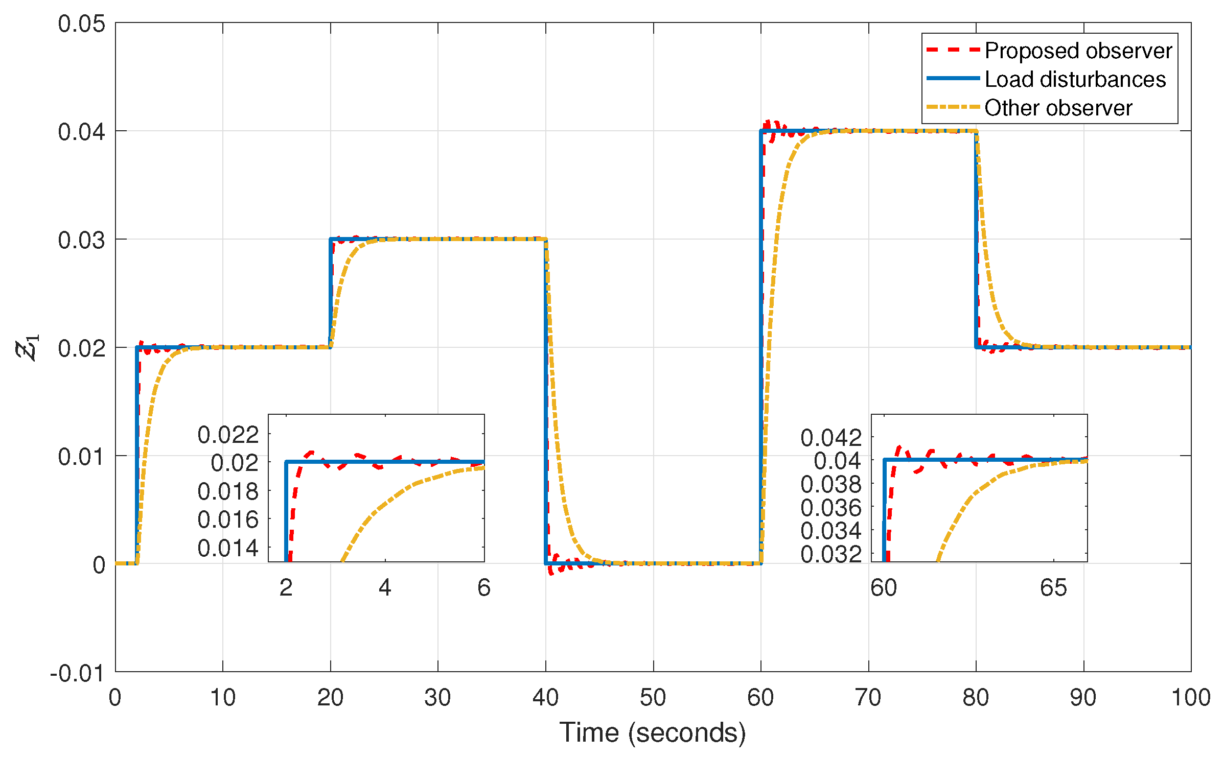
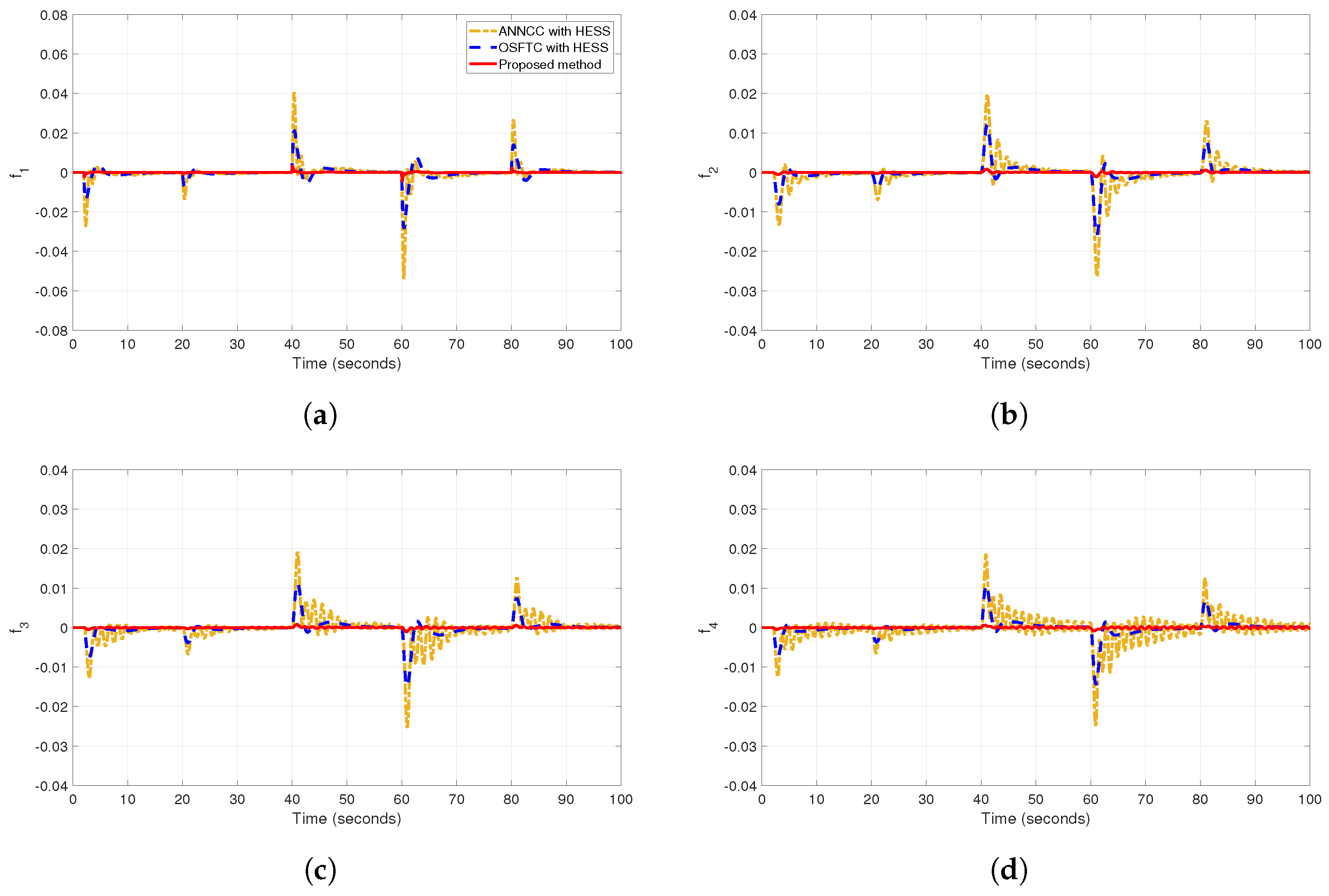
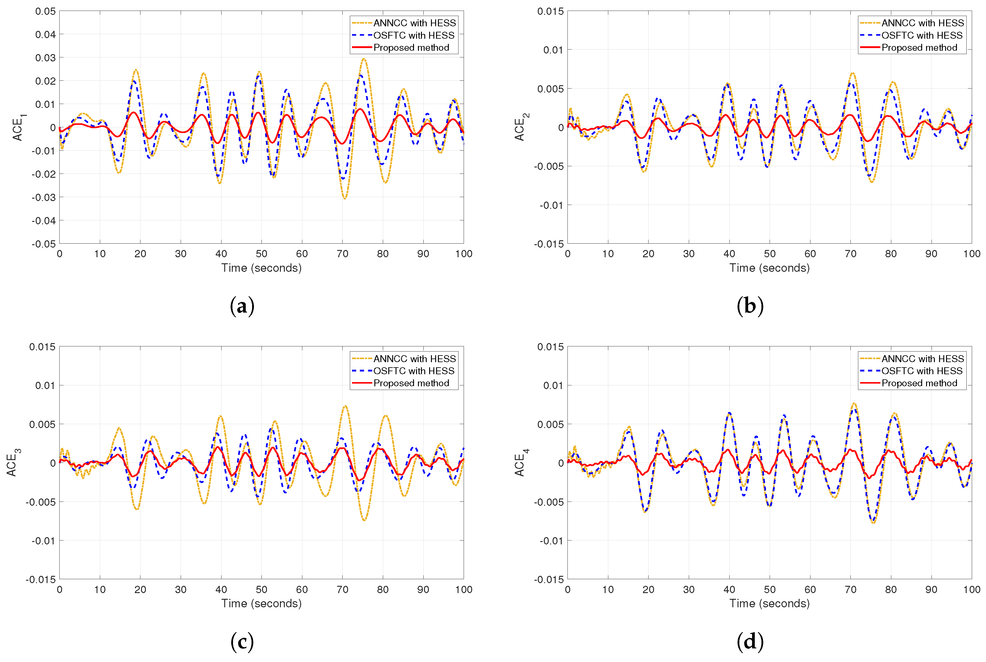
In order to make the power system have a better dynamic performance, not only to ensure the $f_i$ of the MIPS tends to zero, also to ensure that the deviation of the tie line switching power tends to zero. The $AC{E}_i=y_i$ for area i can be expressed as:

$$y_i=\frac{{\beta }_i}{R_i}{x}_{i,1}+x_{i,5},$$

(31)

where,

$${\dot{x}}_{i,1}=-\frac{1}{T_{pi}}{x}_{i,1}+\frac{K_{pi}}{T_{pi}}{x}_{i,2}-\frac{K_{pi}}{T_{pi}}{x}_{i,5}-\frac{K_{pi}}{T_{pi}}{P}_{di}-\frac{K_{pi}}{T_{pi}}{P}_{ci},$$

(32)

$${\dot{x}}_{i,5}=2\pi \left(\sum _{j=1,i\ne j}^n{T}_{ij}{x}_{i,1}-\sum _{j=1,i\ne j}^n{T}_{ij}\Delta w_i\right).$$

(33)

Denoting $f_i\left(x\right)=-\frac{1}{T_{pi}}{x}_{i,1}+\frac{K_{pi}}{T_{pi}}{x}_{i,2}-\frac{K_{pi}}{T_{pi}}{x}_{i,5}$, $F_i=\frac{K_{pi}}{T_{pi}}{P}_{di}$, $b_i=\frac{K_{pi}}{T_{pi}}$. Equation (32) can be simplified as follows:

$${\dot{x}}_{i,1}=f_i\left(x\right)+b_i{u}_i+F_i.$$

(34)

The time derivative of ${\epsilon }_i\left(t\right)$ yields:

$$\begin{array}{c}\dot{{\epsilon }_i}=\frac{\partial {\ell }^{-1}}{\partial ({\mathcal{Z}}_i/\rho )}\frac{1}{\rho }\left({\dot{x}}_{i,5}-{\dot{x}}_{i,5c}-{\dot{\zeta }}_i-\frac{\dot{\rho }{\mathcal{Z}}_i}{\rho }\right)\\ =r_i(2\pi {\displaystyle \sum _{i=1,1\ne j}^n}{T}_{ij}{x}_{i,1}-2\pi {\displaystyle \sum _{j=1,i\ne j}^n}{T}_{ij}\Delta w_i-{\dot{x}}_{i,5c}-{\dot{\zeta }}_i+{\nu }_i),\end{array}$$

(35)

where $r_i=\frac{\partial {\ell }^{-1}}{\partial ({\mathcal{Z}}_i/\rho )}\frac{1}{\rho }$, ${\nu }_i=-\frac{\dot{\rho }{\mathcal{Z}}_i}{\rho }$. Design an integral sliding surface for the inner loop as follows:

$$s_i=z_{i,2}+a_i{\int }_0^t{z_{i,2}}^{m/n}dt,$$

(36)

where n is an odd integer greater than m and both are positive. The form of reaching law is selected as:

$$\dot{s_i}=-k_{i,3}{s}_i-{\tau }_{i}sgn\left(s_i\right),$$

(37)

where $k_{i,3}>0$ and ${\tau }_i>0$ are two positive real numbers. Choose $x_{i,1d}$ as:

$$x_{i,1d}=-k_{i,1}{\zeta }_i+{\dot{x}}_{i,5c}-{\nu }_i-k_{i,2}{\epsilon }_i.$$

(38)

The controller is designed as:

$$u_i=b_i^{-1}\left(-f\left(x\right)+{\dot{x}}_{i,1c}-a_i{z_{i,2}}^{m/n}-k_{i,3}{s}_i-\widehat{d_i}\right).$$

(39)

Theorem 2.

For the power system in Equation (1), if Assumptions 1 and 2 hold, ${\mathcal{Z}}_i$ is going to approach the neighborhood of 0 under the action of prescribed performance. The MIPS can achieve stability under the designed controller in Equations (38) and (39).

Proof. 

Select the Lyapunov function as:

$$V_i=\frac{1}{2r}{\epsilon }_i^2+\frac{1}{2}{s}_i^2.$$

(40)

The time derivative of $V_i$ yields:

$$\begin{array}{ll}{\dot{V}}_i& ={\epsilon }_i·\left(2\pi {\displaystyle \sum _{j=1,i\ne j}^n}{T}_{ij}(x_{i,1}-2\pi \Delta w_i)-{\dot{x}}_{i,5c}-{\dot{\zeta }}_i+{\nu }_i\right)+s_i\left({\dot{z}}_{i,2}+a_i{z_{i,2}}^{m/n}\right)\\ & ={\epsilon }_i·\left(2\pi {\displaystyle \sum _{i=1,i\ne j}^n}{T}_{ij}{z}_{i,2}+k_{i,1}{\zeta }_i-{\dot{x}}_{i,5c}+{\nu }_i+x_{i,1}\right)+s_i\left({\dot{z}}_{i,2}+a_i{z_{i,2}}^{m/n}\right).\end{array}$$

(41)

Substituting Equation (38) into Equation (41), it can be obtained that:

$${\dot{V}}_i=-k_{i,2}·{\epsilon }_i+2\pi \sum _{j=1,1\ne j}^n{T}_{ij}{z}_{i,2}{\epsilon }_i+s_i\left(f\left(x\right)+b_{i}u+d_i-{\dot{x}}_{i,1c}+a_i{z_{i,2}}^{m/n}\right).$$

(42)

Noting that:

$${\epsilon }_i·z_{i,2}\le \frac{1}{2}{\epsilon }_i^2+\frac{1}{2}{z_{i,2}}^2\le \frac{1}{2}{\epsilon }_i^2+\frac{1}{2}{s}_i^2,$$

$$2\pi \sum _{j=1,1\ne j}^n{T}_{ij}·\epsilon ·z_{i,2}\le \pi \sum _{j=1,1\ne j}^n{T}_{ij}\left({\epsilon }^2+z_{i,2}^2\right)\le \pi \sum _{j=1,1\ne j}^n{T}_{ij}\left({\epsilon }_i^2+s_i^2\right).$$

Substituting Equation (39) into Equation (42),

$$\begin{array}{c}{\dot{V}}_1\le -\left(k_{i,2}-\frac{1}{2}\right)·{\epsilon }_i^2+\frac{1}{2}{s}_i^2+s_i\left(f\left(x\right)+b_i{u}_i+d_i-{\dot{x}}_{2,c}+a_i{z}_{i,2}^{m/n}\right)\\ \le -\left(k_{i,2}-\pi {\displaystyle \sum _{i=1,1\ne i}^n}{T}_{ij}\right)·{\epsilon }_i^2-\left(k_{i,3}-\pi {\displaystyle \sum _{i=1,1\ne i}^n}{T}_{ij}\right)s_i^2+s_i\left(d_i-\widehat{d_i}\right).\end{array}$$

It is noted that ${\tilde{d}}_i={\widehat{d}}_i-d_i$ is the disturbance estimation error which could converge to zero asymptotically by choosing a suitable observer. Meanwhile, large enough $k_2,k_3$ can be selected which make the inequality hold,

$$\le -\left(k_{i,2}-\pi \sum _{i=1,1\ne i}^n{T}_{ij}\right)·{\epsilon }_i^2-\left(k_{i,3}-\pi \sum _{i=1,1\ne i}^n{T}_{ij}\right)s_i^2\le 0.$$

(43)

This implies that the transformation error ${\epsilon }_i$ and $z_{i,2}$ are asymptotically stable by using the designed disturbance observer based PPFTC. □

4. Simulations

For simulation studies, a four-area MIPS with HESS is shown in Figure 4, where each area represents the LFC scheme of each power system, and each red line is the tie-line. In order to analyze the stability of the MIPS, system parameters defined in Equation (3) are tabulated in

Table 2. Parameters of a four-area MIPS.

Area i	${\mathit{T}}_{\mathit{g}\mathit{i}}$ (s)	${\mathit{T}}_{\mathit{t}\mathit{i}}$ (s)	${\mathit{R}}_{\mathit{i}}$ (Hz/p.u.Mw)	${\mathit{T}}_{\mathit{i}\mathit{j}}$ (s)	${\mathit{K}}_{\mathit{p}\mathit{i}}$ (Hz/p.u.Mw)	${\mathit{T}}_{\mathit{p}\mathit{i}}$ (s)	${\mathit{\beta }}_{\mathit{i}}$ (Hz/p.u.Mw)	${\mathit{K}}_{\mathit{A}\mathit{F}\mathit{i}}$
1	0.08	0.3	2.4	0.0707	120	20	0.425	1.1
2	0.072	0.33	2.7	0.0707	112.5	25	0.425	1.1
3	0.07	0.35	2.5	0.0707	125	20	0.425	1.1
4	0.085	0.375	2	0.0707	115	15	0.425	1.1

. The parameters of the disturbance observer and prescribed performance FTC is shown in

Table 3. Parameters used in the proposed disturbance observer (DO) and prescribed performance fault-tolerant controller (PPFTC).

Parameters	Values
DO parameters	${\mathcal{K}}_1=50{\mathcal{K}}_2=50{\mathcal{K}}_3=50{\mathcal{K}}_4=50$
	$\overline{d_1}=0.1\overline{d_2}=0.1\overline{d_3}=0.1\overline{d_4}=0.1$
	${\eta }_1=2{\eta }_2=2{\eta }_3=2{\eta }_4=2\lambda =0.5$
PPFTC parameters	$a_1=1a_2=1a_3=1a_4=1$
	$k_{1,1}=12k_{2,1}=12k_{3,1}=12k_{4,1}=12$
	$k_{1,2}=12k_{2,2}=12k_{3,2}=12k_{4,2}=12$
	$k_{1,3}=12k_{2,3}=12k_{3,3}=12k_{4,3}=12$
	${\tau }_1=0.01{\tau }_2=0.01{\tau }_3=0.01{\tau }_4=0.01$
	${\rho }_0=0.02{\rho }_{\infty }=0.01M=0.5m=3n=5$

.

The simulation time is 100 s in total, five successive load disturbances are applied to area 1, with descriptions as follows: +0.02 p.u. (+1500 kW) step disturbance is applied at 2 s; +0.01 p.u. (+750 kW) step disturbance occurs at 20 s; −0.03 p.u. (−2250 kW) step disturbance occurs at 40 s; +0.04 p.u. (+3000 kW) step disturbance occurs at 60 s; −0.02 p.u. (−1500 kW) step disturbance occurs at 80 s. In order to highlight the superiority of the observer designed in this paper, the effect of the observer is tested using the load disturbance as used in [36], and compared with the observer designed in [37]. It can be seen from Figure 5 that the observer designed in this paper converges faster on the estimation of disturbances.

The simulation results of tracking error ${\mathcal{Z}}_1$ is shown in Figure 6. It can be seen from the figure that the magnitude of ${\mathcal{Z}}_1$ is limited by $\rho \left(t\right)$ compared with other method. Meanwhile, the participation of the HESS also reduces the tracking error. Therefore, the dynamic and steady state performance of the ${\mathcal{Z}}_1$ is ensured. Figure 7 and Figure 8 show the changes of ACE under the condition of step disturbances. Figure 9 shows the change of ACE under the condition of renewable power fluctuation in [1]. From the simulations, we can see that in the case of load disturbance, the PPTFC has good control performance, and the out $AC{E}_i$ and $\Delta f_i$ of the MIPS are kept close to zero with a smaller overshoot and faster response compared with the other approaches [10,12].

5. Conclusions

A novel prescribed performance fault-tolerant control scheme with the capability of estimating disturbances was presented to solve the LFC problem of the MIPS with HESS. The disturbance observer developed could estimate the disturbance in a limited time. After using the command filter, the PPFTC was simplified by reducing the calculation of the controller. The dynamic and steady-state performances of the compensated tracking error were verified by the Lyapunov theory. The expected effectiveness of the proposed control scheme was investigated by comparing simulated results with several existing control methods. We note that data delay and packet drop issues, along with sensor/actuator faults are inevitable for MIPS. In future work, our proposed LFC scheme will be improved by addressing the data delay and sensor/actuator faults.

References

1. Zhang, C.; Lin, W.; Ke, D.; Sun, Y. Smoothing tie-line power fluctuations for industrial microgrids by demand side control: An output regulation approach. IEEE Trans. Power Syst. 2019, 34, 3716–3728. [Google Scholar] [CrossRef]
2. Singh, J.; Chattterjee, K.; Vishwakarma, C. Two degree of freedom internal model control-PID design for LFC of power systems via logarithmic approximations. ISA Trans. 2018, 72, 185–196. [Google Scholar] [CrossRef] [PubMed]
3. Alhelou, H.H.; Golshan, M.E.H.; Hatziargyriou, N.D. A decentralized functional observer based optimal LFC considering unknown inputs, uncertainties and cyber-attacks. IEEE Trans. Power Syst. 2019, 34, 4408–4417. [Google Scholar] [CrossRef]
4. Mu, C.; Tang, Y.; He, H. Improved sliding mode design for load frequency control of power system integrated an adaptive learning strategy. IEEE Trans. Ind. Electron. 2017, 64, 6742–6751. [Google Scholar] [CrossRef]
5. Khooban, M.H.; Niknam, T.; Blaabjerg, F.; Davari, P.; Dragicevic, T. A robust adaptive load frequency control for micro-grids. ISA Trans. 2016, 65, 220–229. [Google Scholar] [CrossRef]
6. Pathak, N.; Verma, A.; Bhatti, T.; Nasiruddin, I. Modeling of HVDC tie links and their utilization in AGC/LFC operations of multiarea power systems. IEEE Trans. Ind. Electron. 2018, 66, 2185–2197. [Google Scholar] [CrossRef]
7. Albatsh, F.M.; Mekhilef, S.; Ahmad, S.; Mokhlis, H.; Hassan, M. Enhancing power transfer capability through flexible AC transmission system devices: A review. Front. Inf. Technol. Electron. Eng. 2015, 16, 658–678. [Google Scholar] [CrossRef]
8. Mohanty, A.; Patra, S.; Ray, P.K. Robust fuzzy-sliding mode based UPFC controller for transient stability analysis in autonomous wind-diesel-PV hybrid system. IET Gener. Transm. Distrib. 2016, 10, 1248–1257. [Google Scholar] [CrossRef]
9. Debbarma, S.; Dutta, A. Utilizing electric vehicles for LFC in restructured power systems using fractional order controller. IEEE Trans. Smart Grid 2016, 8, 2554–2564. [Google Scholar] [CrossRef]
10. Xu, D.; Liu, J.; Yan, X.G.; Yan, W. A novel adaptive neural network constrained control for a multi-area interconnected power system with hybrid energy storage. IEEE Trans. Ind. Electron. 2017, 65, 6625–6634. [Google Scholar] [CrossRef]
11. Zhang, S.; Xiong, R.; Sun, F. Model predictive control for power management in a plug-in hybrid electric vehicle with a hybrid energy storage system. Appl. Energy 2017, 185, 1654–1662. [Google Scholar] [CrossRef]
12. Yang, W.; Yu, D.; Xu, D.; Zhang, Y. Observer-based sliding mode FTC for multi-area interconnected power systems against hybrid energy storage faults. Energies 2019, 12, 2819. [Google Scholar] [CrossRef] [Green Version]
13. Fathima, A.H.; Palanisamy, K. Optimization in microgrids with hybrid energy systems—A review. Renew. Sustain. Energy Rev. 2015, 45, 431–446. [Google Scholar] [CrossRef]
14. Attya, A.B.T.; Hartkopf, T. Utilising stored wind energy by hydro-pumped storage to provide frequency support at high levels of wind energy penetration. IET Gener. Transm. Distrib. 2015, 9, 1485–1497. [Google Scholar] [CrossRef] [Green Version]
15. Shankar, R.; Bhushan, R.; Chatterjee, K. Small-signal stability analysis for two-area interconnected power system with load frequency controller in coordination with FACTS and energy storage device. Ain Shams Eng. J. 2016, 7, 603–612. [Google Scholar] [CrossRef] [Green Version]
16. Shankar, R.; Chatterjee, K.; Bhushan, R. Impact of energy storage system on load frequency control for diverse sources of interconnected power system in deregulated power environment. Int. J. Electr. Power Energy Syst. 2016, 79, 11–26. [Google Scholar] [CrossRef]
17. Ranjan, S.; Das, D.C.; Latif, A.; Sinha, N. LFC for autonomous hybrid micro grid system of 3 unequal renewable areas using mine blast algorithm. Int. J. Renew. Energy Res. (IJRER) 2018, 8, 1297–1308. [Google Scholar]
18. Xiong, R.; Cao, J.; Yu, Q. Reinforcement learning-based real-time power management for hybrid energy storage system in the plug-in hybrid electric vehicle. Appl. Energy 2018, 211, 538–548. [Google Scholar] [CrossRef]
19. Shao, X.; Hu, Q.; Shi, Y.; Jiang, B. Fault-tolerant prescribed performance attitude tracking control for spacecraft under input saturation. IEEE Trans. Control. Syst. Technol. 2018, 28, 574–582. [Google Scholar] [CrossRef]
20. Shahbazi, M.; Poure, P.; Saadate, S. Real-time power switch fault diagnosis and fault-tolerant operation in a DFIG-based wind energy system. Renew. Energy 2018, 116, 209–218. [Google Scholar] [CrossRef] [Green Version]
21. Gao, Z.; Zhou, Z.; Jiang, G.; Qian, M.; Lin, J. Active fault tolerant control scheme for satellite attitude systems: Multiple actuator faults case. Int. J. Control. Autom. Syst. 2018, 16, 1794–1804. [Google Scholar] [CrossRef]
22. Su, X.; Liu, X.; Song, Y.D. Fault-tolerant control of multiarea power systems via a sliding-mode observer technique. IEEE/ASME Trans. Mechatron. 2017, 23, 38–47. [Google Scholar] [CrossRef]
23. Lan, J.; Patton, R.J.; Zhu, X. Fault-tolerant wind turbine pitch control using adaptive sliding mode estimation. Renew. Energy 2018, 116, 219–231. [Google Scholar] [CrossRef]
24. Zhang, C.; Ma, G.; Sun, Y.; Li, C. Observer-based prescribed performance attitude control for flexible spacecraft with actuator saturation. ISA Trans. 2019, 89, 84–95. [Google Scholar] [CrossRef] [PubMed]
25. Zhang, J.X.; Yang, G.H. Fuzzy adaptive output feedback control of uncertain nonlinear systems with prescribed performance. IEEE Trans. Cybern. 2017, 48, 1342–1354. [Google Scholar] [CrossRef] [PubMed]
26. Na, J.; Huang, Y.; Wu, X.; Gao, G.; Herrmann, G.; Jiang, J.Z. Active adaptive estimation and control for vehicle suspensions with prescribed performance. IEEE Trans. Control. Syst. Technol. 2017, 26, 2063–2077. [Google Scholar] [CrossRef] [Green Version]
27. Bechlioulis, C.P.; Rovithakis, G.A. Robust adaptive control of feedback linearizable MIMO nonlinear systems with prescribed performance. IEEE Trans. Autom. Control 2008, 53, 2090–2099. [Google Scholar] [CrossRef]
28. Chang, R.; Fang, Y.; Liu, L.; Li, J. Decentralized prescribed performance adaptive tracking control for markovian jump uncertain nonlinear systems with input saturation. Int. J. Adapt. Control. Signal Process. 2017, 31, 255–274. [Google Scholar] [CrossRef]
29. Yang, Q.; Chen, M. Adaptive neural prescribed performance tracking control for near space vehicles with input nonlinearity. Neurocomputing 2016, 174, 780–789. [Google Scholar] [CrossRef]
30. Zhang, J.X.; Yang, G.H. Prescribed performance fault-tolerant control of uncertain nonlinear systems with unknown control directions. IEEE Trans. Autom. Control. 2017, 62, 6529–6535. [Google Scholar] [CrossRef]
31. Hu, Q.; Shao, X.; Guo, L. Adaptive fault-tolerant attitude tracking control of spacecraft with prescribed performance. IEEE/ASME Trans. Mechatron. 2017, 23, 331–341. [Google Scholar] [CrossRef]
32. Kumar, B.K.; Singh, S.; Srivastava, S. A decentralized nonlinear feedback controller with prescribed degree of stability for damping power system oscillations. Electr. Power Syst. Res. 2007, 77, 204–211. [Google Scholar] [CrossRef]
33. Jin, Z.; Zhang, W.; Liu, S.; Gu, M. Command-filtered backstepping integral sliding mode control with prescribed performance for ship roll stabilization. Appl. Sci. 2019, 9, 4288. [Google Scholar] [CrossRef] [Green Version]
34. Bhat, S.P.; Bernstein, D.S. Finite-time stability of continuous autonomous systems. SIAM J. Control Optim. 2000, 38, 751–766. [Google Scholar] [CrossRef]
35. Zhao, L.; Yu, J.; Lin, C.; Ma, Y. Adaptive neural consensus tracking for nonlinear multiagent systems using finite-time command filtered backstepping. IEEE Trans. Syst. Man, Cybern. Syst. 2017, 48, 2003–2012. [Google Scholar] [CrossRef]
36. Dong, L.; Tang, Y.; He, H.; Sun, C. An event-triggered approach for load frequency control with supplementary ADP. IEEE Trans. Power Syst. 2016, 32, 581–589. [Google Scholar] [CrossRef]
37. Guo, C.; Song, C.; Zhao, Y.J.; Wang, J.W. Nonlinear model predictive control for near-Space interceptor based on finite time disturbance observer. Int. J. Aeronaut. Space Sci. 2018, 19, 945–961. [Google Scholar] [CrossRef]
Figure 1. The i-th control area of load frequency control (LFC) in the multi-area interconnected power system (MIPS).
Energies 13 01251 g001
Figure 2. Configuration of the constrained command filter (CCF).
Energies 13 01251 g002
Figure 3. Curve of tracking error and performance function relationship: (a) Z ( 0 ) > 0 and (b) Z ( 0 ) < 0 .
Energies 13 01251 g003
Figure 4. Four area interconnected power system with hybrid energy storage system (HESS).
Energies 13 01251 g004
Figure 5. The value of the disturbance observer.
Energies 13 01251 g005
Figure 6. The time response of the tracking error Z 1 ( t ) (a) response under PID controller with HESS; (b) response under PID controller without HESS; (c) response under proposed controller with HESS; (d) response under proposed controller without HESS.
Energies 13 01251 g006
Figure 7. The A C E i (area control error) of each area subjected to the load disturbances shown in Figure 5: (a) A C E 1 ; (b) A C E 2 ; (c) A C E 3 ; and (d) A C E 4 .
Energies 13 01251 g007
Figure 8. The f i of a four-area MIPS under the load disturbances shown in Figure 5: (a) Δ f 1 ; (b) Δ f 2 ; (c) Δ f 3 ; and (d) Δ f 4 .
Energies 13 01251 g008
Figure 9. The A C E i of each area subjected to the fluctuated renewable power fluction shown in [36]: (a) A C E 1 ; (b) A C E 2 ; (c) A C E 3 ; and (d) A C E 4 .
Energies 13 01251 g009