Modelling the Disaggregated Demand for Electricity in Residential Buildings Using Artificial Neural Networks (Deep Learning Approach) ^†

Abstract

The paper addresses the issue of modelling the demand for electricity in residential buildings with the use of artificial neural networks (ANNs). Real data for six houses in Switzerland fitted with measurement meters was used in the research. Their original frequency of 1 Hz (one-second readings) was re-sampled to a frequency of 1/600 Hz, which corresponds to a period of ten minutes. Out-of-sample forecasts verified the ability of ANNs to disaggregate electricity usage for specific applications (electricity receivers). Four categories of electricity consumption were distinguished: (i) fridge, (ii) washing machine, (iii) personal computer, and (iv) freezer. Both standard ANNs with multilayer perceptron architecture and newer types of networks based on deep learning were used. The simulations included over 10,000 ANNs with different architecture (number of neurons and structure of their connections), type and number of input variables, formulas of activation functions, training algorithms, and other parameters. The research confirmed the possibility of using ANNs to model the disaggregation of electricity consumption based on low frequency data, and suggested ways to build highly optimised models.

1. Introduction

According to the Kyoto protocol of 2008, the electricity used in buildings constitutes 40% of global consumption [1]. A significant part is used in residential buildings. Households in the European Union are estimated to be responsible for more than 27% of the total energy consumption (in 2017), which makes them the second largest source of demand. Only transport exceeds these values and consumes more energy [2].

Knowing the time patterns of energy demand is crucial from the point of view of managing and optimising energy consumption. Optimisation processes are understood as those leading to reduction in electricity consumption and electricity acquisition costs (e.g., in the case of zonal tariffs). It is estimated that potential electricity savings triggered only by consumer behaviour (who possess detailed knowledge about its usage) can range from 5% to 15% [3]. Creating (on this basis) personalised guidelines for the application of electricity receivers can lead to estimated savings of at least 12% [4]. Regardless of the adopted objective, a comprehensive approach requires data for those devices that generate demand. In practice, only aggregate data from smart meters are usually available. They do not provide information on the sources of demand for electricity and, thus, do not provide information on actions that may lead to the optimisation of electricity consumption. The aim of this study is to analyse the possibility of modelling the disaggregated demand for electricity at the level of residential buildings with the use of artificial neural networks (ANNs) based on time patterns, as well as the relation between real and apparent power. The rationale behind the application of different kinds of power consumed by appliances has been confirmed, e.g., by Figueiredo et al. [5] and Esa et al. [6]. The final objective is to predict the activity of a given appliance, understood as its real power consumption above a certain threshold identified in the research. Real power consumption was measured by a sensor located in the plug of a given appliance. Real and apparent powers of total consumption in a house were measured for three single phases separately and were then summed up. As noted by Yu et al. [7], most smart meters in use nowadays make measurements with relatively low frequency, ranging from 1 Hz to 1/900 Hz. It is, therefore, desirable to create systems based on data sampled at a relatively low frequency.

The novelty of the described approach lies in the following:

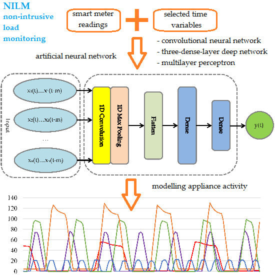
• the application of data with a relatively low sampling rate of 1/600 Hz to model the disaggregated demand for electricity
• the use of different types of ANNs with real and apparent power, as well as selected time and data variables
• the use of the difference between apparent and real power as an input variable in an ANN model.

The estimation of energy consumption for selected key demand sources would potentially enable the implementation of energy management systems without the need to install individual meters for each consumption point. This potentially means not only lower costs for the energy management system but also greater opportunity to increase the popularity (and application) of the systems on the market. Effective (precise) analyses may concern both individual households (end users of energy) [8]–as presented in this study– and the electricity consumption of entire buildings (Liu et al. [9] used the spatiotemporal pattern network (STPN), Henriet et al. [10] showed differences in electricity consumption patterns between residential and commercial buildings pointing out higher periodicity for the latter).

Previous studies on electricity demand in buildings have confirmed its close connection with a number of measurable factors. Chen et al. [1] mention among others: (i) zone temperature measurements, (ii) node temperature measurements, (iii) lighting schedule, (iv) in-room appliances schedule, and (v) room occupancies. Untypical patterns of electricity consumption may be caused by the malfunction of a device (as examined by Rashid et al. [11]). It should be noted that the different structure of energy consumption is related to the legitimacy of using different independent variables. For example, in Canada, 63% of energy is used for space heating, while in the United States this amounts to only 22%. The energy consumption rates for space cooling are 2% and 9% respectively [12]. Therefore, in the first case, weather data are much more desirable in the model than in the second case.

Knowledge of the above-mentioned demand determinants in real time is related to the need for installing technically advanced (expensive) measurement infrastructure connected to the database system. For this reason, numerous studies have focused on the development and implementation of more affordable systems based only on values of total electricity demand. This disaggregation technique is also referred to as non-intrusive load monitoring (NILM), and its origins date back to 1984 [13] and Hart’s publication with the same name [14].

Kotler and Johnson [15] used the factorial hidden Markov model (FHMM) to obtain the percentage of correct answers (called Accuracy—definition in Section 2.5, formula (5)) for the test set (data from a period of two weeks), which ranged from 46.6% to 82% depending on the model and house. High frequency data of up to 15 kHz sub-sampled to a ten-second interval for the purposes of the model evaluation was used in the study. Cominaola et al. [4] extended two-state FHMM with a trace pattern correction by using Iterative Subsequence Dynamic Time Warping (ISDTW). In addition, the research was divided into two periods—summer and winter—due to the seasons’ different energy consumption patterns. The analyses were based on data of a one-minute interval. Bonfigli et al. [16] proposed a modified version of FHMM. Instead of the original algorithm, the additive factorial approximate maximum a posteriori, a new approach based on the structural variational approximation method and the Viterbi algorithm was used for the disaggregation. This translated into an increase in the accuracy of forecasts ranging from 2.5% to 14.9% depending on the case study. Azaza and Wallin [17] used a method based on finite state machines (FSM). The results obtained during the estimation of the activity of seven appliances were characterised by an absolute average error ranging from 5.75% to 21.4% depending on the modelled appliance. To a large extent, this was related to the type of dataset used. The Building-level Fully-labelled Dataset for Electricity Disaggregation (BLUED) yielded results with higher precision than the Reference Energy Disaggregation Dataset (REDD). The authors speculate that this is due to the different intervals between successive samples for the above-mentioned sets of 60 Hz and 1 Hz respectively. Also, the research by Tomkins et al. [18], using the hinge-loss Markov random field (HL-MRF), confirmed the high sensitivity of models to the parameters of acquired data. For REDD and for the Pecan Street dataset (Dataport), the F₁-Measure was 0.722 and 0.505 or 0.503 (depending on the model) respectively. Data from Dataport had a lower sampling rate of 1/60 Hz or 1/3600 Hz. Schirmer et al. [19] tested five different elastic matching algorithms in NILM based on REDD. The minimum variance matching (MVM) achieved the best results measured by both Accuracy and F₁-Measure (definition in Section 2.6, formula (6)) at 87.58% and 89.19% respectively. As noted by Schirmer et al. [19], in contrast to the algorithms they used, approaches based on machine learning require a much larger dataset in order to train the model. De Paiva Penha and Castro [20] applied the convolutional neural network (CNN) approach to model the activity of six appliances in six houses using data from the REDD. The authors used networks with three convolution layers and a single dense layer. Data were divided between the training, validation and test sets in a proportion of 60%, 20%, and 20% respectively. F₁-Measure was 0.93. In one of the proposed models Lie et al. [9] demonstrated the legitimacy of using variables such as indoor and outdoor temperature, which can translate into increased precision for the model. Wu and Wang [21] applied CNN extended by the concatenation operation to separate the feature of the target load by extracting it from the load mixed with the background. The proposed technique was combined with two prevalent networks: Extreme Inception (Xception) and Densely Connected Convolutional Network (DenseNet-121.) The models were positively evaluated in the REDD and UK Domestic Appliance-Level Electricity dataset (UK-DALE) with average F₁-Measure values of 85.1% and 89.0% respectively.

2. Methodology

The study used real data from the Electricity Consumption and Occupancy (ECO) dataset collected from six houses in Switzerland over a period of approximately eight months at a frequency of 1 Hz. The dataset contains, among others, such data provided by smart meters as, the sum of real power over all phases, values of real power, current, and voltage over every phase separately. The plug meters collected the values of real power consumed by an appliance. Detailed information on the structure of energy demand in each property has been given among others in [22]. Since the original frequency was higher than assumed for the purposes of the study, it was necessary to reduce it. The frequently used time interval is 15 min (1/900 Hz⁻¹) [23]. In this study, higher frequency data (with potentially higher practical usefulness) were used. As in [1], the interval of 1/600 Hz⁻¹, i.e., ten minutes, was applied. In order to carry out the transformation described above, arithmetic averages from one-second readings of power consumption for both the overall data and values representing power consumption by specific devices were calculated.

Previous research confirmed the suitability of using different types of power in non-intrusive appliance load monitoring. Dong et al. [24] empirically showed the ranges of real and reactive power values in the case of particular appliances. By applying clustering, they defined the clusters for selected appliances, as well as calculating the average values of both power types. The well-known interdependence between real, reactive and apparent power (its graphic representation is commonly called a power triangle) enables the calculation of each, just by knowing the other two. The data used in this research were based on real and apparent power. The calculation and application of reactive power in the model would mean the use of input variables with strong autocorrelation and high values of variance inflation factor (VIF). It was expected that this would result in the deterioration of the model’s quality. For this reason, only real and apparent power, as well as the differences between them, were used in the research. Figure 1 shows an example of both types of power and their differences for house no. 1.

2.1. Multilayer Perceptron

The creation of ANNs dates back to 1943, when a mathematical model of neurons was developed and presented by McCulloch and Pitts [25] (Figure 2a). In 1958, Rosenblatt [26] published a paper describing the model of a unidirectional network, in which neurons were grouped into successive so-called layers, with signals flowing—as the name indicates—in only one direction (from input to output). A multilayer perceptron (MLP) is composed of three types of layers: (i) a single input layer, (ii) hidden layers, (iii) an output layer (Figure 2b). The last two types of layers are subject to the learning process, which means that the neurons placed in them have the ability to acquire knowledge by modifications in the so-called weights in neurons (real numbers marked as w in Figure 2a).

2.2. Deep Neural Networks

Due to the numerous limitations of the primary architecture, more advanced ANNs based on modified training algorithms, generally referred to as deep neural networks (DNNs), have been gaining popularity in recent years. Under this name, there are many types of networks built on the basis of different types of layers. Although the beginnings of deep learning algorithms in ANNs date back to 1965 [27], they have only recently grown very popular. The reasons behind this surge of interest include technological developments and the increasing use of high-performance graphics processing units (GPUs) to accelerate computing in relation to the CPU. A DNN with a relatively low complexity and high level of similarity to MLP is a network containing dense layers. Its neurons commonly use the rectified linear unit (ReLU) as an activation function (defined by formula (1)). Among other functions, SoftPlus (calculated with formula (2)), SoftSign, SoftMax, Sigmoid, and Tanh are popular. The respective graphs are shown in Figure 3.

f(s) = max(0,s),

(1)

f(s) = ln(1+e^s),

(2)

The multitude of different types of layers in DNN enables the creation of more complex structures. An example is the convolutional neural network (CNN). Commonly used for image classification [28], it also works well in time series analyses [29]. Also noteworthy is their ability to extract features of a low-, mid- and high-level. [30]

Convolutional Neural Network

CNNs are predisposed to extracting high-level features from data by convolution. This is a mathematical operation for merging two datasets. Using the convolution kernel, results are generated in the form of a map of features. In the CNN, in addition to convolution layers, there are typically such layers as: (i) pooling—most often using the maximum or average function (selecting the maximal or calculating the average value from the data area with the dimensions of the filter used)—to reduce the spatial amount of input data [31], (ii) flatten—transforming a two-dimensional dataset into a vector (one-dimensional data) enabling it to be sent to (iii) a dense layer.

DNNs built of three dense layers (3dl-DNN) and CNNs were applied in this research. DNNs use mainly the rectified linear unit (ReLU). The possibility of using other activation functions, such as SoftPlus, SoftSign, SoftMax, Sigmoid, and Tanh, was also tested during the research process. Figure 4 presents the structure of the DNNs used in the research.

The hardware used for the calculations related to the DNNs (both 3dl-DNN and CNN) included a computer equipped with two GPUs with a total computing power of about 26.8 GFLOPS (billions of floating point operations per second), 8704 CUDA cores and thermal design power (TDP) over 500 W. The hardware capacity required by traditional ANNs involved mainly two CPUs with a total of 16 physical cores (32 threads) clocked at 3.6 GHz and TDP rating of 300 W.

2.3. Neural Networks Structure in Modelling Two-State Appliances Activity

Modelling device activity is a classification issue. For this reason, the ANN structure must enable the status of a given device to be assigned to one of the classes (as a minimum). As this research has distinguished between two different states of devices (active and inactive), the final objective reveals a dichotomous problem. There are three popular approaches based on ANN, which involve a different number of neurons in the output layer, and the stage at which the final classification is made. Figure 5 shows their structure, as adapted to the requirements of this study.

Model (a) has two outputs, and only one class must be chosen. This problem can be solved by choosing the class, for which the output value is closer to one. In model (b) only a single neuron is used in an output layer. When its value is equal to zero, it represents one state (e.g., inactivity), whereas when it is equal to one it represents the state of activity. As a continuous activation function used in the neuron, ANN generates output in the form of real numbers in some ranges, e.g., from zero to one for Sigmoid. It is necessary to set a threshold (typically equal to 0.5) below which the answer is understood as zero (inactivity), and over which the answer is considered as one (active). A similar approach is applied in model (c), in which output values of real power consumed by an appliance are assigned to the class by an external classifier working according to the rules applied in model (b), with thresholds as presented in Section 2.5. Model (c) was used in this paper. Figure 6 presents the algorithm for classifying real and estimated appliance activity by the external classifier. In the research, the same threshold was used to assign an appliance activity to one of the two classes on the basis of real data and the modelled device operation. Using two different values of thresholds in the external classifier could generate more accurate results; however, such an approach was rejected for the study due to the risk of not maintaining full objectivity. Two outputs allow the use of such a model in non-dichotomous issues and take into account the situation when two classes can be chosen simultaneously.

2.4. Pre-Assumed Networks Structure and Parameters

The number of neurons in the input layer was adjusted to an optimal set of independent variables (experimentally selected). The output (dense) layer always consisted of one neuron, as all models had a single dependent variable. This study uses three-layer MLPs (single hidden layer) trained by the Broyden–Fletcher–Goldfarb–Shanno (BFGS) algorithm. Sigmoid and Tanh were used as activation functions. The number of neurons in the first two dense layers of the 3dl-DNN was selected experimentally. Dropout units of 0.3 were used after dense layers to reduce interdependent learning among the neurons. In the CNNs, a single convolution layer was applied. The number of epochs for the 3dl-DNN and CNN was limited to 200 and 350 respectively.

2.5. Selection and Preparation of Input and Output Variables of Models

All available data were divided into three sets (training, validation, and test) in the manner introduced by De Paiv Penha and Castro [20], i.e., in a proportion of 60%, 20%, and 20% respectively. Data from the training set were used to train the ANNs. The aim of the validation set was to select the optimal model from all networks of a specific type differing in parameters (e.g., number of neurons, activation functions). The third set—test—was used to determine performance metrics. Due to the methodology used, the tests are an out-of-sample type. The data structure in all three sets was identical.

The independent variables used in this research in the MLP and 3dl-DNN are: (i) the sum of real power over all phases in ten minutes [W], (ii) variable (i) delayed by ten minutes, (iii) the sum of apparent power over all phases in ten minutes [VA], (iv) variable (iii) delayed by ten minutes, (v) the difference between variables (iii) and (i), (vi) variable (v) delayed by ten minutes, (vii) the natural number from the range [1, 144] representing the daily number of ten-minute intervals, (viii) a dummy variable indicating a weekend day (1) and a weekday (0). The structure of datasets (consisting of input variables and an output one) with numerical data is presented in

Table 1. Structure of dataset (sample data for the fridge in house no 1).

Artificial Neural Network (ANN)									External Classifier
Inputs 1								Output	Output
(i)	(ii)	(iii)	(iv)	(v)	(vi)	(vii)	(viii)	Real Power [W]	Active/Inactive 2
96.00	108.00	160.49	166.80	64.49	58.80	24	0	33.35	Active
87.33	79.82	164.70	158.81	77.37	78.99	85	0	1.18	Inactive

¹ The numbers on inputs refer to their numbers and names given in Section 2.5. ² The thresholds were set as presented in Table 2 (10 W in the case of the fridge).

. Due to the artificial neuron texture, as well as the ANN functioning principle, the modelling errors generated by a single cell are multiplied and summed in cells of the next layer. As a result, the total model error is increased. Therefore, the number of input variables was a compromise between a relatively simple structure of the model and the necessity to use the data required for an accurate analysis.

In the case of the CNN, two-dimensional data had to be prepared so that they could be input into the convolution layer. The second dimension consisted of delayed values of the time series. The current (relative to the analysed moment) and five historical values were introduced to obtain two-dimensional data with a total of six elements in the second dimension. Figure 7 shows an example of the transformation of six values of four variables (i) into a 6 × 4 grid. Due to the use of five delayed values of the original time series in the construction of new variables, variables (ii), (iv) and (vi) became redundant. Also, one of the variables (i), (iii) and (v) is redundant. Finally, those CNNs using a new two-dimensional input set based only on variables (i), (v), (vii) and (viii) were used in the research.

The dependent variable was real power measured from a plug (each model made predictions from one plug meter alone). For all properties, the readings from the plug meters did not include the entire period covered by the smart meter measurements. Limiting the analysis to those days for which a full set of data was available (including delayed input variables (ii) and (iv)) would mean that datasets of insufficient size would be used. This would result in both problems with proper ANN training and a decrease in the reliability of the study. For this reason, only selected categories of electricity receivers with a sufficient number of plug meter readings (presented in

Table 2. Four modelled receiver categories.

Receiver Name	Houses	Threshold [W]
Fridge	1, 2, 4, 5, 6	10
Washing machine	1	10
Personal computer	1	14
Freezer	1, 2, 3, 4	10/180 1

¹ The freezer in house no. 4 consumed ca 175 W in idle.

) were analysed. The data were divided into three subsets: training, validation, and test (a similar approach was used by Buddhahai et al. [32]).

Figure 8 shows an example of the arithmetic average of plug meter readings (with a measurement frequency of 1 Hz) recorded in ten minutes. The course of real power consumption is highly cyclical (appliances typically have their own specific work cycles [33]); however, certain differences between cycles might be observed. Some segments in the cycle are constant while others are not. This behaviour of many household appliances is typical and has been described by Seevers et al. [34]. Some detailed differences can easily be observed in the case of electricity receivers. Based on [35], Liu et al. [36] identified four types of devices: (i) on-off appliances (e.g., lamp, toaster), (ii) finite state machines (e.g., washing machine, stove burner), (iii) continuously variable consumer devices (with fluctuations in electricity consumption during activity, e.g., power drill, dimmer lights), and (iv) permanent consumer devices (with constant electricity demand, e.g., hardwired smoke detector, telephone sets). A similar categorisation was introduced by Hamid et al. [37]. In this study, all devices were analysed as two-state appliances (on-off—type (i) or low-high consumption—a subtype of type (ii)). Owing to the fact that over the ten-minute period it is possible that a given device remains both fully active (high demand for electricity) and in a low (or zero) state of current consumption (standby mode or inactive), it was necessary to determine the threshold of real power above which the device was classified as active. Due to the varying electricity demand characteristics of each type of device, these thresholds had to be set individually (third column in Table 2).

On the one hand, the use of a ten-minute period eliminates (to an extent) the problem of real power consumption fluctuations (described by Welikala et al. [38]) through the process of averaging. As a result, it is easier to identify the activity of an appliance. On the other hand, this runs the risk of improperly including several minutes of inactivity into the activity period (and vice versa). Therefore, it was crucial to determine the thresholds as precisely as possible.

2.6. Performance Metrics

The Accuracy and F₁-Measure metrics were used to assess the precision of the model’s operation. In order to determine the second one, two scores called Recall and Precision, defined analogously to those applied by Kolter and Jaakkola [39], were used. Recall presents the percentage share of correctly classified cases. Precision is the percentage of correct classifications only for active appliances. If the designations of the numbers of correct and incorrect estimations according to

Table 3. Designations of the numbers of correct and incorrect estimations.

Appliance Activity
	Estimated	Active	Inactive
Real
Active		TP	FN
Inactive		FP	TN

are adopted, the Recall and Precision scores can be determined using formula (3) and formula (4) [40].

Recall = TP/(TP + FN)

(3)

Precision = TP/(TP + FP)

(4)

Accuracy is the percentage of all correct estimations (without taking into account which device state they concern). It is calculated according to formula (5).

Accuracy = (TP + TN)/(TP + FP + TN + FN)

(5)

F₁-Measure is the geometric mean between Precision and Recall [16]. It is determined using formula (6).

F₁-Measure = 2 × Recall × Precision/(Recall + Precision)

(6)

3. Results

The conducted empirical research showed that (in the DNNs) ReLU is the most effective in most issues analysed. The second-best activation function was SoftPlus. Hyperparameters of the best networks are listed in

Table 4. Hyperparameters of the best deep neural networks (DNNs).

Parameter Name	Description
	Three-Dense-Layer DNN (3dl-DNN)	Convolutional Neural Network (CNN)
Batch size	16 1	16
Loss function	Mean squared error	Mean squared error
Optimiser	Adam	Adam
Beta 1	0.9	0.9
Epsilon (fuzz factor)	1 × 10−8	1 × 10−8
Beta 2	0.999	0.999
Learning rate decay	0	0
Learning rate	0.001	0.001 2

¹ Modelling of fridge activity in house no. 6 was based on a batch size of 32. ² Modelling of fridge activity in house no. 6 was based on learning rate equal to 0.0015.

. The structure parameters are presented in

Table 5. Structure parameters of the best artificial neural networks (ANNs).

Layer/Unit Name	Parameter Name	Value
the best multilayer perceptron (MLP)
Hidden layer (dense)	No. of neurons	11
	Activation function	Tanh
Output layer	No. of neurons	1
	Activation function	Sigmoid
the best three-dense-layer deep neural network (3dl-DNN)
		the freezer in h1 1		the fridge in h6, the freezer in h4			others
1st Dense	No. of neurons	90		70			70
	Activation function	ReLU		SoftPlus			ReLU
1st Dropout unit	Dropout value	0.3		0.3			0.3
2nd Dense	No. of neurons	30		30			30
	Activation function	ReLU		SoftPlus			ReLU
2nd Dropout unit	Dropout value	0.3		0.3			0.3
3rd Dense	No. of neurons	1		1			1
	Activation function	ReLU		SoftPlus			ReLU
the best convolutional neural network (CNN)
		the fridge in h4	the freezer in			the fridge in h6, the freezer in h4		others
			h1		h3
1D Convolution	Activation function	ReLU	ReLU		ReLU	ReLU		ReLU
	Number of filters	8	8		8	10		8
	Filter length	3	3		3	3		3
Max pooling	Pool length	2	2		2	2		2
1st Dense	No. of neurons	80	64		60	64		64
	Activation function	SoftPlus	SoftPlus		SoftPlus	ReLU		ReLU
2nd Dense	No. of neurons	1	1		1	1		1
	Activation function	SoftPlus	SoftPlus		SoftPlus	ReLU		ReLU

¹ h1 is an abbreviation of house no. 1; similarly: h2, h3, h4, h5, and h6.

.

Table 6. Accuracy of disaggregation for three types of artificial neural networks (ANNs): multilayer perceptron (MLP), three-dense-layer deep neural network (3dl-DNN) and convolutional neural network (CNN).

House No. (No. of Test Samples)	ANN Type	Accuracy (No. of Epochs) 1
		Fridge	Washing Machine	Personal Computer	Freezer
1 (1585)	MLP 3dl-DNN CNN	91.17 (151) 93.19 (200) 93.50 (350)	90.41 (88) 71.42 (76) 97.60 (350)	64.67 (146) 64.29 (200) 82.65 (350)	84.92 (377) 66.50 (200) 84.23 (350)
2 (1645)	MLP 3dl-DNN CNN	95.62 (153) 95.99 (200) 95.74 (350)	–	–	92.16 (321) 94.95 (200) 94.04 (350)
3 (1422)	MLP 3dl-DNN CNN	–	–	–	83.26 (224) 76.65 (200) 85.09 (153)
4 (1946)	MLP 3dl-DNN CNN	57.04 (235) 80.47 (200) 58.12 (350)	–	–	77.34 (244) 72.46 (200) 75.23 (350)
5 (2143)	MLP 3dl-DNN CNN	88.80 (140) 89.87 (200) 91.60 (350)	–	–	–
6 (1827)	MLP 3dl-DNN CNN	87.30 (344) 88.29 (200) 89.27 (350)	–	–	–
Weighted average2	MLP 3dl-DNN CNN	83.38 89.23 85.08	90.41 71.42 97.60	64.67 64.29 82.65	84.13 77.54 84.21

¹ Bold font indicates the highest value. ² The quotients of the number of examples in each test set by the number of total cases were used as weights.

presents the results achieved by both the best MLP and 3dl-DNN model based on six input variables: (i), (ii), (v), (vi), (vii), (viii) and the best CNN models using four input variables: (i), (v), (vii), and (viii).

Figure 9 shows two performance metrics (Accuracy and F₁-Measure) calculated separately for each type of appliance (jointly for all the houses in which it was analysed) and for each of the three methods used.

4. Discussion

The analysis of the results achieved by the DNN models shows that the highest precision occurred when estimating the electricity consumption generated by the washing machine. Both the CNN and MLP obtained similar accuracy of estimation. High precision estimation was obtained by all models for fridge electricity consumption. The reasons for this are to be found mainly in the cyclicality of the appliance’s activity, as well as the availability of numerous patterns (at night, devices such as personal computers or washing machines are hardly ever active—similar observations were made by Parson et al. [41]). The worst results were achieved by modelling the energy consumption of the personal computer. It should be assumed that, in addition to the difficulty in creating time patterns of activity using ANNs, this is due to the fact that electricity demand is low in relation to total electricity consumption (Figure 10). Only the CNN was able to obtain acceptable values of accuracy. This could be attributed to the CNN’s ability to recognise complex patterns, as well as its use of input data from a longer time range (five delayed ten-minute intervals). It should be noted, however, that the low value of F₁-Measure was caused by a large number of incorrectly classified cases of personal computer activity, which was recognised as inactive. The opposite estimation error characterised the results obtained by the MLP.

Depending on the modelled appliance activity and the house, different networks achieved the best results. In the case of the CNNs, three were based on the SoftPlus activation function in neurons of dense layers. Other modifications included the number of filters and neurons in the first dense layer. This implies not only the need to train models for each appliance individually, but also to optimise their structure and other parameters.

Three tested models achieved similar accuracy with a slight advantage of the deep learning approach. In 81.8% of simulations, the accuracy of the DNNs was higher than the MLP (in accordance with the numbers in Table 6). The CNN and the 3dl-DDN were the best in 54.5% and 27.3% cases respectively. In 18.2% of the cases, however, the winning model was the MLP.

5. Conclusions and Future Work

Research confirmed the possibility of modelling the disaggregated demand for electricity at the level of individual households (houses) on the basis of low frequency data from smart meters extended by time variables, and real and apparent power.

The simulations showed that when modelling specific appliances, some ANN types may not be able to estimate their activity precisely (e.g., in the case of the fridge in house no. 4). Out of the three models, the one with the highest values of performance metrics can be chosen. It is recommended to create hybrid solutions combining different types of ANNs (and potentially other estimation methods) not only as part of cascading solutions, but primarily as models working in parallel. In this scenario, the winning network would emerge on the basis of tests conducted on the validation dataset.

Future research should be conducted on other ANN models, especially of the DNN type (e.g., with more convolution layers as in [42]—up to two layers—and in [43]—five layers). Due to the high precision of Long Short-Term Memory Networks (LSTMs) in NILM (which has been demonstrated, among others, by Kim and Lee [44] and Le and Kim [45]), models combining both CNNs and LSTMs are also worth exploring (e.g., similar to those proposed by Bhanja and Das [46], Almonacid-Olleros et al. [47], and Kim and Cho [48]). It would be reasonable to create models based on data with a shorter time interval. This would increase the practical value of the models and allow the modelling of the demand for electricity by devices with short time of activity, e.g., microwave ovens. Further research on the possibility of using the presented solution as one component of hybrid models based on the analysis and classification of time patterns of high sampling frequency is also desirable.

The models presented in the study aim primarily at determining the sources (components) of aggregated demand. Their future applications, however, are much wider. For example, their adaptation to the detection of anomalies in the functioning of electricity receivers before their total failure or the subsequent destruction of their technical infrastructure should be considered (similar to those presented in [49]).

References

1. Chen, Y.; Shi, Y.; Zhang, B. Modeling and optimization of complex building energy systems with deep neural networks. Conf. Signals Syst. Comput. 2017, 1368–1373. [Google Scholar]
2. Eurostat. Energy consumption and Use by Households. Available online: https://ec.europa.eu/eurostat/web/products-eurostat-news/-/DDN-20190620-1 (accessed on 10 October 2018).
3. Liu, B.; Luan, W.; Yu, Y. Dynamic time warping based non-intrusive load transient identification. Appl. Energy 2017, 195, 634–645. [Google Scholar]
4. Cominola, A.; Giuliani, M.; Piga, D.; Castelletti, A.; Rizzoli, A. A Hybrid Signature-based Iterative Disaggregation algorithm for Non-Intrusive Load Monitoring. Appl. Energy 2017, 185, 331–344. [Google Scholar] [CrossRef]
5. Figueiredo, M.; De Almeida, A.M.; Ribeiro, B. Home electrical signal disaggregation for non-intrusive load monitoring (NILM) systems. Neurocomputing 2012, 96, 66–73. [Google Scholar] [CrossRef]
6. Xu, F.; Huang, B.; Cun, X.; Wang, F.; Yuan, H.; Lai, L.L.; Vaccaro, A. Classifier economics of Semi-Intrusive Load Monitoring. Int. J. Electr. Power Energy Syst. 2018, 103, 224–232. [Google Scholar] [CrossRef]
7. Yu, J.; Gao, Y.; Wu, Y.; Jiao, D.; Su, C.; Wu, X. Non-Intrusive Load Disaggregation by Linear Classifier Group Considering Multi-Feature Integration. Appl. Sci. 2019, 9, 3558. [Google Scholar] [CrossRef] [Green Version]
8. Biansoongnern, S.; Plungklang, B. Non-Intrusive Appliances Load Monitoring (NILM) for Energy Conservation in Household with Low Sampling Rate. Procedia Comput. Sci. 2016, 86, 172–175. [Google Scholar] [CrossRef] [Green Version]
9. Liu, C.; Akintayo, A.; Jiang, Z.; Henze, G.P.; Sarkar, S. Multivariate exploration of non-intrusive load monitoring via spatiotemporal pattern network. Appl. Energy 2018, 211, 1106–1122. [Google Scholar] [CrossRef]
10. Henriet, S.; Şimşekli, U.; Fuentes, B.; Richard, G. A generative model for non-Intrusive load monitoring in commercial buildings. Energy Build. 2018, 177, 268–278. [Google Scholar] [CrossRef] [Green Version]
11. Rashid, H.; Singh, P.; Stankovic, V.; Stankovic, L. Can non-intrusive load monitoring be used for identifying an appliance’s anomalous behaviour? Appl. Energy 2019, 238, 796–805. [Google Scholar] [CrossRef] [Green Version]
12. Hosseini, S.S.; Agbossou, K.; Kelouwani, S.; Cardenas, A. Non-intrusive load monitoring through home energy management systems: A comprehensive review. Renew. Sustain. Energy Rev. 2017, 79, 1266–1274. [Google Scholar] [CrossRef]
13. Kelly, J.; Knottenbelt, W.; Kelly, J. Metadata for Energy Disaggregation. In Proceedings of the 2014 IEEE 38th International Computer Software and Applications Conference Workshops; Institute of Electrical and Electronics Engineers (IEEE), Västerås, Sweden, 21–25 July 2014; pp. 578–583. [Google Scholar]
14. Hart, G.W. Nonintrusive Appliance Load Data Acquisition Method. In MIT Energy Laboratory Technical Report; MIT: Cambridge, MA, USA, 1984. [Google Scholar]
15. Kolter, J.Z.; Johnson, M.J. REDD: A public data set for energy disaggregation research. In Proceedings of the SustKDD Workshop of Data Mining Applications in Sustainability, San Diego, CA, USA, 21 August 2011. [Google Scholar]
16. Bonfigli, R.; Principi, E.; Fagiani, M.; Severini, M.; Squartini, S.; Piazza, F. Non-intrusive load monitoring by using active and reactive power in additive Factorial Hidden Markov Models. Appl. Energy 2017, 208, 1590–1607. [Google Scholar] [CrossRef]
17. Azaza, M.; Wallin, F. Finite State Machine Household’s Appliances Models for Non-intrusive Energy Estimation. Energy Procedia 2017, 105, 2157–2162. [Google Scholar] [CrossRef]
18. Tomkins, S.; Pujara, J.; Getoor, L. Disambiguating Energy Disaggregation: A Collective Probabilistic Approach. In Proceedings of the Twenty-Sixth International Joint Conference on Artificial Intelligence, Melbourne, Australia, 19–25 August 2017; pp. 2857–2863. [Google Scholar]
19. Schirmer, P.A.; Mporas, I.; Paraskevas, M. Energy Disaggregation Using Elastic Matching Algorithms. Entropy 2020, 22, 71. [Google Scholar] [CrossRef] [Green Version]
20. Penha, D.D.P.; Castro, A.R.G. Home Appliance Identification for Nilm Systems Based on Deep Neural Networks. Int. J. Artif. Intell. Appl. 2018, 9, 69–80. [Google Scholar] [CrossRef]
21. Wu, Q.; Wang, F. Concatenate Convolutional Neural Networks for Non-Intrusive Load Monitoring across Complex Background. Energies 2019, 12, 1572. [Google Scholar] [CrossRef] [Green Version]
22. Beckel, C.; Kleiminger, W.; Cicchetti, R.; Staake, T.; Santini, S. The ECO data set and the performance of non-intrusive load monitoring algorithms. In Proceedings of the 1st ACM Conference on Embedded Systems for Energy-Efficient Buildings—BuildSys, Memphis, TN, USA, 5–6 November 2014; pp. 80–89. [Google Scholar]
23. Liu, C.; Jiang, Z.; Akintayo, A.; Henze, G.P.; Sarkar, S. Building Energy Disaggregation using Spatiotemporal Pattern Network. In Proceedings of the 2018 Annual American Control Conference (ACC), Milwaukee, WI, USA, 27–29 June 2018; pp. 1052–1057. [Google Scholar]
24. Dong, M.; Meira, P.C.; Xu, W.; Chung, C.Y. Non-Intrusive Signature Extraction for Major Residential Loads. IEEE Trans. Smart Grid 2013, 4, 1421–1430. [Google Scholar] [CrossRef]
25. McCulloch, W.S.; Pitts, W. A logical calculus of the ideas immanent in nervous activity. Bull. Math. Boil. 1943, 5, 115–133. [Google Scholar] [CrossRef]
26. Rosenblatt, F. The perceptron: A probabilistic model for information storage and organization in the brain. Psychol. Rev. 1958, 65, 386–408. [Google Scholar] [CrossRef] [Green Version]
27. Ivakhnenko, A.G.; Lapa, V.G. Cybernetic Predicting Devices; CCM Information Corp.: New York, NY, USA, 1965. [Google Scholar]
28. Zhang, C.-L.; Wu, J. Improving CNN linear layers with power mean non-linearity. Pattern Recognit. 2019, 89, 12–21. [Google Scholar] [CrossRef]
29. Debayle, J.; Hatami, N.; Gavet, Y. Classification of time-series images using deep convolutional neural networks. In Proceedings of the Tenth International Conference on Machine Vision (ICMV 2017), Vienna, Austria, 13–15 November 2017; p. 106960. [Google Scholar]
30. Wang, K.; Li, K.; Zhou, L.-Q.; Hu, Y.; Cheng, Z.; Liu, J.; Chen, C. Multiple convolutional neural networks for multivariate time series prediction. Neurocomputing 2019, 360, 107–119. [Google Scholar] [CrossRef]
31. Patterson, J.; Gibson, A. Deep Learning: A Practitioner’s Approach, 1st ed.; O’Reilly Media, Inc.: Sebastopol, CA, USA, 2017; pp. 125–140. [Google Scholar]
32. Buddhahai, B.; Wongseree, W.; Rakkwamsuk, P. A non-intrusive load monitoring system using multi-label classification approach. Sustain. Cities Soc. 2018, 39, 621–630. [Google Scholar] [CrossRef]
33. Cui, G.; Liu, B.; Luan, W. Neural Network with Extended Input for Estimating Electricity Consumption Using Background-based Data Generation. Energy Procedia 2019, 158, 2683–2688. [Google Scholar] [CrossRef]
34. Seevers, J.-P.; Johst, J.; Weiß, T.; Meschede, H.; Hesselbach, J. Automatic Time Series Segmentation as the Basis for Unsupervised, Non-Intrusive Load Monitoring of Machine Tools. Procedia CIRP 2019, 81, 695–700. [Google Scholar] [CrossRef]
35. Zoha, A.; Gluhak, A.; Imran, M.A.; Rajasegarar, S. Non-Intrusive Load Monitoring Approaches for Disaggregated Energy Sensing: A Survey. Sensors 2012, 12, 16838–16866. [Google Scholar] [CrossRef] [PubMed] [Green Version]
36. Liu, Y.; Wang, X.; Zhao, L.; Liu, Y. Admittance-based load signature construction for non-intrusive appliance load monitoring. Energy Build. 2018, 171, 209–219. [Google Scholar] [CrossRef]
37. Hamid, O.; Barbarosou, M.; Papageorgas, P.; Prekas, K.; Salame, C.-T. Automatic recognition of electric loads analyzing the characteristic parameters of the consumed electric power through a Non-Intrusive Monitoring methodology. Energy Procedia 2017, 119, 742–751. [Google Scholar] [CrossRef]
38. Welikala, S.; Thelasingha, N.; Akram, M.; Ekanayake, M.P.B.; Godaliyadda, G.M.R.I.; Ekanayake, J.B. Implementation of a robust real-time non-intrusive load monitoring solution. Appl. Energy 2019, 238, 1519–1529. [Google Scholar] [CrossRef]
39. Kolter, J.; Jaakkola, T. Approximate inference in additive factorial HMMs with application to energy disaggregation. J. Mach. Learn. Res. 2012, 22, 1472–1482. [Google Scholar]
40. Xia, M.; Liu, W.; Wang, K.; Zhang, X.; Xu, Y. Non-intrusive load disaggregation based on deep dilated residual network. Electr. Power Syst. Res. 2019, 170, 277–285. [Google Scholar] [CrossRef]
41. Parson, O.; Ghosh, S.; Weal, M.; Rogers, A. An unsupervised training method for non-intrusive appliance load monitoring. Artif. Intell. 2014, 217, 1–19. [Google Scholar] [CrossRef]
42. Kelly, J.; Knottenbelt, W. Neural NILM. In Proceedings of the 2nd ACM International Conference on Embedded Systems for Energy-Efficient Built Environments, Seoul, South Korea, 4–5 November 2015; pp. 55–64. [Google Scholar]
43. Zhang, C.; Zhong, M.; Wang, Z.; Goddard, N.; Sutton, C. Sequence-to-point learning with neural networks for non-intrusive load monitoring. arXiv 2017, arXiv:1612.09106. [Google Scholar]
44. Kim, J.-G.; Lee, B. Appliance Classification by Power Signal Analysis Based on Multi-Feature Combination Multi-Layer LSTM. Energies 2019, 12, 2804. [Google Scholar] [CrossRef] [Green Version]
45. Le, T.-T.-H.; Kim, H. Non-Intrusive Load Monitoring Based on Novel Transient Signal in Household Appliances with Low Sampling Rate. Energies 2018, 11, 3409. [Google Scholar] [CrossRef] [Green Version]
46. Deep Learning-based Integrated Stacked Model for the Stock Market Prediction. Int. J. Eng. Adv. Technol. 2019, 9, 5167–5174. [CrossRef]
47. Almonacid-Olleros, G.; Almonacid, G.; Fernández-Carrasco, J.I.; Quero, J.M. Opera.DL: Deep Learning Modelling for Photovoltaic System Monitoring. Proceedings 2019, 31, 50. [Google Scholar] [CrossRef] [Green Version]
48. Kim, T.-Y.; Cho, S.-B. Predicting residential energy consumption using CNN-LSTM neural networks. Energy 2019, 182, 72–81. [Google Scholar] [CrossRef]
49. Dinesh, C.; Welikala, S.; Liyanage, Y.; Ekanayake, M.P.B.; Godaliyadda, R.I.; Ekanayake, J. Non-intrusive load monitoring under residential solar power influx. Appl. Energy 2017, 205, 1068–1080. [Google Scholar] [CrossRef]
Figure 1. Graph of real and apparent power and their differences for house no. 1.
Energies 13 01263 g001
Figure 2. Model of: (a) neuron; (b) multilayer perceptron.
Energies 13 01263 g002
Figure 3. Graphs of six tested activation functions.
Energies 13 01263 g003
Figure 4. The structure of the deep neural networks (DNNs) used in the research.
Energies 13 01263 g004
Figure 5. The structure of artificial neural network (ANN)-based models used in dichotomous classification problems.
Energies 13 01263 g005
Figure 6. Algorithm for classifying real and estimated activity by external classifier on the basis of threshold.
Energies 13 01263 g006
Figure 7. An example of the transformation of four time series into a two-dimensional variable.
Energies 13 01263 g007
Figure 8. Electricity consumption generated by fridges.
Energies 13 01263 g008
Figure 9. Models’ performance in terms of: (a) accuracy (%), (b) F1-measure (%).
Energies 13 01263 g009
Figure 10. Total electricity consumption generated by a PC over four days.
Energies 13 01263 g010