Regression Models for the Evaluation of the Techno-Economic Potential of Organic Rankine Cycle-Based Waste Heat Recovery Systems on Board Ships Using Low Sulfur Fuels ^†

Abstract

When considering waste heat recovery systems for marine applications, which are estimated to be suitable to reduce the carbon dioxide emissions up to 20%, the use of organic Rankine cycle power systems has been proven to lead to higher savings compared to the traditional steam Rankine cycle. However, current methods to estimate the techno-economic feasibility of such a system are complex, computationally expensive and require significant specialized knowledge. This is the first article that presents a simplified method to carry out feasibility analyses for the implementation of organic Rankine cycle waste heat recovery units on board vessels using low-sulfur fuels. The method consists of a set of regression curves derived from a synthetic dataset obtained by evaluating the performance of organic Rankine cycle systems over a wide range of design and operating conditions. The accuracy of the proposed method is validated by comparing its estimations with the ones attained using thermodynamic models. The results of the validation procedure indicate that the proposed approach is capable of predicting the organic Rankine cycle annual energy production and levelized cost of electricity with an average accuracy within 4.5% and 2.5%, respectively. In addition, the results suggest that units optimized to minimize the levelized cost of electricity are designed for lower engine loads, compared to units optimized to maximize the overall energy production. The reliability and low computational time that characterize the proposed method, make it suitable to be used in the context of complex optimizations of the whole ship’s machinery system.

1. Introduction

The increasing awareness of the environmental impact of the shipping industry is pushing the development of novel solutions to reduce the emission of pollutants from ships. In this context, the International Maritime Organization (IMO) recently introduced a novel legislation framework constraining the emissions of nitrogen oxides (NO_x) [1] and sulfur oxides (SO_x) [2], and set the vision to reduce the greenhouse gas (GHG) emissions by 50% compared to the emissions levels of 2008 by 2050 [3].

Several alternative solutions can, in theory, lead to a reduction of the emissions from shipping, one of them being the use of liquefied natural gas (LNG) [4]. Compared to the use of traditional heavy fuel oils (HFO), the use of LNG leads to substantial reductions in the NO_x and SO_x emissions [5]: the former can be reduced up to 85% thanks to the lean combustion process, while the latter are almost completely eliminated, because LNG does not contain sulfur. Additionally, a significant potential to reduce the environmental impact of ships lies in the possibility to recover the waste heat released by the ship’s engine system. According to the work from Bouman et al. [6], the implementation of waste heat recovery (WHR) solutions on board a vessel can result in a reduction of the carbon dioxide (CO₂) emissions by up to 20%.

Waste-to-heat recovery solutions are particularly attractive for cruise ships [7,8], because such ships require a significant amount of heat for internal uses, while waste-to-power solutions are the most commonly investigated for containerships and tankers, among others [9].

The organic Rankine cycle (ORC) power system has been identified as a promising solution for waste-to-power recovery applications on board vessels [9], because it enables the attainment of higher design power outputs [10] and improved off-design efficiencies [11], in comparison with the traditional steam Rankine cycle technology.

Most of the previous works dealing with the optimal design of ORC power cycles for maritime applications have been following a model-driven approach, meaning that they rely on the use of numerical models based on the laws of thermodynamics, and validated by comparison with experimental data, when available. Such models are then used to investigate the performance of the unit under different design and off-design conditions.

The development of suitable numerical models to predict the performance and optimal design of ORC units for maritime applications is, however, a challenging task, because the designer needs to account for a multitude of aspects, including the availability of multiple waste heat sources, the ORC off-design performance, the ship sailing profile, the impact of the WHR unit on the engine’s performance, and the presence of dynamic instabilities, among others.

In this regard, Soffiato et al. [12] described a procedure to integrate the use of multiple waste heat sources on board a LNG-carrier. Baldi et al. [13] discussed multiple optimization approaches and concluded that the ship sailing profile needs to be accounted for during the ORC design procedure in order to maximize the annual energy production. Michos et al. [14] highlighted the impact of the additional backpressure supplied to the exhaust line of a marine engine by the implementation of a WHR unit, while Baldasso et al. [15] suggested that constraining the maximum backpressure on the exhaust side of the ORC WHR boiler leads to a significant reduction of the attainable power output from the recovery unit. Lastly, Rech et al. [16] pointed out the importance of carrying out dynamic simulations to ensure that the system is correctly sized and is capable of reaching steady-state operation under a wide range of engine operating conditions.

The downsides of the approach followed by the aforementioned works lie in the model complexity, and in the computational time required to carry out the simulations, which increases as more aspects are taken into account. These approaches are therefore commonly used in a limited number of case studies, but are not suitable to carry out preliminary estimations of the potential for installing ORC-based WHR units on board a wide range of vessels.

To cover this need, another range of studies are available in the literature. Other authors, in fact, aimed at deriving simplified methodologies to estimate the performance of ORC units. Among these works, Liu et al. [17] proposed an equation to estimate the thermal efficiency of an ORC unit based on the working fluid evaporation, condensation, and critical temperatures. Kuo et al. [18] correlated the Jakob number with the attainable ORC thermal efficiency, while Wang et al. [19] used the Jakob number in predictive models to estimate the ORC thermal and exergy efficiencies. Larsen et al. [20] proposed the use of multiple regression models to predict the ORC thermal efficiency given the boundary conditions of the process. Lecompte et al. [21] focused on the cycle second law efficiency and derived a simplified correlation to estimate its maximum value for a given waste heat source. Lastly, Palagi et al. [22] developed surrogate models based on a neural network approach to carry out multi-objective optimization of a small-scale ORC unit, showing that the computational time could be reduced by two orders of magnitude in comparison with the traditional optimization approach.

These works pose a solid foundation for the rapid estimation of the prospects for installing an ORC unit, but have two limitations: (1) they aim at estimating the unit efficiency, rather than its power output, which is the key performance indicator in case of WHR applications, and (2) they are suitable for design conditions estimations only, thus, they do not consider the off-design performance of the unit, which is of key importance when considering the maritime application, because the waste heat availability changes according to the engine load.

To the best of the authors’ knowledge, only one previously published work describes a simplified method to estimate the off-design performance of an ORC unit: Dickes et al. [23] carried out experimental and numerical investigations on a 2 kW_el ORC system featuring a scroll expander and proposed a set of equations to characterize the optimal off-design operation of the ORC system. As the equations were derived based on a specific unit, their general applicability is, however, not guaranteed. In addition, the off-design characterization of ORC units featuring volumetric expanders is not comparable to the one of units featuring turbo-expanders (i.e., units tailored for maritime applications).

This work aims at deriving a set of models for the quick and accurate prediction of the annual energy production and economic attractiveness of ORC units optimized for marine applications, considering low-sulfur fuels. The models were derived by numerical regression of a synthetic database of optimized ORC units and their effectiveness was tested in several test cases, where the estimations of the simplified approaches are compared with the solutions of the thermodynamic simulations.

The main novel contributions of the work are: (1) the derivation of off-design performance curves applicable to ORC units of different sizes and operating at different design conditions, and (2) a method to combine design and off-design performance curves for the ORC optimal design point that maximizes either the annual energy production, or the economic effectiveness estimated by means of the levelized-cost-of-electricity (LCOE).

The proposed method is not computationally intensive, and is therefore suitable to be used in the context of large optimization problems, such as ship routing optimizations, and holistic optimization and evaluation of a ship machinery system [24]. It is expected that the proposed method could support industry, decision makers, and researchers in the identification of the most feasible cases to integrate WHR units as part of the ship’s machinery system.

The article is structured as follows: Section 2 describes the applied methods. The attained results are presented in Section 3 and discussed in Section 4. Finally, conclusions are outlined in Section 5.

2. Methods

The overall method to carry out simplified evaluations for the prospects for installing ORC units on board vessels powered by low-sulfur fuels was built by implementing the following steps: (1) a dataset of ORC design power and part-load performance was generated; (2) regression models were developed based on the calculated data; and (3) the reliability of the proposed regression models was tested in two case studies comparing the outputs of the thermodynamic models with outputs of the simplified regression curves. The following subsections detail the approach used for each step.

2.1. ORC Models

The evaluations were carried out considering a simple non-recuperated ORC unit recovering heat from the exhaust gases of the ship’s main engine and using the seawater as heat sink. The power generated by the turbine is then converted into electricity in a generator. Figure 1 shows the sketch of the considered unit layout and the corresponding T-s diagram.

The estimation of the ORC design power output was carried out using the numerical model described in Andreasen et al. [25]. The model was previously validated by comparing its estimations with the results of other numerical studies published in the literature, indicating its suitability to estimate the ORC first and second law efficiencies with a maximum relative deviation of 3.3%.

The ORC net power output (Ẇ_Net) was calculated as follows:

$${\dot{W}}_{Net}={\dot{W}}_{exp }{\eta }_{gear }{\eta }_{gen}-{\dot{W}}_{p }-{\dot{W}}_{p,sw},$$

(1)

where η_gear and η_gen are the efficiencies of the gearbox and the electric generator, while the subscripts exp, p, and sw stand for expander, pump, and seawater. ${\dot{W}}_{p,sw}$ represents the power consumption of the pump supplying seawater to the condenser.

The ORC design model was used to identify the ORC cycle parameters maximizing the cycle net power output for every given heat source/sink combination.

Table 1. ORC design model: decision variables in the optimization procedure.

Decision Variable	Lower Bound	Upper Bound
Turbine inlet pressure (bar)	1	0.8 Pcrit
ORC superheating (°C)	5	50
ORC mass flow rate (kg/s)	0.2	60
Condensation temperature (°C)	5	60

lists the decision variables considered in the optimization procedure. A minimum superheating degree of 5 °C was imposed to ensure full evaporation of the working fluid, while the wide ranges were selected for the ORC mass flow rate, and condensation temperature were selected so that the optima always lies in between the boundaries. Because ships using low-sulfur fuels are considered, no design constraints were imposed to the ORC boiler in order to prevent issues related to possible sulfur condensation [9].

Additionally, the maximum and minimum allowed cycle pressures were set to 3000 and 4.5 kPa, according to the recommendations by Rayegan et al. [26], Drescher and Brüggeman [27], and MAN Energy Solutions [28]. Cyclopentane was selected as a working fluid in all cases, because it was previously shown to be a suitable working fluid candidate for maritime applications [11,15], and its properties were retrieved using Coolprop 4.2.5 [29].

Table 2. ORC design model: fixed parameters.

Parameter	Value
Heat source inlet temperature (°C)	170–320
Heat source mass flow rate (kg/s)	5–120
Cooling water inlet temperature (°C)	5–30
Cooling water temperature increase (°C)	5
Minimum pinch point in the boiler (°C)	15–25
Minimum pinch point in the condenser (°C)	5–10
Turbine isentropic efficiency (-)	0.85
Pump isentropic efficiency (-)	0.7
Gearbox efficiency (-)	0.98
Electric generator efficiency (-)	0.98
Pressure drop in the heat exchangers (bar)	0
Pressure rise across sea water pump (bar)	2

shows the parameters that were kept fixed during the optimization procedure. The properties of the exhaust gases were assumed to be equal to those of air at 100 kPa.

All the optimizations were carried out using a combination of particle swarm (swarm size = 1000, number of generations = 50) and pattern search (500 iterations) available in the Matlab optimization toolbox [30].

The off-design performance of the ORC units was estimated by using the numerical model described in Baldasso et al. [15], whose estimations were validated in comparison with the experimental campaign carried out during the PilotORC project [31]. The comparison between the numerical estimations and the experimental values indicated that the model is suitable to predict the ORC power output, pressure levels, and mass flow rate with an accuracy within 5%.

The ORC units were assumed to be operated with a sliding pressure strategy during part-load operation, and the both superheating at the turbine inlet and the cooling water mass flow rate were kept constant.

2.2. Economic Evaluations

The economic performance of the ORC unit was evaluated by means of the levelized cost of electricity of the generated electricity, computed as [32]:

$$LCOE=\frac{I_0+{{\displaystyle \sum }}_{y=1}^n\frac{O\&M_y}{{\left(1+r\right)}^y}}{{{\displaystyle \sum }}_{y=1}^n\frac{E_y}{{\left(1+r\right)}^y}},$$

(2)

where the calculation considers that the system is operated for a number of years equal to n = 25. The symbols$O\&M_y$ and $E_y$ represent the maintenance costs and the electricity generation at the year y. The symbol $I_0$ represents the initial investment cost. The electricity generation represents the annual energy production from the ORC unit. The annual O&M costs were set to 1.5% the ORC capital cost, while the discount rate (r) was set to 6%. The O&M costs were assumed to be the only operating costs of the system, as waste heat is used as heat input to the ORC unit.

Different estimation techniques are possible for the quantification of the investment cost related to the purchase of the ORC unit. The most common techniques are based on the estimation of the cost of the various components, which is dependent on their size, materials, and operating pressure [33]. These approaches require, however, a preliminary sizing of the components. Cost estimation can therefore represent a complex task. Here, we included a simplified costing approach based on the size of the ORC unit. The work from Lemmen [34] includes a list of real and estimated specific costs for the installation of ORC units whose size ranges from 200 kW to 8000 kW. Figure 2 reports the ORC-specific costs connected with the installation of ORC units for WHR applications, which were reported by Lemmens [34], and the regression curve which was used in this work.

The costs presented in the previous work were available in €₂₀₁₄ and were here converted into US dollar ($₂₀₁₅) using the Chemical Engineering Plant Cost Index (CEPCI) and a Euro-to-US dollar conversion factor of 1.1. The attained regression curve describing the variation of the ORC-specific cost as a function of its capacity is the following:

$$OR{C}_{specific cost}\left(\$\right)=19,358·{\dot{W}}_{Net}{}^{-0.2703},$$

(3)

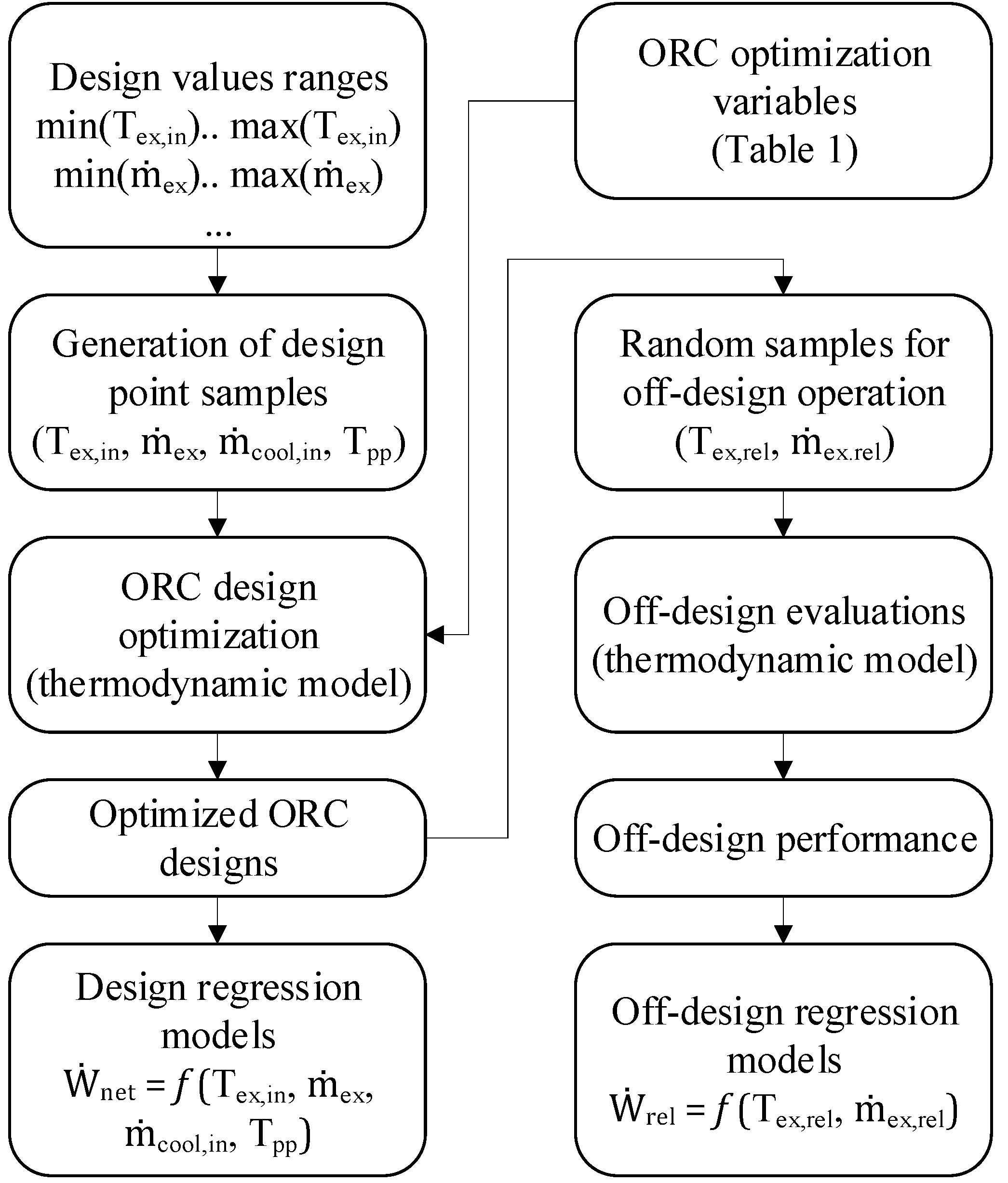
2.3. Data Generation and Regression Models

The regression surfaces for the estimation of the ORC design point power output were obtained by fitting the results of a dataset attained by running 200 independent ORC design optimizations, based on random design parameters. Two regression surfaces were attained:

• Design regression model #1, where the sampled parameters were the heat source inlet temperature and mass flow rate, as well as the cooling water inlet temperature.
• Design regression model #2, where also the boiler and condenser pinch point temperatures (ΔT_pp,boil and ΔT_pp,cond) were included as sampled parameters in the optimization routines.

In both cases, the samples of the ORC design parameters were generated using the Sobol method [35] to ensure a good coverage of the sampling space, and the sampled parameters were constrained to be within the boundaries described in Table 2. Only the samples leading to ORC units with a power output in the range 250 kW to 2500 kW were considered in the regression procedure, and this ensured that the accuracy of the attained regression curves was not affected by the presence of outliers.

With respect to the boundaries defined for the heat source temperature, mass flow rate, and the cooling water temperature, a comparison with data retrieved from the MAN Energy Solutions CEAS calculation tool [36], suggests that the engine waste heat characteristics are within the considered ranges, when considering engines in the range from 5 MW to 50 MW operating with different tuning techniques and sailing both in cold and warm waters.

The off-design performance of every optimized ORC configuration was evaluated in 20 different and randomly generated off-design conditions. Each half of the randomly generated off-design points were imposed a temperature of the exhaust gases higher and lower than the design point, respectively. The exhaust gas mass flow rate was varied within 25% to 100% of the ORC design mass flow rate. The heat source temperature was allowed a deviation of +/- 80 °C compared to the design value. The sea water temperature was kept constant in all the off-design simulations.

A single regression model was attained for the characterization of the ORC off-design performance, considering an ORC load ranging for 10% to 100%, and based on the ORC designs used for both design models (fixed and variable pinch point temperatures).

Figure 3 provides a graphical overview of the procedure used to derive the regression models. The symbols included in the sketch are explained in Section 3.1 (T_pp refers both to the condenser and boiler pinch point temperature).

The statistical robustness of a regression curve is ensured if the residuals follow a normal distribution and their mean is equal to zero. In addition, there should be no correlation between the residuals themselves and the parameters used to build the regression curve, nor the data points that are being estimated (the ORC net power output and its off-design performance). The validity of the mentioned aspects for the proposed regression surface models was checked with the scatter plots shown in the following sections.

2.4. Case Studies and Optimization Approach

The accuracy of the proposed regression surface models was checked in two test cases. The first case study considers the installation of an ORC unit on board an LNG-fueled feeder ship powered by a 10.5 MW MAN 7S60E-C10.5-GI engine with low pressure selective catalytic reactor tuning. In the second case study, an ORC unit on board a medium size LNG-fueled container vessel powered by a 23 MW MAN 6S80ME-C9.5-GI engine with part-load tuning was considered. The two vessels were assumed to operate according to the load profiles shown in Figure 4, for 4380 and 6500 hours annually, respectively.

These are typical data for the two considered types of vessels. Sea water temperatures of 10 °C, 15 °C, and 20 °C were considered for the case studies.

Table 3. Characteristics of the exhaust gases of the two engines as a function of the engine load [36].

	MAN 7S60E-C10.5-GI		MAN 6S80ME-C9.5-GI
Engine Load (%)	Mass Flow Rate (kg/s)	Temperature (°C)	Mass Flow Rate (kg/s)	Temperature (°C)
100	22.5	251	52	251
90	19	266	47	239
80	18.2	245	44.9	207
70	16.3	243	40.3	206
60	14.3	248	35.7	211
50	12.1	258	30.6	221
40	9.9	271	25	239
30	7.5	280	22.7	205

reports the exhaust mass flow rate and temperature for the two engines as a function of the load. The data was retrieved from the MAN CEAS engine calculation tool [36].

The ORC maximum annual energy production and minimum LCOE required to produce the electricity by means of the ORC unit, were computed both using thermodynamic model and regression model. Both the thermodynamic calculations and the estimations using the regression models were carried out following the procedure shown in Figure 5.

When using the thermodynamic model, the ORC design parameters and design point were selected as optimization parameters, while only the latter was optimized when using the simplified approach based on the regression curves. For the estimation of the accuracy of the regression model #2, three alternative pinch point temperature combinations were considered: (i) ΔT_pp,boil = 25 °C and ΔT_pp,cond = 10 °C, (ii) ΔT_pp,boil = 20 °C and ΔT_pp,cond = 8 °C, and (iii) ΔT_pp,boil = 15 °C and ΔT_pp,cond = 5 °C.

3. Results

This section presents the results obtained throughout the study. First, the set of regression equations is presented. Second, the results of the estimations of model #1 (fixed pinch point values) and thermodynamic models are compared. Third, the comparison focuses on model #2 (variable pinch point values) and the thermodynamic evaluations. Both comparisons analyze the ORC annual energy production and LCOE.

3.1. Regression Models

The fitted regression models to estimate the ORC design power output are given in Equation (4) and Equation (5), for model #1 and model #2, respectively. Note that the pinch point temperature differences are included as parameters in Equation (5). Equation (6) displays the regression model employed to fit the ORC off-design performance, i.e., extending both models #1 and #2.

$${\dot{W}}_{Net}=a+b·\frac{{\dot{m}}_{ex}·T_{ex,in}}{1000}+c·{\dot{m}}_{ex}·{\frac{\left(T_{ex,in}-T_{cool,in}\right)}{10,000,000}}^3$$

(4)

$$\begin{gathered} {\dot{W}}_{Net}=a+b·\frac{{\dot{m}}_{ex}·T_{ex,in}}{1000}+c·{\dot{m}}_{ex}·{\frac{\left(T_{ex,in}-T_{cool,in}\right)}{10,000,000}}^3+ \\ d·\frac{{\dot{m}}_{ex}·T_{ex,in}·\Delta T_{pp,boil}}{10,000}+e·\frac{{\dot{m}}_{ex}·T_{cool,in}·\Delta T_{pp,cond}}{100}, \end{gathered}$$

(5)

$${\dot{W}}_{rel}=\frac{{\dot{W}}_{off}}{{\dot{W}}_{Net}}=a+b·\sqrt{{\dot{m}}_{ex,rel}}+c·{\dot{m}}_{ex,rel}·T_{ex,rel}^2,$$

(6)

The off-design regression curve estimates the ORC relative net power output (Ẇ_rel) in comparison with the design point conditions. The selected predictors are the relative exhaust gases mass flow rate (ṁ_ex.rel) and temperature (T_ex,rel), defined as follows:

$${\dot{m}}_{ex,rel}=\frac{{\dot{m}}_{ex,off}}{{\dot{m}}_{ex,des}},$$

(7)

$$T_{ex,rel }= \frac{T_{ex,in,off }}{T_{ex,in,des }},$$

(8)

where the subscripts ‘des’ and ‘off’ refer to design and off-design conditions, respectively.

Table 4. Regression coefficients and standard errors of the proposed regression models.

	Design Model #1		Design Model #2		Off-Design Model
	Value	Standard Error	Value	Standard Error	Value	Standard Error
a	11.2332	5.5082	11.6575	5.7680	−0.1372	0.0021
b	10.0910	0.5773	39.6980	1.3410	0.1420	0.0035
c	19.2098	0.1247	18.3483	0.1411	1.0439	0.0022
d	-	-	−10.6565	0.4166	-	-
e	-	-	−0.6786	0.0687	-	-

shows the regression coefficients and standard errors for the two proposed regression curves. The standard errors of each of the coefficients are smaller than the coefficient themselves, suggesting that all the coefficients were identified with high accuracy. The ‘a’ coefficients for design model #1 and #2 have relatively high standard error compared to the other parameters. The corresponding P-values are equal to 0.043 (model #1) and 0.045 (model #2). The P-values represent the result of the P-test aiming at understanding whether a regression parameter is significant to the prediction. Given that all the P-values are below 0.05, it can be concluded that all the selected parameters are highly significant (as should be expected).

Table 5. Statistical parameters of the proposed regression models.

Equation	Adjusted R2	Standard Error	F-Significance	Average Rel. Error (%)
Design model #1	0.9979	27.44 kW	2.2 × 10−180	1.94
Design model #2	0.9978	29.09 kW	3.5 × 10−179	1.76
Off-design model	0.9881	0.0251 (-)	0	4.61

shows the adjusted R² value, standard error, and average relative error in the prediction for the proposed regression curves. For both equations, the R² value approaches unity, while the average error is within 4.61%. The F-significances of all the models approach zero.

For the three regression models, the mean of the residuals is below 1 × 10⁻¹³, hence validating the assumption that the mean of the residuals is close to zero. In addition, the residuals appeared to follow a normal distribution, except for the presence of some tails (see Figure 6). The computed R² obtained with a straight trend line are 89.7%, 92.7%, and 96.1%, for the three models, respectively.

Figure 7, Figure 8 and Figure 9 show the scatter plots of the regression’s standard residuals as a function of the prediction and the regression parameters (predictors). The plots indicate that the homoscedasticity assumption (the variance of the residuals should not vary as a function of the predicted value, nor the predictor) can be considered acceptable for the off-design regression curve (Figure 9), but is possibly not valid/less convincing in the case of the design point regression models (Figure 7 and Figure 8).

The figures indicate that the spread of the residuals increases, for example, as the predicted ORC net power output increases. A further analysis of the residuals suggests that the absolute error in the prediction increases as a function of the ORC net power output, while the relative deviation remains mostly constant. According to the indications from Gujarati and Porter [37], a violation of the homoscedasticity assumption does not lead to the attainment of biased regression parameters, but rather to an inaccurate estimation of the standard errors of such parameters.

Figure 10 depicts the predicted values against the data used for the regression for the two cases and illustrates the fit between data and predictions. The design point models appear to predict the thermodynamic model in a very accurate way, while there is a larger spread of the results in the off-design model, due to the complexity of the phenomena taking place during off-design operation of the unit.

3.2. Comparison with the Thermodynamic Evaluations (Model #1—fixed pinch points)

The results of the overall ORC optimization using the thermodynamic simulation model and the regression curves (model #1) are shown in

Table 6. Comparison between the solutions attained using the thermodynamic models and the regression curves (model #1): energy production maximization cases.

	Thermodynamic Models	Regression Curves	Difference (%)
Feeder (Tsw = 10 °C)
ORC design load (%)	90	90.0	0.00
ORC design power (kW)	658.7	674.6	2.41
ORC annual production (MWh)	2246	2326	3.56
LCOE ($/kWh)	0.092	0.090	−1.75
Feeder (Tsw = 15 °C)
ORC design load (%)	90	90.0	0.00
ORC design power (kW)	621.8	639.4	2.83
ORC annual production (MWh)	2115	2205	4.21
LCOE ($/kWh)	0.093	0.091	−2.04
Feeder (Tsw = 20 °C)
ORC design load (%)	90	90.0	0.00
ORC design power (kW)	586.6	605.6	3.24
ORC annual production (MWh)	1989	2088	4.97
LCOE ($/kWh)	0.095	0.093	−2.53
Container vessel (Tsw = 10 °C)
ORC design load (%)	100	100.0	0.00
ORC design power (kW)	1500.7	1538.2	2.50
ORC annual production (MWh)	4648	4419	−4.93
LCOE ($/kWh)	0.081	0.086	7.06
Container vessel (Tsw = 15 °C)
ORC design load (%)	100	100.0	0.00
ORC design power (kW)	1409.4	1453.2	3.11
ORC annual production (MWh)	4333	4175	−3.65
LCOE ($/kWh)	0.083	0.088	6.05
Container vessel (Tsw = 20 °C)
ORC design load (%)	100	100.0	0.00
ORC design power (kW)	1323	1372	3.68
ORC annual production (MWh)	4031	3941	−2.22
LCOE ($/kWh)	0.085	0.089	4.95

and

Table 7. Comparison between the solutions attained using the thermodynamic models and the regression curves (model #1): energy production maximization cases.

	Thermodynamic Models	Regression Curves	Difference (%)
Feeder (Tsw = 10 °C)
ORC design load (%)	75	78.4	4.47
ORC design power (kW)	458.2	498.0	8.69
ORC annual production (MWh)	1843	1979	7.40
LCOE ($/kWh)	0.086	0.085	−1.05
Feeder (Tsw = 15 °C)
ORC design load (%)	75	78.4	4.48
ORC design power (kW)	430.7	470.3	9.20
ORC annual production (MWh)	1732	1869	7.93
LCOE ($/kWh)	0.087	0.086	−1.15
Feeder (Tsw = 20 °C)
ORC design load (%)	75	78.4	4.47
ORC design power (kW)	404.2	443.7	9.76
ORC annual production (MWh)	1625	1763	8.53
LCOE ($/kWh)	0.089	0.087	−1.80
Container vessel (Tsw = 10 °C)
ORC design load (%)	37.45	35.0	−6.54
ORC design power (kW)	633.9	631.5	−0.38
ORC annual production (MWh)	3831	3823	−0.20
LCOE ($/kWh)	0.0522	0.0522	0.00
Container vessel (Tsw = 15 °C)
ORC design load (%)	35.73	35.0	−2.05
ORC design power (kW)	587.7	596.5	1.49
ORC annual production (MWh)	3560	3611	1.44
LCOE ($/kWh)	0.053	0.053	−0.38
Container vessel (Tsw = 20 °C)
ORC design load (%)	35	35.0	0.00
ORC design power (kW)	547.8	562.9	2.76
ORC annual production (MWh)	3318	3408	2.70
LCOE ($/kWh)	0.0542	0.054	−0.74

. The results indicate that the simplified approach based on the regression model #1 accurately predicts the optimal design and economic performance of the ORC unit on board the two considered vessels. The maximum deviations are 6.54%, 9.76%, 8.53%, and 6.05% for the ORC design point, ORC design power output, annual production, and LCOE, respectively.

From the perspective of the computational time, the thermodynamic optimization requires around 1 hour of simulation time, while the simplified approach requires less than 1 second. The ORC evaporation temperatures were found to be in the range from 137.6 to 160.8 °C, while the ORC condensation temperature were in the range from 22.4 to 32.4 °C.

Figure 11 shows the computed ORC power production as a function of the main engine load for the considered cases.

Even in this case, the regression models are proven to be capable of accurately reproducing the part load operation of the optimized ORC units along the various engine loads. The greatest deviations appear in Figure 10c (feeder optimized for minimum LCOE), where the ORC power production is slightly overestimated when the engine is operated at loads above 60%. This is due to an overestimation of the ORC design point, which is found to be at an engine load of 75% in the thermodynamic simulations, and at an engine load of 78.4% when using the regression models.

Regarding the optimal design of ORC units, finally, it emerges that units that are optimized to minimize the LCOE are designed for lower engine loads, compared to units that are optimized to maximize the overall energy production. In particular, the design load that minimizes the system LCOE is of 75% and 35% for the feeder and the container vessel, respectively. Designing the unit for a lower engine load ensures that the ORC is operated in the design point for a higher amount of time, and hence a lower cost of the produced energy, compared to when the unit is mostly operated in part-load conditions, with lower conversion efficiencies.

3.3. Comparison with the Thermodynamic Evaluations (Model #2—variable pinch points)

Table 8. Comparison between the solutions attained using the thermodynamic models and the regression curves (model #2): energy production maximization cases.

	Thermodynamic Models	Regression Curves	Difference (%)
Feeder (ΔTpp,boil = 25 °C; ΔTpp,cond = 10 °C)
ORC design load (%)	90.0	90.0	0.0
ORC design power (kW)	575.2	609.5	6.0
ORC annual production (MWh)	1961	2102	7.2
LCOE ($/kWh)	0.095	0.093	−2.6
Feeder (ΔTpp,boil = 20 °C; ΔTpp,cond = 8 °C)
ORC design load (%)	90.0	90.0	0.00
ORC design power (kW)	621.8	640.4	2.98
ORC annual production (MWh)	2115	2208	4.37
LCOE ($/kWh)	0.093	0.091	−2.15
Feeder (ΔTpp,boil = 15 °C; ΔTpp,cond = 5 °C)
ORC design load (%)	90.0	90.0	0.00
ORC design power (kW)	678.9	673.1	−0.85
ORC annual production (MWh)	2300	2321	0.90
LCOE ($/kWh)	0.091	0.090	−1.53
Container vessel (ΔTpp,boil = 25 °C; ΔTpp,cond = 10 °C)
ORC design load (%)	100.0	100.0	0.00
ORC design power (kW)	1300.0	1380.6	6.20
ORC annual production (MWh)	4050	3996	−1.32
LCOE ($/kWh)	0.083	0.089	6.71
Container vessel (ΔTpp,boil = 20 °C; ΔTpp,cond = 8 °C)
ORC design load (%)	100.0	100.0	0.00
ORC design power (kW)	1409.4	1460.6	3.63
ORC annual production (MWh)	4333	4196	−3.15
LCOE ($/kWh)	0.083	0.088	5.93
Container vessel (ΔTpp,boil = 15 °C; ΔTpp,cond = 5 °C)
ORC design load (%)	100.0	100.0	0.00
ORC design power (kW)	1542.0	1545.9	0.25
ORC annual production (MWh)	4656	4441	−4.62
LCOE ($/kWh)	0.082	0.086	4.99

and

Table 9. Comparison between the solutions attained using the thermodynamic models and the regression curves (model #2): LCOE minimization cases.

	Thermodynamic Models	Regression Curves	Difference (%)
Feeder (ΔTpp,boil = 25 °C; ΔTpp,cond = 10 °C)
ORC design load (%)	75.0	78.4	4.28
ORC design power (kW)	397.1	446.9	11.14
ORC annual production (MWh)	1598	1776	10.01
LCOE ($/kWh)	0.089	0.087	−1.95
Feeder (ΔTpp,boil = 20 °C; ΔTpp,cond = 8 °C)
ORC design load (%)	75.0	78.4	4.47
ORC design power (kW)	430.7	473.8	10.02
ORC annual production (MWh)	1732	1883	8.74
LCOE ($/kWh)	0.087	0.086	−1.38
Feeder (ΔTpp,boil = 15 °C; ΔTpp,cond = 5 °C)
ORC design load (%)	75.0	78.4	4.47
ORC design power (kW)	474.3	502.6	5.95
ORC annual production (MWh)	1902	1997	5.02
LCOE ($/kWh)	0.085	0.085	−0.71
Container vessel (ΔTpp,boil = 25 °C; ΔTpp,cond = 10 °C)
ORC design load (%)	35.5	35.0	−1.39
ORC design power (kW)	539.8	566.8	4.77
ORC annual production (MWh)	3273	3431	4.63
LCOE ($/kWh)	0.054	0.054	−1.12
Container vessel (ΔTpp,boil = 20 °C; ΔTpp,cond = 8 °C)
ORC design load (%)	35.7	35.0	−2.05
ORC design power (kW)	587.7	600.4	2.15
ORC annual production (MWh)	3560	3635	2.11
LCOE ($/kWh)	0.053	0.053	−0.56
Container vessel (ΔTpp,boil = 15 °C; ΔTpp,cond = 5 °C)
ORC design load (%)	36.5	35.0	−4.26
ORC design power (kW)	649.2	636.3	−2.03
ORC annual production (MWh)	3922	3852	−1.81
LCOE ($/kWh)	0.052	0.052	0.38

show the results of the overall ORC optimizations using the thermodynamic simulation tool and the regression model #2. In all cases, a sea water temperature of 15 °C was assumed. Table 8 displays the solutions attained when maximizing the ORC annual energy production, while Table 9 depicts the results attained when minimizing the LCOE of the system. Different cases were considered, where the minimum pinch points temperatures both in the boiler and the condenser are varied. This allows to check the suitability of the regression model #2 to capture the impact of the minimum pinch point temperatures on the attainable performance of the unit. The results suggest that the maximum deviations for the engine load for which the ORC should be designed, ORC design power output, annual production, and LCOE, are 4.47%, 11.14%, 10.01%, and 6.71%. As it could be expected, the inclusion of more model parameters, namely the pinch points, decreases the accuracy of the estimations. The average deviations in the estimated annual productions and LCOE are 4.48% and 2.5%, indicating that even regression model #2 is suitable to carry out preliminary estimations for the optimal design and performance of ORC units to be installed on board ships using low-sulfur fuels.

It emerges that the optimal design load of the engine for which the ORC should be designed is not affected by the selected pinch point values. Additionally, as expected, a decrease in the pinch points is connected with an increase of the annual energy production from the ORC. The ORC production curves as a function of the engine load are not reported for this case, because a comparison between the results attained using model #1 and model #2 for the case where the pinch points are set to 20 °C (for the boiler) and 8 °C (for the condenser), indicated that the power production curves given by the two regression models are overlapping. The ORC evaporation temperatures were found to be in the range from 137.5 to 162.4 °C, while the ORC condensation temperatures were in the range from 24.4 to 29.5 °C.

4. Discussion

The procedure followed to derive the proposed regression curves is typical of the data-driven modelling approach, which is now gaining interest due to the increasing data availability and the development of more and more sophisticated machine-learning algorithms. The proposed algorithms are attained by implementing a supervised machine learning approach, where both the model outputs (i.e., the ORC power output) and the model input (i.e., the characteristics of the main engine exhaust gases) are known.

A more rigorous implementation of the data-driven modelling approach to derive the regression curves would have required to split the available dataset into training and test sets. This is because regression algorithms are generally developed based on a portion of the overall data (train set), and then their accuracy is tested on the remaining portion of the data (test set). This allows to prove the reliability of the proposed algorithm to predict the model output also for data outside the space covered by the data used for its development.

This was considered not to be required for our case, because the accuracy of the proposed approach, which combines design and off-design regression models, was verified through several case studies, whose inputs parameters were not used when generating the regression curves.

In any case, the authors do not recommend the use of the proposed regression models when using such curves outside their validation space (i.e., increased temperatures of the exhaust gases, or reduced flow rates).

In addition, as a way to reduce the model complexity, several assumptions were made which could influence the attained results. In particular, the evaluations were limited to one fluid, the backpressure effect on the engine was neglected, and the pressure drops in the heat exchangers were not accounted for. The decision not to consider the impact on the backpressure effect was mainly connected to two reasons: (1) the findings from Michos et al. [14] indicated that such parameter has a weak impact on the overall estimated savings, and (2) the acceptable backpressure level to the engine varies both with the selected engine and the considered engine load, making it a complex feature to include in simplified regression models.

With respect to the approach used to estimate the cost of the unit, it should be mentioned that large uncertainties are expected, because the cost of the unit is not uniquely identified by its overall size, but is influenced also by other parameters, such as the operating pressures, the selected materials, and the configuration of the installation in the engine system. The attained economic results are therefore to be considered as preliminary and are meant to give a first estimate.

5. Conclusions

This paper presented an accurate and time-efficient method to estimate the techno-economic prospects for organic Rankine cycle-based waste heat recovery units tailored for ships using low-sulfur fuels. The proposed method is derived by integrating regression curves capable of describing the design and off-design performance of organic Rankine cycle units. The user-specified input parameters are the temperature and mass flow rate of the ship’s exhaust gases, as well as the ship sailing profile. Both the statistical significance and the expected accuracy of the proposed regression curves were analyzed. In comparison with the evaluations carried out using standard thermodynamic-based models, maximum deviations of 8.53% and 6.05% in the estimated organic Rankine cycle annual energy production and levelized cost of electricity were attained when considering the regression model #1 (fixed ORC pinch points). The deviations increased to 10% for the annual energy production, and 6.7% for the levelized cost of electricity for the regression model #2, when the unit’s pinch points were included as parameters in the regression curves. The proposed method assumes that the organic Rankine cycle that maximizes the net power production in design conditions is the one resulting in the greatest energy production on an annual basis. The comparison between the regression models and the thermodynamic evaluations, which did not include this premise, demonstrated that this assumption does not significantly affect the accuracy of the estimations.

The proposed method is simple, leads to accurate estimations, and is characterized by a short computational time (less than one second). This makes it suitable to be used for preliminary evaluations of the potential for installing organic Rankine cycle power systems on board a wide range of vessel types. In addition, the proposed approach can be used even by non-experts in the organic Rankine cycle technology, and hence it can be of interest for a wide audience of readers.

References

1. Nitrogen Oxides (NOx) Regulation 13; Tech. Rep.; International Maritime Organization: London, UK, 2015.
2. Sulfur Oxides (SOx) Regulation 14; Tech. Rep.; International Maritime Organization: London, UK, 2015.
3. The International Maritime Organization. Adoption of the Initial IMO Strategy on Reduction of GHG Emissions from Ships and Existing IMO Activity Related to Reducing GHG Emissions in the Shipping Sector; Tech Rep; International Maritime Organization: London, UK, 2018. [Google Scholar]
4. Brynolf, S.; Fridell, E.; Andersson, K. Environmental assessment of marine fuels: Liquefied natural gas, liquefied biogas, methanol and bio-methanol. J. Clean. Prod. 2014, 74, 86–95. [Google Scholar] [CrossRef]
5. Smith, A.B. Gas fuelled ships: Fundamentals, benefits classification & operational issues. In Proceedings of the 1st Gas Fuelled Conference, Hamburg, Germany, 21 October 2010. [Google Scholar]
6. Bouman, E.A.; Lindstad, E.; Rialland, A.I.; Strømman, A.H. State-of-the-art technologies, measures, and potential for reducing GHG emissions from shipping—A review. Transp. Res. Part D 2017, 52, 408–421. [Google Scholar] [CrossRef]
7. Baldi, F.; Ahlgren, F.; Nguyen, T.; Thern, M.; Andersson, K. Energy and exergy analysis of a cruise ship. Energies 2018, 11, 1–41. [Google Scholar] [CrossRef] [Green Version]
8. Baldi, F.; Nguyen, T.; Ahlgren, F. The application of process integration to the optimisation of cruise ship energy systems: A case study In a context of demand for increased energy efficiency in shipping, this article proposes an example. In Proceedings of the ECOS 2016: 29th International Conference on Efficiency, Cost, Optimization, Simulationand Envirionmental Impact of Energy Systems, Portoroz, Slovenia, 19–23 June 2016. [Google Scholar]
9. Mondejar, M.E.; Andreasen, J.G.; Pierobon, L.; Larsen, U.; Thern, M.; Haglind, F. A review on the use of organic Rankine cycle power systems for marine applications. Renew. Sustain. Energy Rev. 2018, 91, 126–151. [Google Scholar] [CrossRef]
10. Larsen, U.; Sigthorsson, O.; Haglind, F. A comparison of advanced heat recovery power cycles in a combined cycle for large ships. Energy 2014, 74, 260–268. [Google Scholar] [CrossRef] [Green Version]
11. Andreasen, J.G.; Meroni, A.; Haglind, F. A comparison of organic and steam Rankine cycle power systems for waste heat recovery on large ships. Energies 2017, 10, 1–23. [Google Scholar] [CrossRef] [Green Version]
12. Soffiato, M.; Frangopoulos, C.A.; Manente, G.; Rech, S.; Lazzaretto, A. Design optimization of ORC systems for waste heat recovery on board a LNG carrier. Energy Convers. Manag. 2015, 92, 523–534. [Google Scholar] [CrossRef]
13. Baldi, F.; Larsen, U.; Gabrielii, C. Comparison of different procedures for the optimisation of a combined Diesel engine and organic Rankine cycle system based on ship operational profile. Ocean Eng. 2015, 110, 85–93. [Google Scholar] [CrossRef] [Green Version]
14. Michos, C.N.; Lion, S.; Vlaskos, I.; Taccani, R. Analysis of the backpressure effect of an Organic Rankine Cycle (ORC) evaporator on the exhaust line of a turbocharged heavy duty diesel power generator for marine applications. Energy Convers. Manag. 2017, 132, 347–360. [Google Scholar] [CrossRef]
15. Baldasso, E.; Andreasen, J.G.; Mondejar, M.E.; Larsen, U.; Haglind, F. Technical and economic feasibility of organic Rankine cycle-based waste heat recovery systems on feeder ships: Impact of nitrogen oxides emission abatement technologies. Energy Convers. Manag. 2019, 183, 577–589. [Google Scholar] [CrossRef]
16. Rech, S.; Zandarin, S.; Lazzaretto, A.; Frangopoulos, C.A. Design and off-design models of single and two-stage ORC systems on board a LNG carrier for the search of the optimal performance and control strategy. Appl. Energy 2017, 204, 221–241. [Google Scholar] [CrossRef]
17. Liu, B.T.; Chien, K.H.; Wang, C.C. Effect of working fluids on organic Rankine cycle for waste heat recovery. Energy 2004, 29, 1207–1217. [Google Scholar] [CrossRef]
18. Kuo, C.R.; Hsu, S.W.; Chang, K.H.; Wang, C.C. Analysis of a 50 kW organic Rankine cycle system. Energy 2011, 36, 5877–5885. [Google Scholar] [CrossRef]
19. Wang, D.; Ling, X.; Peng, H.; Liu, L.; Tao, L.L. Efficiency and optimal performance evaluation of organic Rankine cycle for low grade waste heat power generation. Energy 2013, 50, 343–352. [Google Scholar] [CrossRef]
20. Larsen, U.; Pierobon, L.; Wronski, J.; Haglind, F. Multiple regression models for the prediction of the maximum obtainable thermal ef fi ciency of organic Rankine cycles. Energy 2013, 1–8. [Google Scholar] [CrossRef] [Green Version]
21. Lecompte, S.; Huisseune, H.; van den Broek, M.; De Paepe, M. Methodical thermodynamic analysis and regression models of organic Rankine cycle architectures for waste heat recovery. Energy 2015, 87, 60–76. [Google Scholar] [CrossRef]
22. Palagi, L.; Sciubba, E.; Tocci, L. A neural network approach to the combined multi-objective optimization of the thermodynamic cycle and the radial inflow turbine for Organic Rankine cycle applications. Appl. Energy 2019, 237, 210–226. [Google Scholar] [CrossRef]
23. Dickes, R.; Dumont, O.; Quoilin, S.; Lemort, V. Performance correlations for characterizing the optimal off-design operation of an ORC power system. Energy Procedia 2017, 129, 907–914. [Google Scholar] [CrossRef]
24. Baldasso, E.; Elg, M.; Haglind, F.; Baldi, F. Comparative Analysis of Linear and Non-Linear Programming Techniques for the Optimization of Ship Machinery Systems. J. Mar. Sci. Eng. 2019, 7. [Google Scholar] [CrossRef] [Green Version]
25. Andreasen, J.G.; Larsen, U.; Knudsen, T.; Pierobon, L.; Haglind, F. Selection and optimization of pure and mixed working fluids for low grade heat utilization using organic rankine cycles. Energy 2014, 73, 204–213. [Google Scholar] [CrossRef] [Green Version]
26. Rayegan, R.; Tao, Y.X. A procedure to select working fluids for Solar Organic Rankine Cycles (ORCs). Renew. Energy 2011, 36, 659–670. [Google Scholar] [CrossRef]
27. Drescher, U.; Brüggemann, D. Fluid selection for the Organic Rankine Cycle (ORC) in biomass power and heat plants. Appl. Therm. Eng. 2007, 27, 223–228. [Google Scholar] [CrossRef]
28. MAN Energy Solutions. Waste Heat Recovery Systems (WHRS)—Marine Engines & Systems; Tech. Rep.; MAN Energy Solutions: Copenhagen, Denmark, 2014. [Google Scholar]
29. Bell, I.H.; Wronski, J.; Quoilin, S.; Lemort, V. Pure and pseudo-pure fluid thermophysical property evaluation and the open-source thermophysical property library CoolProp. Ind. Eng. Chem. Res. 2014, 53, 2498–2508. [Google Scholar] [CrossRef] [PubMed] [Green Version]
30. MathWorks Official Website. Available online: https://mathworks.com/products/matlab.html (accessed on 31 January 2018).
31. Haglind, F.; Mondejar, M.E.; Andreasen, J.G.; Pierobon, L.; Meroni, A. Organic Rankine Cycle Unit for Waste Heat Recovery on Ships (PilotORC)—Final Report; Tech. Rep.; Department of Mechanical Engineering, Technical University of Denmark (DTU): Copenhagen, Denmark, 2017. [Google Scholar]
32. Usman, M.; Imran, M.; Yang, Y.; Hyun, D.; Park, B. Thermo-economic comparison of air-cooled and cooling tower based Organic Rankine Cycle (ORC) with R245fa and R1233zde as candidate working fl uids for different geographical climate conditions. Energy 2017, 123, 353–366. [Google Scholar] [CrossRef]
33. Turton, R.; Bailie, R.C.; Whiting, W.B.; Shaeiwitz, J.A.; Bhattacharyya, D. Analysis, Synthesis and Design of Chemical Processes, 3rd ed.; Pearson Education: London, UK, 2013; ISBN 9788578110796. [Google Scholar]
34. Lemmens, S. Cost engineering techniques and their applicability for cost estimation of organic rankine cycle systems. Energies 2016, 9, 485. [Google Scholar] [CrossRef] [Green Version]
35. Sobol, I.M.; Turchaninov, V.; Levitan, Y.L.; Shukhamn, B.V. Quasirandom sequence generators. In Proceedings of the IPM ZAK, no. 30; Keldysh Institute of Applied Mathematics, Russian Academy of Sciences: Moscow, Russia, 1992. [Google Scholar]
36. MAN Energy Solutions CEAS Calculation Tool. Available online: https://marine.man-es.com/two-stroke/ceas (accessed on 12 December 2018).
37. Guijarati, D.N.; Porder, D.C. Basic Econometrics, 6th ed.; McGraw-Hill: Boston, MA, USA,, 2009. [Google Scholar]
Figure 1. Considered organic Rankine cycle (ORC): (a) layout, (b) T-s diagram.
Energies 13 01378 g001
Figure 2. ORC-specific cost as a function of its size. The data was retrieved from Lemmens [34].
Energies 13 01378 g002
Figure 3. Procedure used to derive the ORC performance regression models.
Energies 13 01378 g003
Figure 4. Considered annual engine load profiles: (a) Feeder, (b) Container vessel.
Energies 13 01378 g004
Figure 5. Procedure used to optimize the ORC annual energy production/LCOE: (a) thermodynamic models, (b) regression models.
Energies 13 01378 g005
Figure 6. Normal probability plot of the standard residuals: (a) design regression model #1, (b) design regression model #2, (c) off-design regression model (R = 0.897; 0.960).
Energies 13 01378 g006
Figure 7. Design regression model #1, standard residuals distribution according to the target data and regression parameters.
Energies 13 01378 g007
Figure 8. Design regression model #2, standard residuals distribution according to the target data and regression parameters.
Energies 13 01378 g008
Figure 9. Off-design regression model, standard residuals distribution according to the target data and regression parameters.
Energies 13 01378 g009
Figure 10. Predicted values against regression data: (a) design regression model #1, (b) design regression model #1, (c) off-design regression model.
Energies 13 01378 g010
Figure 11. ORC power output as a function of the engine load estimated by the thermodynamic model and by the regression model #1: (a) feeder—maximization of energy production, (b) container vessel—maximization of energy production, (c) feeder—minimization of LCOE, (d) container vessel—minimization of LCOE.
Energies 13 01378 g011