Abstract
This paper presents several applications of Wien Automatic System Planning (WASP) tool to address specific modeling challenges encountered in power system expansion planning problems. Although WASP has been used by power system planners around the world for many decades, its standard formulation does not allow the user to explicitly model many situations that can occur in realistic power systems. Examples of such situations include dual-fuel plants, options for electricity exports, energy exchange agreements with neighboring systems, and considering large generating units as candidates in relatively small-size systems. A number of alternative modeling solutions are proposed in the paper based on the authors’ long-term experience in carrying out generation expansion studies for electricity systems of various types and sizes. These solutions demonstrate the flexibility of using WASP to model atypical features of power systems.
1. Introduction
The generation expansion planning problem is one of the oldest and most thoroughly studied problems in the electricity industry [1]. Its objective is to determine which generating units should be installed and when over the course of a long-term planning horizon of typically several decades [2,3]. The main objective of the expansion planning problem is to minimize the Net Present Value (NPV) of the total investment and operating cost associated with electricity generation over the planning horizon, while meeting the system demand, reliability criteria [4] and any other user-defined constraints (e.g., fuel availability, emissions from electricity generation etc.) [5].
Electric power system expansion planning is typically a highly constrained, nonlinear and discrete optimization problem. A number of approaches and techniques have been developed over the past several decades to solve this problem [5,6]. Traditionally the most successful approaches have been based on linear programming and dynamic programming [7]. More recently, a number of new emerging techniques have been proposed to solve the generation expansion problem, including genetic algorithms, evolutionary programming, ant colony optimization, particle swarm optimization, tabu search and simulated annealing [8].
Wien Automatic System Planning (WASP) model is a power generation capacity expansion planning tool developed for the International Atomic Energy Agency (IAEA). It has been successfully used for several decades by power system planners around the world. Due to its continuous development and improvement in order to accommodate users’ needs, WASP has become one of the most applied and long-lived models for power system expansion planning studies [9,10].
Since it is impossible to accurately incorporate in the model each and every situation found in real-life power systems, WASP users have been encountering many specific situations where standard modeling features of WASP had to be extended in innovative ways. The key objective of this paper is to propose solutions to modeling challenges through several case studies where the WASP modeling framework was used to adequately represent non-typical system features. These non-standard features included seasonal dual-fuel plants, commercial arrangements for power producers, modeling electricity exchanges between systems, integrating electricity exports and imports into the model and considering large expansion candidates in small-size power systems.
WASP model was originally developed by the Tennessee Valley Authority (TVA) and Oak Ridge National Laboratory (ORNL) of the USA to meet the needs of the IAEA’s Market Survey for Nuclear Power in Developing Countries conducted by the Agency in 1972–1973.
Based on the experience gained in using the program, many improvements were made to the computer code by IAEA staff, which led to versions WASP-II (1976), WASP-III (1980) and WASP-III Plus (1991), all of which have been released to IAEA Member States [9]. In order to meet the needs of electricity planners and following the recommendations that environmental and health impacts of electricity sector should be incorporated into the comparative assessment of various electricity generation options, the most recent version of the model has been released as WASP-IV [10].
WASP is designed to find the economically optimal generation expansion policy for an electric utility system within user-specified constraints. It utilizes the following mathematical tools:
- Probabilistic estimation of system production costs [11], unserved energy cost [12], and reliability [13];
- Linear programming technique for determining optimal dispatch policy [14], satisfying exogenous constraints on environmental emissions, fuel availability and electricity generation by some plants;
- Dynamic method of optimization for comparing the costs of alternative system expansion policies.
The WASP-IV code permits finding the optimal expansion plan for a power generating system over a period of up to thirty years, within constraints given by the planner. The optimum is evaluated in terms of minimum discounted total costs. Each possible sequence of power units added to the system (expansion plan or expansion policy) meeting the constraints is evaluated by means of its Total Cost (TC) as the objective function, which is composed of:
- Capital investment costs (CC),
- Salvage value of investment costs (SV),
- Fuel costs (FC),
- Non-fuel operation and maintenance costs (OMC),
- Cost of the energy not served (ENSC),
and expressed as:
where t is year index and T is the total number of years considered (i.e., the length of planning period).
The optimal expansion plan is determined by finding the acceptable system configuration (i.e., the schedule of adding new units to the system) which results in the lowest total system cost.
Let denote the vector that contains the number of all generating units across all unit types that are in operation in year . It needs to satisfy the following condition:
where represents a vector with the number of units for each type that are known to be starting operation in year (assuming the investment decisions for those units have already been made), specifies the number of units of each type decommissioned in year , and is a vector that contains the number of new units starting operation in year that is subject to optimization.
The model uses dynamic programming optimization to find the least-cost construction schedule for new generating units. It is, therefore, useful to keep the number of possible configurations manageable, so a configuration is only allowed if its installed capacity lies between the specified minimum and maximum reserve margins above the peak demand [15,16], as expressed in the following set of constraints:
where is the system peak demand for year , is the minimum allowed reserve margin, is the total installed capacity of a given configuration in year and is the maximum allowed reserve margin. Both and are expressed relative to peak demand.
Another constraint determining the eligibility of a given configuration is associated with the Loss of Load Probability (LOLP) parameter. It is possible to specify an upper bound in the model, so it only considers those configurations where LOLP meets the following condition:
Dynamic programming is well suited for optimizing sequential decision processes such as those associated with long-term generation expansion planning. Typical computational times, assuming that maximum model capabilities are used (30 years planning period, 12 months per year, five hydro conditions), are in the order of a few minutes, allowing the user to investigate a large number of scenarios in a relatively short time.
2. Description of Modeling Problems and Proposed Solutions
Specific situations where alternative modeling techniques were required and applied will be described through three country case studies. These countries are characterized by rather specific power system features that do not lend themselves easily to standard modeling approaches. Therefore a number of solutions are proposed in this section to overcome these modeling challenges.
2.1. Country Case 1: Mauritius
The Republic of Mauritius is an island country in the southwest Indian Ocean, about 900 kilometers east of Madagascar, with a land area of about 2000 km2 and a population of 1.27 million. It has developed from a low-income, agriculturally based economy to a middle-income diversified economy with growing industrial, financial, and tourist sectors. Sugar cane is grown on about 90% of the cultivated land area and accounts for 25% of export earnings.
Mauritian power system is an island system operated by the Central Electricity Board (CEB). The country possesses no oil, gas or coal reserves, but has renewable resources such as hydro and biomass (mostly as residual products of the sugar cane industry). Available hydro-power capacity on the island has already been almost fully exploited. Non-renewable energy sources used for power generation include imported diesel, coal and gas. The electricity demand has seen a rapid increase due to the expansion of tourism and improvements in living standards.
The sugar industry on Mauritius produces a large volume of bagasse, a biomass residue that remains after sugar cane stalks have been crushed to extract their juice (a typical sugar factory produces nearly 30% of bagasse out of its total crushing). The opportunity was therefore recognized to use this abundant resource to produce electricity and heat (which the industry itself could use). This resulted in a number of Independent Power Producers (IPPs) building power plants throughout the country that use both bagasse and coal as primary fuels, due to the highly seasonal availability of bagasse. Expansion planning tools such as WASP typically do not provide an option to explicitly consider such dual-fuel power plants, which is why an alternative modeling approach was required, as described below.
2.1.1. Problem 1a: Modeling Seasonal Dual-Fuel Plants
Mauritian power generation mix includes many plants that co-fire bagasse and coal for electricity generation. Because of the seasonal nature of the sugar cane harvesting cycle, bagasse is available as fuel only during approximately six months of the year. In the other half of the year, those plants use coal to generate electricity. If the user of the expansion model wants to accurately represent the use of both fuels, such plants cannot be modeled as single units.
2.1.2. Solution 1a: User-Specified Maintenance Schedules
Since WASP does not allow for a direct representation of dual-fuel plants, an alternative approach was adopted where these plants were modeled as two separate thermal units. Figure 1 illustrates this with an example where a dual-fuel power plant TPP Sugar Cube is represented by two separate thermal units: TBAG (using only bagasse during six months of the year) and TCOA (using only coal during the remaining 6 months of the year when bagasse is not available). Since the two units should not be able to produce simultaneously, their maintenance schedules have to be manually set so that the periods when they are available to generally do not overlap.
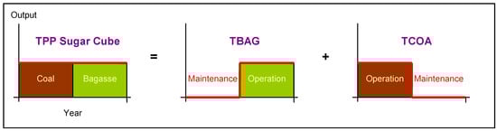
Figure 1.
Representing a dual fuel unit as two thermal units in Wien Automatic System Planning (WASP).
The in-built algorithm for optimizing the plant maintenance schedule in WASP is based on the principle of maintaining sufficient levels of reserve capacity margin over the course of a year. The first step of the algorithm finds the minimum reserve margin for each month :
where is the minimum reserve (in MW) in the system in month , is the available capacity (in MW) in the system in month , and is the peak demand (in MW) in month .
The iterative process then starts by scheduling the maintenance of the largest units during the months with the greatest reserve margin. Once this is determined the new reserve margins are adjusted by discounting the capacity on maintenance. The scheduling algorithm then proceeds by considering the next largest unit type and scheduling its maintenance during months with the greatest adjusted margin. The available headroom for maintenance in month is found as the difference between the minimum margin for that month and the total capacity of generators already selected for maintenance during that month:
where is the available headroom for maintenance (in MW) in month and is the total capacity (in MW) of all units already allocated for maintenance in month . The procedure of adjusting the reserve margins and scheduling unit maintenance continues until all units have their maintenance schedules determined.
The latest release of the WASP model also includes the option for the user to manually specify the maintenance schedule for some or all generating units. The units that do not have their maintenance scheduled by the user are still maintained according to the schedule determined by the model as described above. The user-defined maintenance feature is applied to propose the solution for representing seasonal dual-fuel plants.
The proposed approach to representing the dual-fuel plant as two single-fuel units for this simple case is shown in Figure 1. In actual cases, the duration and starting points of maintenance and operation intervals can vary, but the basic principle remains the same.
The operating windows for the two single-fuel units in this example have been defined so that the units cannot be used simultaneously. This was implemented by using the feature of WASP that allows the user to specify plant maintenance schedules, so that the two units were scheduled to be shut down for maintenance in complementary six-month intervals. The sum of outputs from TBAG and TCOA units adequately represents the total output of TPP Sugar Cube, also allowing for accurate accounting of the consumption of both fuels.
Note that the solution proposed here is only directly applicable for existing dual-fuel plants. If these dual-fuel generators are to be considered as candidates in expansion planning, this would require additional interventions in the model. One possible solution would be to specify the two single-fuel units as candidates for expansion and split the total investment cost of the dual-fuel plant in proportion to the available annual output of both constituent parts, assigning those costs to two single-fuel units. The user would additionally need to iterate the allowed number of new single-fuel units when specifying eligible system configurations in WASP’s CONGEN module, to ensure that the number of both unit subtypes in the cost-optimal solution is equal.
2.1.3. Problem 1b: Modeling IPP Contract Provisions
Many of the dual-fuel (bagasse/coal) power plants were built as IPP projects. They deliver their electricity to the grid based on power purchase agreements (PPAs) between them and the CEB. According to these agreements, the CEB is obliged to purchase a guaranteed share of total plant output (e.g., 80% or 90%). The difficulty in modeling such arrangements in least-cost expansion models is in setting a unit’s annual output to a predefined value given that these result from merit order calculations carried out within the model. WASP-IV does include a possibility to define group limitations, which can also be applied to limiting the annual output for a group of generating unit, but this often yields unwanted results because the program accommodates the group constraint by modifying the loading order of the plants i.e., by pushing the plant(s) included in the constraint towards the end of the loading order.
2.1.4. Solution 1b: User-Specified Loading Order
One option in the MERSIM module of WASP is that the user specifies the loading order of the generating units, instead of the default option that determines the loading order based on variable operating costs. This provides the user with the opportunity to shift a particular unit upwards or downwards in the loading order in order to set its output to the desired level. This procedure is depicted in Figure 2.
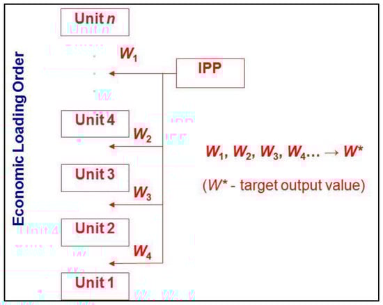
Figure 2.
Adjusting the loading order in order to obtain the desired output value for a unit.
By combining the options to impose group limitations on annual generation and to enforce a user-specified loading order, the user can perform successive model runs and modify the loading order until the desired level of annual output is obtained for a given generating unit.
2.2. Country Case 2: Kosovo
Kosovo is a territory in South–Eastern Europe, defined by the UN resolution 1244 as an autonomous territory within the former Federal Republic of Yugoslavia under UN administration. Its area is around 11,000 km2, and the population is 1.8 million.
Its power system suffered major damages during the violent conflict in 1999, which was exacerbated by poor maintenance of the infrastructure during the 90-ties. This led to many projects being launched from year 2000 onwards by international donors (such as World Bank) in order to improve conditions of power supply in Kosovo. Some of these projects were focused on investigating possibilities to exchange power with the neighboring countries under different arrangements.
2.2.1. Problem 2a: Modeling Different Options for Firm Electricity Exports
Although WASP does offer its users certain possibilities in modeling electricity imports (e.g., by defining a new thermal unit), it does not allow for direct modeling of electricity exports. Since it is a cost-based model, it is not designed to take into account potential revenues from electricity sales outside of the system.
2.2.2. Solution 2a: Recalculating Load Duration Curves for the LOADSY Module
Modeling base power exports for this case was done by modifying the period load duration curves (LDCs). Naturally, this had to be done outside of the model, and then introduced back into the LOADSY module. Figure 3 shows how monthly LDCs change their shape, becoming flatter when fixed baseload exports are calculated into the system load. The user also needs to add fixed base export obligations to the system peak load in years when these exports occur, so that the resulting system load accurately represents the total demand (domestic consumption plus firm exports) that the system is expected to cover.
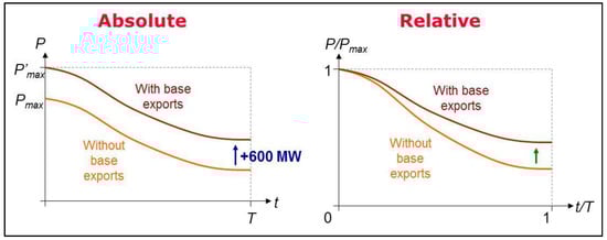
Figure 3.
Modifying absolute and relative load duration curve (LDC) in order to accommodate for base power exports.
In order to evaluate economic performance of different development plans that involve electricity exports, the user needs to assume a price for electricity sales [17], and then, in order to compare this plan to other ‘non-export’ plans, subtract discounted export revenues from the total system cost, which is the objective function minimized by WASP. This calculation needs to be done exogenously, but is relatively straightforward. Such comparison can then indicate which development strategy or scenario seems the most attractive.
2.2.3. Problem 2b: Modeling Various Electricity Exchange Schemes
When studying options for Kosovo’s power system development, it was also necessary to investigate the effect of different electricity exchange schemes with neighboring systems. These regional cooperation schemes can be beneficial to systems such as Kosovo, which are dominated by rather inflexible (lignite-fired) thermal plants. The exchange schemes considered were foreseen as non-commercial arrangements, meaning that the systems trade energy for energy in different ratios without any financial transactions, depending on the conditions of delivery. The exchange schemes considered include:
- Exchanging peak for off-peak energy at a certain ratio (here 2.1)
- Exchanging peak for base-load energy at a certain ratio (here 1.42)
- Exchanging peak/intermediate power for base-load energy at a certain ratio (here 1.1)
2.2.4. Solution 2b: Defining a Pump-Storage Power Plant along with Modifying LDC
As shown in Figure 4, which represents the daily LDC in Kosovo’s power system for a sample day, the daily load diagram is characterized by a considerable difference between the minimum and maximum load, resulting in a relatively low load factor. Importing peak energy contributes to the reduction of system peak load. In return for peak electricity imports, the first co-operation scenario A envisages electricity exports from Kosovo during periods of low demand. The result of such co-operation would be a reconfigured, more convenient daily load duration curve [18] to be met with by the thermal generator portfolio of the Kosovo system, as shown in Figure 4.
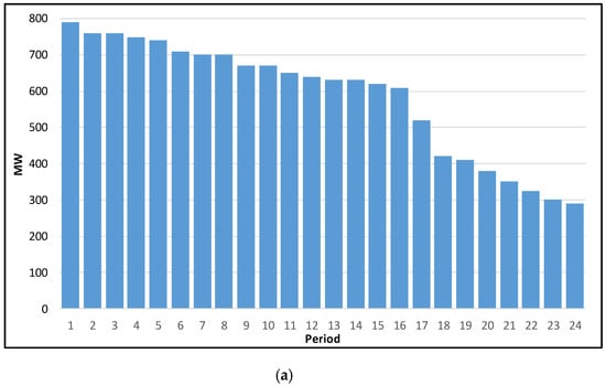
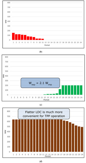
Figure 4.
Alterations in resulting system LDC for scenario A: (a) daily LDC, (b) peak imports, (c) off-peak exports, (d) new LDC.
Simulating such co-operation was implemented in the WASP model by introducing a pumped storage hydro (PSH) power plant [19,20]. Its parameters were set in the way that its capacity in both turbine and pumping mode was made equal (150 MW), while its monthly generation was limited to 20 GWh, and its cycle efficiency was set to 47.6%, which represents the ratio between the volumes of off-peak exports and peak imports (or 1/2.1).
Scenario B also assumed that the peak and intermediate power needed for the Kosovo power system would be ensured by generators in other power systems. For the purpose of compensating the other systems, the Kosovo system should provide them with base-load output. In this case, it was assumed that peak energy imports, with the maximum capacity of 150 MW, would be compensated with the 1.42 times the volume of baseload energy. This arrangement is depicted in Figure 5.
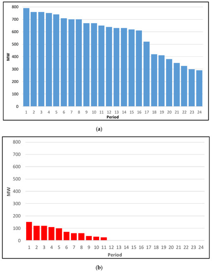
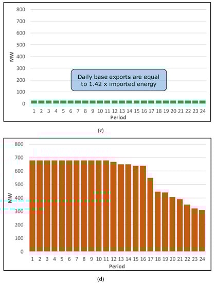
Figure 5.
Alterations in resulting system LDC for scenario B: (a) Daily LDC, (b) peak imports, (c) off-peak exports, (d) new LDC.
The reconfigured LDC is much more suitable for the operation of Kosovo’s inflexible thermal units. This arrangement was simulated in the WASP model by defining a peak (import) unit whose contribution in terms of both power and energy was similar to the import component of scenario A. The annual imported electricity in scenario B was set at the level of the average turbine output of the PSH plant in scenario A. The base-load electricity exports, determined based on the 1.42 factor, were added to the original LDCs. With the annual peak contribution of imported electricity of 152 GWh and a maximum capacity of 150 MW, the electricity base-load export capacity was set at 25 MW.
Finally, scenario C did not foresee any decrease in peak load of the system, with the objective to ensure a more even operation of the existing and planned power plants in Kosovo as well as the possibility of exporting electricity in the base-load. The implications of this scenario are shown in Figure 6.
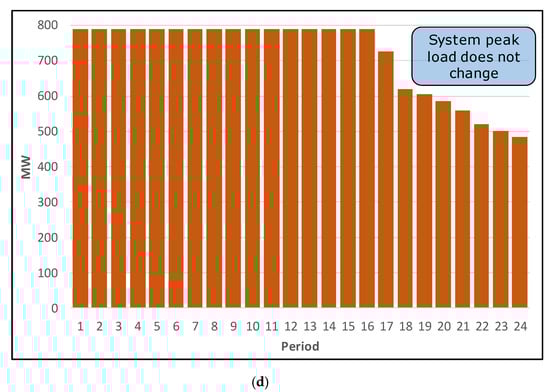
Figure 6.
Alterations in resulting system LDC for scenario C: (a) daily LDC, (b) peak imports, (c) off-peak exports, (d) new LDC.
For this exchange arrangement, the electricity imports to Kosovo deliver up to 200 MW in each time interval. No limitation is imposed on the time for the peak import duration. For the purpose of the counter-exports of electricity from the Kosovo system, 200 MW of electricity base-load is assumed to be available continuously. For this regional co-operation scenario, the overall installed capacity in the Kosovo system is the same as in case of no exchanges with the neighboring systems. On the other hand in scenario C the resulting system demand becomes more evenly distributed, which is much more suitable for the operational characteristics of Kosovo’s generation units.
This scenario of the cross-border co-operation requires the payments for exported and imported electricity to be settled, i.e., to determine the exchange ratio between the electricity exports and imports. The ratio of 1:1.1 was assumed for the transaction-free settlement of the electricity imports against electricity exports. The price that the neighboring systems are willing to pay for any remaining quantity of electricity exported from the Kosovo system within such exchange was assumed at $30/MWh. Within the WASP model, the entire scenario C was implemented through changes in the input LDCs. 200 MW was subtracted from the peak demand hours, while 200 MW were added to the base-load throughout the observed period, taking into account the 1.1 ratio. Accounts of other surpluses in electricity exports were discounted and subtracted from the net present value of total system costs.
2.3. Country Case 3: Montenegro
The Republic of Montenegro is a relatively small country on the Adriatic Sea. Its population of around 650,000 is spread across some 14,000 km2 of the area. Its economy is mainly service-based, with a well-developed tourism industry on the Adriatic coast.
In energy terms, Montenegro possesses some lignite and brown coal resources and a relatively large hydro-power potential, as a result of markedly mountainous terrain. Its power system consists of one coal-fired thermal plant, two large hydro plants, two wind plants, and a few small hydro plants, with total capacity close to 1000 MW. Montenegro relies partly on electricity imports, the main sources of which are Serbia and Bosnia and Herzegovina.
A great number of promising sites for hydro-power plants have been identified in Montenegro so far, but lack of investments, power sector restructuring, incomplete legislative framework and environmental constraints represent the main obstacles for the construction of new facilities.
2.3.1. Problem 3a: Modeling Electricity Exchange for Hydropower Plant Output
One of the two large hydropower plants in Montenegro is HPP Piva with an installed capacity of 342 MW. It follows a specific operating regime stipulated by the long-term contract between the Montenegro power utility (EPCG) and that of neighboring Serbia (EPS). The two utilities have agreed that EPS, being a predominantly thermal system, will dispatch HPP Piva and use its output according to the needs of the Serbian electricity system, and in return supply EPCG with baseload electricity in the amount equal to 1.41 times the expected annual output of HPP Piva. The agreement specifies that EPS will supply 105 MW of base power throughout the entire year (i.e., during 8760 h), as well as additional 105 MW during the two months (usually April and May) when the only thermal power plant in Montenegro, TPP Pljevlja, is shut down for scheduled maintenance.
2.3.2. Solution 3a: Defining Two Thermal Units with Appropriate User-Specified Maintenance Regime
The modeling solution to this problem involved several steps. First, two thermal units were defined: EPS1 and EPS2, Figure 7, both with the maximum capacity of 105 MW. Their variable O&M costs (equivalent to the import prices) were set to zero, in order to position them at the bottom of the merit order, i.e., to ensure that they ‘produce’ with the maximum capacity. Furthermore, for the first plant (EPS1) the duration of scheduled maintenance was set to zero days, while for the second one (EPS2) it was set to 303 days (i.e., 1 year minus 2 months). This maintenance period for EPS2 had to be placed in the correct periods of the year. This was done through user-specified maintenance scheduling available in MERSIM module of WASP, so that 30 days of maintenance have been specified in each month except April and May. Similar to that, the maintenance schedule for TPP Pljevlja was also specified, complementary to the one of EPS2, i.e., covering 60 days of April and May. The procedure is depicted in Figure 7.
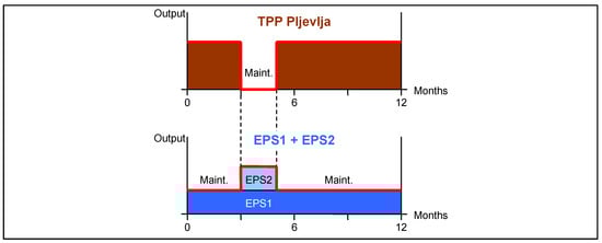
Figure 7.
Specifying maintenance schedules in order to represent base power imports.
This representation of baseload imports allows the model to accurately take into account the realistic operating conditions in the power system of Montenegro. Obviously, since HPP Piva effectively supplies power to another system, and the substituting power is accounted for through specifying EPS1 and EPS2 units, HPP Piva itself was omitted from the description of Montenegro’s power system.
2.3.3. Problem 3b: Candidate Hydro Plant Not Chosen, Despite Lower Cost
As already mentioned, Montenegro has a relatively small power system with a peak demand of around 750 MW. One of the issues with building new hydro-power plants is that many of the proposed projects have rather high installed capacities for a system of that size, exceeding 300 MW, or in some cases even 500 MW. Levelized costs of some of these projects are lower than the competing supply options such as imports. However, because of their size, such plants do not ‘fit’ well into the small system. Economically, their construction is avoided or pushed towards the end of the planning period, because of large investments needed for their construction [21,22,23]. On the other hand, forcing these plants into the system, apart from adding large investment cost to the objective function, is likely to result in energy spillage in some periods of the year, since the system demand is insufficient to absorb such a large amount of energy. This situation is illustrated in Figure 8.
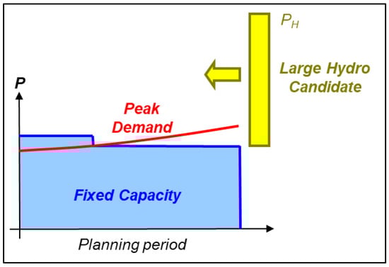
Figure 8.
Large hydro plant candidate in a small power system.
In order to avoid this issue and enable the system to accommodate the large hydro plant, one solution is to adopt an approach similar to the solution to Problem 3a. In other words, one can assume that it is possible to reach an agreement with a neighboring power system in order to share the benefits of a large hydro plant. In this approach, the hydro plant can be represented as an equivalent thermal unit with lower capacity () then the large hydro plant (), as follows in Equation (7):
This approach is illustrated in Figure 9.
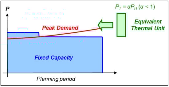
Figure 9.
Modeling a large hydro plant as an equivalent thermal unit.
The problem of fitting a large hydro plant into the LDC of a small system is shown in Figure 10. The capacity factor of the hydro plant in this example is relatively small, but the total capacity after adding the hydro plant (as well as the resulting capacity margin) becomes very high. The annual output of the hydro plant () and the duration curve of its generation are also shown in Figure 10.
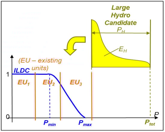
Figure 10.
Fitting a large hydro plant in the LDC.
When representing the large hydro plant as an equivalent thermal unit, in addition to adjusting the capacity of thermal unit according to Equation (8), the available annual output of the thermal unit also should be adjusted (i.e., constrained) as follows:
Coefficients and should be adjusted in line with the conditions in the regional electricity market, or in line with any specific agreements with neighboring power systems. Fitting the annual output of the equivalent thermal unit is shown in Figure 11.
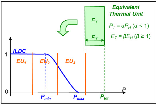
Figure 11.
Fitting the equivalent thermal unit in the LDC.
2.3.4. Solution 3b: Defining Exports Where Possible
There is no straightforward solution to this problem, since the issue arises as the result of the logic of least-cost planning for a single system. Building a large hydro plant with the objective to export its power output requires at least some idea about where that energy is going to be delivered. Otherwise, embarking on such a capital-intensive project would be too risky. If there are any known options for future exports from such a power plant, they can be taken into account by e.g., modifying the system LDCs, analogous to the approach presented for the case of the Kosovo power system.
3. Determining the Sequence of Hydro Candidates in WASP
When introducing hydro-power plants as candidates for future expansion in WASP’s VARSYS module, the user needs to determine their priority list, putting more attractive candidates at the top of the list. Although some flexibility is provided by the possibility to group hydro candidates in WASP in two groups (HYD1 and HYD2), the options for hydro candidates are still limited. In order to evaluate the hydro candidates for the purpose of ordering them in the candidate list, the user, therefore, has to perform additional calculations outside of the model. There are several approaches to this.
The simplest approach is to calculate the so-called investment quotient for each hydro candidate. The investment quotient is obtained by dividing the plant investment cost by the expected annual generation of the plant. For example, if the investment cost of a project is 150 million USD, and the expected annual output of the plant is 300 GWh, the investment quotient is equal to 50 USc/kWh. The calculated investment quotients can then be used to order the candidate hydro plants according to economic attractiveness.
4. Conclusions
This paper suggested several approaches to circumventing certain modeling difficulties in the WASP tool for power system expansion planning, including considering power exports and imports, seasonal dual-fuel plants, IPP contracts etc. These approaches demonstrate how the use of WASP can be extended beyond its standard features, by introducing innovative modeling approaches. This flexibility of WASP to allow its users to work around many modeling challenges has ensured the longevity of the model within the international power system planning community. Future developments of the model will need to take into account the challenges associated with moving towards low-carbon systems, such as the variability of intermittent renewable output and improved modelling of flexible technologies such as energy storage and demand-side response.
Author Contributions
All authors have read and agree to the published version of the manuscript. Conceptualization, M.Z. and M.A.; methodology, G.S.; validation, M.Z. and D.J.; formal analysis, M.Z. and M.A.; investigation, G.S. and D.J.; writing—original draft preparation, M.A.; writing—review and editing, G.S. and D.J.; supervision, M.Z.
Funding
This research received no external funding.
Conflicts of Interest
The authors declare no conflict of interest.
References
- Expansion Planning for Electrical Generating Systems, A Guidebook; International Atomic Energy Agency: Vienna, Austria, 1984.
- Wang, X.; McDonald, J.R. Modern Power System Planning; McGraw-Hill: London, UK, 1994. [Google Scholar]
- Rashidaee, S.A.; Amraee, T.; Fotuhi-Firuzabad, M. A Linear Model for Dynamic Generation Expansion Planning Considering Loss of Load Probability. IEEE Trans. Power Syst. 2018, 33, 6924–6934. [Google Scholar] [CrossRef]
- Park, H.; Baldick, R. Stochastic Generation Capacity Expansion Planning Reducing Greenhouse Gas Emissions. IEEE Trans. Power Syst. 2015, 30, 1026–1034. [Google Scholar] [CrossRef]
- Mehrtash, M.; Kargarian, A. Risk-based dynamic generation and transmission expansion planning with propagating effects of contingencies. Int. J. Electr. Power Energy Syst. 2020, 118, 105762. [Google Scholar] [CrossRef]
- Farhoumandi, M.; Aminifar, F.; Shahidehpour, M. Generation Expansion Planning Considering the Rehabilitation of Aging Generating Units. IEEE Trans. Smart Grid 2020, 1. [Google Scholar] [CrossRef]
- Neelakanta, P.; Arsali, M. Integrated resource planning using segmentation method based dynamic programming. IEEE Trans. Power Syst. 1999, 14, 375–385. [Google Scholar] [CrossRef]
- Zhu, J.; Chow, M.-Y. A review of emerging techniques on generation expansion planning. IEEE Trans. Power Syst. 1997, 12, 1722–1728. [Google Scholar]
- Wien Automatic System Planning (WASP) Package, A Computer Code for Power Generating System Expansion Planning, Version WASP-III Plus, User’s Manual; International Atomic Energy Agency: Vienna, Austria, 1995; Volume 2.
- Wien Automatic System Planning (WASP) Package, A Computer Code for Power Generating System Expansion Planning, Version WASP-IV User’s Manual; International Atomic Energy Agency: Vienna, Austria, 2000.
- Simoglou, C.K.; Bakirtzis, E.A.; Biskas, P.N.; Bakirtzis, A. Probabilistic evaluation of the long-term power system resource adequacy: The Greek case. Energy Policy 2018, 117, 295–306. [Google Scholar] [CrossRef]
- Al-Shaalan, A.M. Reliability evaluation in generation expansion planning based on the expected energy not served. J. King Saud Univ. Eng. Sci. 2012, 24, 11–18. [Google Scholar] [CrossRef]
- Dehghan, S.; Amjady, N.; Conejo, A.J. Reliability-Constrained Robust Power System Expansion Planning. IEEE Trans. Power Syst. 2015, 31, 2383–2392. [Google Scholar] [CrossRef]
- Lauinger, D.; Caliandro, P.; van Herle, J.; Kuhn, D. A linear programming approach to the optimization of residental energy systems. J. Energy Storage 2016, 7, 24–37. [Google Scholar] [CrossRef]
- Zeljko, M. Generation Expansion Planning in the Open Electricity Market. Ph.D. Thesis, Faculty of Electrical Engineering and Computing, Zagreb, Croatia, 2003. [Google Scholar]
- Slipac, G.; Zeljko, M.; Šljivac, D. Importance of Reliability Criterion in Power System Expansion Planning. Energies 2019, 12, 1714. [Google Scholar] [CrossRef]
- Khodaei, A.; Shahidehpour, M.; Wu, L.; Li, Z. Coordination of Short-Term Operation Constraints in Multi-Area Expansion Planning. IEEE Trans. Power Syst. 2012, 27, 2242–2250. [Google Scholar] [CrossRef]
- Kloess, M.; Zach, K. Bulk electricity storage technologies for load-leveling operation—An economic assessment for the Austrian and German power market. Electr. Power Energy Syst. 2014, 59, 111–122. [Google Scholar] [CrossRef]
- Barbour, E.; Wilson, I.; Radcliffe, J.; Ding, Y.; Li, Y. A review of pumped hydro energy storage development in significant international electricity markets. Renew. Sustain. Energy Rev. 2016, 61, 421–432. [Google Scholar] [CrossRef]
- Steffen, B. Prospects for Pumped-Hydro Storage in Germany. SSRN Electron. J. 2011, 45, 420–429. [Google Scholar] [CrossRef][Green Version]
- IRENA (International Renewable Energy Agency). Renewable Energy Technologies: Cost Analysis Series (Hydropower); Working Paper, Volume 1: Power Sector Issue 3/5; IRENA: Abu Dhabi, United Arab Emirates, 2012. [Google Scholar]
- IRENA (International Renewable Energy Agency). Volume 1: Power Sector, Issue 4/5, Renewable Energy Technologies: Cost Analysis; IRENA: Abu Dhabi, United Arab Emirates, 2012. [Google Scholar]
- EIA (U.S. Energy Information Administration). Capital Cost Estimates for Utility Scale Electricity Generating Plants. November 2016. Available online: https://www.eia.gov/analysis/studies/powerplants/capitalcost/pdf/capcost_assumption.pdf (accessed on 3 July 2018).
© 2020 by the authors. Licensee MDPI, Basel, Switzerland. This article is an open access article distributed under the terms and conditions of the Creative Commons Attribution (CC BY) license (http://creativecommons.org/licenses/by/4.0/).