Abstract
Since the early stages of the Internet-of-Things (IoT), one of the application scenarios that have been affected the most by this new paradigm is mobility. Smart Cities have greatly benefited from the awareness of some people’s habits to develop efficient mobility services. In particular, knowing how people use public transportation services and move throughout urban infrastructure is crucial in several areas, among which the most prominent are tourism and transportation. Indeed, especially for Public Transportation Companies (PTCs), long- and short-term planning of the transit network requires having a thorough knowledge of the flows of passengers in and out vehicles. Thanks to the ubiquitous presence of Internet connections, this knowledge can be easily enabled by sensors deployed on board of public transport vehicles. In this paper, a Wi-Fi-based Automatic Bus pAssenger CoUnting System, named iABACUS, is presented. The objective of iABACUS is to observe and analyze urban mobility by tracking passengers throughout their journey on public transportation vehicles, without the need for them to take any action. Test results proves that iABACUS efficiently detects the number of devices with an active Wi-Fi interface, with an accuracy of 100% in the static case and almost 94% in the dynamic case. In the latter case, there is a random error that only appears when two bus stops are very close to each other.
1. Introduction
Urban mobility and flow of people throughout urban infrastructures have a great impact on several areas, such as tourism and transportation [1,2]. In particular, being able to accurately count the number of passengers represents one of the most relevant components of the transit service, since it provides a key measure of the effectiveness of Public Transportation Companies (PTCs) and is pivotal for the efficient planning of the transit network, both in the long and short term [3,4]. Indeed, long-term planning of routes and related timetables is enabled through the analysis of origin–destination matrices, which provide information on commuting flows. Moreover, such matrices give indications regarding the congested time and routes, which simplify short term planning strategies as well, e.g., through the re-assignment of buses to a specific route. Thus, long- and short-term planning contributes to the efficient use of resources and guarantees that buses run where and when passengers need them [5].
To obtain information regarding passenger volumes, PTCs have typically employed traditional mechanisms, going from non-automatic human visual counting, to Automatic Passenger Counting (APC) methods based on various data acquisition technologies (e.g., mat sensors [6], infrared sensors [7], video cameras [8]). These systems require to be installed on vehicles, and are usually quite expensive. With the advent of the Internet of Things (IoT), APC Systems (APCS) has seen a huge boost in the development of new methods to “observe" urban mobility, particularly in recent years. Nevertheless, the great success of recent APCS is primarily due to the advent of portable and mobile devices such as tablets, smartphones and smartwatches, which give new opportunities to collect detailed passengers’ data and to track their movements throughout the cities [9,10]. However, so far, the research in this direction has been mainly focused on determining the travel mode from data collected by various sensors, such as accelerometers and Global Positioning System/Geographycal Information System (GPS/GIS) [11,12]. Furthermore, most of these approaches require that passengers have a specific smartphone app installed on their devices. Therefore, results severely depend on the willingness of passengers to participate. This is not compatible with APCS, which rely on crowd counting principles.
Only recently, Wi-Fi has been used to count the number of active interfaces detected nearby Wi-Fi Access Points (APs) [13]. These systems are typically based on the identification of the Media Access Control (MAC) address that is associated with a Wi-Fi interface. Examples of such systems are represented by the Amsterdam Airport Schiphol [14] and Transport for London (TfL) stations [15]. However, they can effectively work only for obsolete operating systems (earlier than Android 5.0, iOS 7 and Windows Phone 8). In fact, with the aim to protect their users’ privacy against device tracking, Google, Apple and Microsoft introduced software randomization of MAC addresses [16]: the claimed MAC address is randomly generated by a software, and it periodically changes.The impact of MAC address randomization on mobile device tracking is studied in [17], where the authors analyze the performance of different radomization techniques implemented for several different commercial off-the-shelf operating systems. Therefore, tracking devices is becoming not feasible anymore, as it is confirmed by [15], where TfL claims that they were unable to construct journeys when MAC addresses were randomized.
In this paper, we present iABACUS (Wi-Fi-based Automatic Bus pAssenger CoUnting System), the first tool to tackle the issue of MAC randomization, by introducing a system that tracks passengers’s devices from the moment they board a vehicle to the moment they alight. The goal of the paper is to show how it is possible to leverage the IoT to accurately count the number of devices, which can be considered equal to the number of passengers on the bus. Someone could argue that there is a mismatch between the number of passengers and the number of devices owned. While this is indeed true, the penetration of these devices heavily depends on the considered country: in countries with emerging economy, the percentage of people that do not own a smartphone or do not have an active Wi-Fi interface is higher w.r.t countries with advanced economy where users can own more than one connected device, such as a smartphone and a tablet, and then they are counted several times [18]. To adjust the output of the proposed iABACUS algorithm it is then necessary to calibrate it based on the considered scenario and then introduce a scaling factor; however, these tests are out of scope of this paper. The provided contribution is threefold:
- Since it tracks active Wi-Fi interfaces, iABACUS does not require that passengers take any action, which is a great advantage as compared to most emerging APCS. Moreover, since iABACUS counts the number of active Wi-Fi interfaces, it is not required that passengers install anything on their smartphone, nor do they have to connect to an AP;
- iABACUS is based on a de-randomization mechanism, which overcomes the issue of not being able to attribute two or more random MAC addresses to the same device. Furthermore, since the original MAC address is kept unknown, the identity of passengers cannot be inferred, and their privacy is preserved;
- Not only does iABACUS count passengers’s devices, but it also tracks them throughout their journey on public transportation vehicles, by providing when they board or alight from the bus. Therefore, its functionality is not limited to passenger counting: it enables urban mobility observation and analysis, which provides a great support to short- and long-term PTC planning.
The remainder of the paper is structured as follows. Section 2 introduces the background on APC technologies. In Section 3 the model of iABACUS is thoroughly described. In Section 4 experiments are presented and discussed to assess the overall system performance and accuracy. Finally, conclusions are drawn in Section 5, as well as future directions.
2. State of the Art
Generally speaking, APCSs are realized through electronic devices used on transit vehicles. They mainly and accurately record raw boarding and alighting passengers’ data. The research on APCSs and related analysis is quite extensive and one can distinguish between traditional APCSs and emerging ones.
2.1. Traditional Automatic Passenger Counting Systems
Traditional APCSs may be classified according to indirect or direct measures of passengers. In the case of an indirect measure, passengers may be estimated by weighing all on board passengers by load sensors on the ground or on the suspensions or on the braking system (e.g., [6,19]). This indirect APC technology provides the total weight of passengers on board but does not offer data on the flow of passengers.
In the case of a direct measure, passengers are estimated by counting people when they board or alight from the bus. Three main systems are presented, which include mat sensors infrared, and video image sensors (e.g., [6,7,8,20,21,22,23,24,25,26,27,28]). Usually, mat sensors measure the weight of a single person on the two steps of each door of the bus. These mats are activated when a minimum design weight is applied to the treadle (e.g., 15 kg—[6]). Infrared sensors measure the number of passengers by light beams, which are interrupted when they board or alight from the bus (e.g., [6,7,20,21,22]). The infrared system is the most used for this kind of application and easily found in commerce. Moreover, some tests showed that this technology is able to count both the total number of passengers and the maximum passenger load with high accuracy (e.g., [7,29]). However, despite this technology dominates in public transportation, the performance might get worse as the number of people grows [8,24]. Video image sensors measure passengers using cameras in the bus, which are able to recognize the passenger flow in both directions (e.g., [8,25,26,27,28]). These systems rely on dynamic image sequence processing to automatically count boarding and alighting passengers in a bus. They use several algorithms to (i) detect motion, (ii) estimate its direction, and (iii) validate the existence of a moving passenger. Each traditional APC technology is summarized in Table 1, which reports the main problem and a possible solution as well as pros and cons. Table 1 is self-explanatory. Nonetheless, all traditional technologies provide a measure of boarding and alighting passengers; therefore, the origin and destination of passengers need to be inferred only. Moreover, even if direct APCSs seem to work better than indirect ones, all technologies present their own drawbacks. The main drawbacks are the capital cost, due to the need to install more than one sensor per door, and the maintenance costs.

Table 1.
Studies on traditional APC technologies (the list of references is representative, but not comprehensive).
2.2. Emerging Automatic Passenger Counting Systems
Emerging APCSs systems are quite recent and they are increasing rapidly with the development of ubiquitous Internet connection and IoT. Moreover, they outperform traditional systems in terms of capital and maintenance costs as bus operators do not have to install sensors or devices that have to be “physically integrated” on the bus. Using these systems, a passenger may be detected in an indirect way by counting the device carried out. It could be argued that some passengers might carry more than one device, thus overestimating the total passenger count. However, this is not a strong limitation of these systems. Indeed, some adjustment factors may be calibrated to improve the accuracy of scaling for inferred disaggregated boarding and alighting passengers.
The literature can be classified into three different systems: (1) large-scale cell phone data based on call details records; (2) apps installed into smartphones, and (3) Wi-Fi technology. Large-scale cell phone systems collect data when the device is connected to the cellular network. This may include a call both made or received, a short message that is sent or received, and/or when the user is connected to the internet (e.g., to browse the web). According to this technology, [30] presented a method to estimate at aggregate level passenger demand for public transportation services. More precisely, they showed how to extract significant origins and destinations of inhabitants to infer origin–destination matrices.
Smartphone app systems collect data by tracking the individual location of vehicles [31] or passengers [32] with high frequency or providing information on onboard passengers [33], also taking into account combined types of transportation [34]. For instance, [32] proposed a system of integrated methods to reconstruct and track the use of bus transit by passengers at a disaggregate level. These methods were based on the matching between location data from a smartphone app and automatic vehicle location data as in [35]. Participatory sensing is used in [34], where passengers are tracked throughout their journey using different transportation choices. Although smartphone app systems provide high-granularity data on the passenger trajectory, passengers need to install an app and give the consent to have their location tracked during their movements. As a result, the passenger engagement is a critical factor in encouraging the adoption and active participation in these activities. Moreover, once attracted, the motivation to sustain participation may be reliant upon factors such as simplicity and system design, feedback, and provision of incentives (e.g., [36,37]). Thus, if there are no benefits for passengers, the amount of data collected is quite scarce, thus inferring the total number of passengers is quite problematic, unless other systems are integrated (e.g., automatic fare collection).
Wi-Fi systems represent the newer technologies to collect data once a device have an active Wi-Fi interface, independently from the fact that its owner is connected to a network or not [38]. Indeed, these systems are based on the device discovery procedure that allows devices to discover other devices by acquiring their MAC address [39]. Recent studies were carried out in these years. For example, references [13,40] evaluated if a mobile AP installed on the bus helps detecting the relative position of a user device. This is to identify if a user device is inside or outside the bus. They showed that, unlike the received signal strength indication, bus speed may be a good indicator to whether a connection is established inside or outside the bus. Santos et al. [41] presented a multisource sensing infrastructure (i.e., Porto Living Lab) based on the IoT technology. It is conceived to detect on city-scale four phenomena, i.e., weather, environment, public transportation, and people flows. This infrastructure helps estimating the aggregate passengers’ flow on buses using Wi-Fi connections and buses’ on-board units.
It is noteworthy that passengers might have turned off the Wi-Fi, as it consumes battery [42]. Thus, Wi-Fi may result in an underestimation of passenger volumes. However, this is not a relevant problem as: (1) a proper scaling factor may be calibrated for each city in which this method will be applied. By a proper survey on a statistical sample of bus passenger is quite simple to calibrate a scaling factor characterized by a well-established level of confidence and margin of error, in order to estimate with statistical accuracy what is the percentage of people connected to a Wi-Fi network. For instance, in Dordrecht (the Netherlands), the number of people connected to Wi-Fi network ranges from 31% to 49%, thus a first factor may be applied to adjust passenger volumes [43]; (2) the Wi-Fi APs are increasing rapidly and many buses are expected to be equipped with them in the future.
Each emerging APC technology is summarized in Table 2, which is organized as Table 1. Although a passenger may be detected in an indirect way by counting the device carried out, Table 2 shows that all emerging technologies may help estimate the origin and destination of passengers. It could be argued that some passengers might carry more than one device, thus overestimating the total passenger count. However, this is not a strong limitation of these technologies. Indeed, some adjustment factors may be calibrated to improve the accuracy of scaling for inferred disaggregated boarding and alighting passengers.
Table 2.
Studies on emerging APC technologies (the list of references is representative, but not comprehensive).
Anyway, Wi-Fi systems seem to outperform large-scale cell phone and smartphone app systems as they depend neither on telco operators nor on passenger consents. Moreover, they enable to track passengers in an anonymous way. Hence, this system is expected to provide interesting results and will be adopted in this paper.
2.3. Gaps in the Literature
Overall, there are no doubts that all these studies provided interesting and captivating results for both research and practical applications. They provided evidences that different APCSs may be adopted for measuring passenger volumes.
However, by analyzing the literature on the adoption of these technologies, we have highlighted some gaps.
First, in traditional APCSs passengers cannot be tracked on their origin and destination bus stops, but only an aggregate estimation of passengers at each bus stop may be performed.
Second, emerging APCSs based on large-scale cell phone and/or smartphone apps may help to count boarding and alighting and estimate the origin and destination of passengers. However, collaboration with telco operators and/or consent of passengers are required steps to provide this estimation.
Therefore, it may be crucial to shed light on the estimation of the number of passengers, as well as on the estimation of origin destination matrices, using Wi-Fi systems that are based on the identification of the MAC address associated with devices’ Wi-Fi interface. However, MAC address randomization procedures, recently introduced on mobile devices by operating system providers, make passenger tracking particularly difficult. For this reason, a de-randomization mechanism is introduced in iABACUS to overcome this issue. With reference to the approaches proposed in the literature, iABACUS provides multiple advantages: it enables anonymous counting of passengers; passengers are not required to take any action; flows of passengers are observed and analyzed, therefore contributing to short- and long-term urban mobility planning.
3. System Description
iABACUS is based on the detection of Wi-Fi signatures coming from any device, such as mobile phones, tablets and so on, with an active Wi-Fi interface. As shown in Figure 1, an on-board unit is installed on the bus. Thanks to the presence of a sniffer, it is in charge of collecting MAC addresses from the devices on board, store data and provide a first elaboration of the collected data (the de-randomization of the MAC addresses). Data are then transferred to the Cloud, either through a mobile connection on the run or through a Wi-Fi connection at the bus station, where they are further analyzed to count the actual number of devices on the bus.
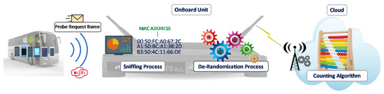
Figure 1.
iABACUS.
Every time a Wi-Fi device has to deliver a message, it needs to know which AP to access. This information is provided to the devices by the concept of association, which is a necessary, but not sufficient, operation to support the connectivity of the devices. Indeed, before a device is allowed to send a data message via an AP, it must first become associated with the AP. To this, the device sends Probe Request frames, i.e., messages broadcast periodically from any active Wi-Fi interface to detect nearby APs.
The core of the proposed system is a Wi-Fi sniffer that collects and analyzes the Probe Request frames; these frames include information that can be associated univocally to the device that sent them, thus enabling its identification and counting. Indeed, as shown in Figure 2 (Note that the purpose of Figure 2 is not to describe the fields of a Probe Request frame, but just to show its structure. The interested reader is referred to [44] for further details about the standard.), one of the fields of the Probe Request frame is the MAC address of the source (SA), which is univocally assigned by the manufacturer to the Wi-Fi interface. Therefore, common Wi-Fi-based APCSs are able to find the number of different devices located close to the sniffer by counting the number of different MAC addresses identified in the received Probe Request frames.
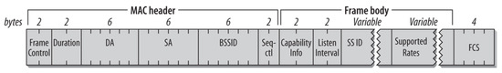
Figure 2.
Wi-Fi Probe Request frame [44].
Nevertheless, current Wi-Fi-based APCS based on MAC identification can effectively work only for obsolete operating systems (earlier than Android 5.0, iOS 7 and Windows Phone 8). In fact, with the aim to protect their users’ privacy against device tracking, the main mobile operating system providers have introduced software randomization of MAC addresses [16]: the MAC address included in Probe Request frames is not the real MAC address associated to the Wi-Fi interface anymore, but it rather is randomly generated and it periodically changes.
The characteristic that differentiates random MAC addresses from non-random ones is the fact that the first 6 octets of non-random MAC addresses are characterized by the Organizationally Unique Identifier (OUI), which is assigned by the Institute of Electrical and Electronics Engineers (IEEE) and identifies the manufacturers of existing network cards. Accordingly, the first 6 octets of the MAC address included in a Probe Request frame are compared with the list of all the OUIs that are associated to existing manufacturers of network cards. As depicted in Figure 1, if the MAC address is identified as a random MAC address, i.e., its first 6 octets do not correspond to any existing OUI, the de-randomization algorithm is run right after the sniffing process, before the counting algorithm. Otherwise, no de-randomization is needed, and the Probe Request can be passed directly to the counting algorithm. The main goal of the counting algorithm is to understand which of the Probe Requests received come from devices that are actually on the bus or are received due to cars or people moving near it.
In the following, the de-randomization process and the counting algorithm will be described in details.
3.1. De-Randomization Algorithm
The randomization of the MAC address introduced by operating system providers has allowed to hide the real MAC address of the network cards in the Probe Request frames of the device from which they are sent. In the Probe Request frames the real MAC addresses are replaced by random MAC addresses that are changed several times over a limited period of time. The change does not take place at regular intervals or according to predefined timing, but depending on the use of the device. Therefore the MAC address contained in the Probe Request frames is no longer sufficient to count the devices as it previously happened.
In this Section we introduce the de-randomization algorithm, which has the purpose to understand which MAC addresses are more likely to be brought back to the same device. Indeed, some parameters included in Probe Request frames can be exploited to estimate with sufficient reliability which frames containing different random MAC addresses may have been sent by the same device.
In particular, some fields of Probe Request frames remain constant even with randomized MAC addresses, as highlighted by the red square in Figure 3, also called tagged parameters [44].
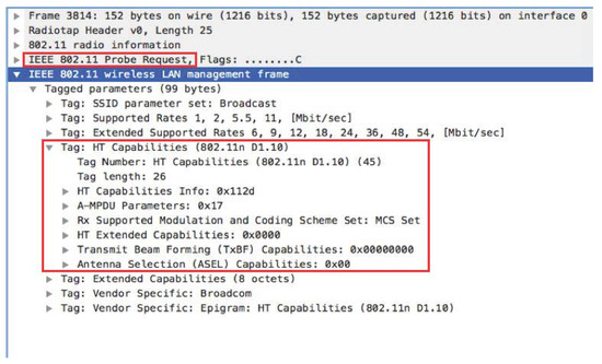
Figure 3.
Tag Section Probe Request Frame.
This information is the same in all the Probe Request frames sent by the same device, even if the MAC address is randomized. However, this information identifies a particular family of devices but not the single device. In order for two frames containing different random MAC addresses to be traceable to the same device, the fact that these information are the same must therefore be considered as the first condition, necessary but not sufficient.
The de-randomization algorithm therefore needs to exploit other parameters, whose changes provide important information. Let us consider two MAC addresses received from the sniffer, namely and with received before . Accordingly, in order for the two MAC addresses to be traced back to the same source device, the instant of time when was received, namely its timestamp, has to be lower than ’s timestamp. Therefore, calling and the tagged parameters of respectively and , the last timestamp associated to and the first timestamp associated to (both expressed in seconds), the de-randomization algorithm starts if, and only if, both the following conditions are met:
where the first condition of Equation (1) selects only devices that have the same transmitting characteristics, i.e., same tagged parameters, whilst the second condition of Equation (1) ensures that the last frame with was sent before the first frame with .
As stated above, the de-randomization algorithm assesses the probability that two random MAC addresses correspond to the same device. To compute this probability, we define a score for each couple of random MAC addresses identified. The score is calculated using the timestamp and another relevant parameter included in the Probe Request: the frame sequence number. The sequence number is a 12-bit code that progressively increases with each frame and is contained in the Sequence control (Seq-ctl in Figure 2). Its value varies from 0 to 4095 and once this maximum value is reached the numbering starts again from 0. Successive frames have increasing sequence numbers, even if the random MAC address changes.
The score is in inverse proportion to the difference in time and the difference in the sequence numbers between received frames with different MAC addresses. The difference in time is expressed as as:
which expresses the continuity in the arrival of the frames, even for randomized addresses, and then guarantees that not too much time has passed since the change of address. The difference in the sequence numbers has a similar goal, i.e., to check the continuity in the received frames even if the MAC address is changed due to the randomization process. However, we need to take into account that the sequence number assumes values between 0 and 4095. Defining the sequence number of the last frame corresponding to and the sequence number of the first frame corresponding to , the resulting formula is the following:
The score used in the algorithm is then defined as:
The score assumes values higher than 0 only if Equation (1) holds, i.e., if j and i have the same tagged parameters and they are received one after the other. For values higher than 0, the greater the value, the greater the probability that two MAC addresses are attributable to the same source device.
Once the score has been calculated for all the couples of random MAC addresses identified, the algorithm has the task of creating lists of MAC addresses traceable to the same source device. The process to create lists, depicted in the flowchart of Figure 4, is now explained. Whenever a frame with a new random MAC address is received, the score is computed between and all the other random MAC addresses that are already in a list. If no lists have been created yet, no scores will be computed; if all the scores are equal to 0, certainly belongs to a new device. In both these case, a new list with as the only element is created. Otherwise, the address with the highest score with , i.e., with the highest probability to belong to the same device, is identified. Considering the list where is located, if is the last element of the list, is appended to the list. If there is another MAC address that follows in list , the has to be compared to : if the first is lower than the latter, it means that it is more likely that and belong to the same device, with respect to and . Therefore, the process to find the right list for starts again ignoring m. If, on the other hand, is higher than , the probability that and belong to the same device is higher than the probability that and do. Accordingly, is put in right after . Furthermore, the following MAC addresses in list are not sure to belong to the same device anymore. Hence, the process is repeated again for and all its following MAC addresses in .
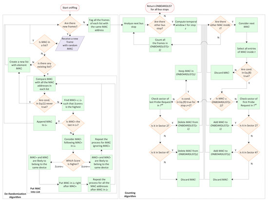
Figure 4.
Flow chart of the system.
The procedure therefore assumes a recursive form. At the end, all the lists are those with greater probability that the MAC addresses present therein are traceable to the same device. Accordingly, all the frames belonging to the same list are tagged with the same MAC address.
3.2. Passenger Counting Algorithm
Once the de-randomization process is solved, we need to analyze the resulting data, which represent the univocal MAC addresses of the sensed devices, in order to count the number of people on the bus.
With respect to a static situation, e.g., when counting people in a room, there are several issues that needs to be considered in order to accurately count only the people on the bus.
- the distance between two consecutive bus stops can be highly variable, from hundredth of meters to one-two kilometers;
- the Probe Requests are not sent regularly;
- the time the bus spends at each stop is variable and there may be stops where the bus does not stop;
- the sniffer can sense devices that are not on the bus, but are walking in the footpath, waiting at the bus stop or in the car near to the bus;
Let us consider the scenario depicted in Figure 5; our goal is to count the number of people on the bus and to know how many people board and alight from the bus during the last stop. To this, we define the set of bus stops , so that for each stop z, we can define the time of arrival at the bus stop and the time of departure from it ; then, we call time spent, the time interval the bus spends at each stop, which can be identified as follows:
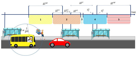
Figure 5.
Counting problem and parameters.
We can also identify the running time as the time the bus needs in order to run from one stop to the next one as follows:
In order to overcome the issues mentioned earlier, we need to filter all the entries in our database. To address the variability in the reception frequency of the Probe Requests, for every stop z we need to examine a temporal window so to consider for the counting algorithm only the Probe Requests received with an instant of time included in the interval:
where is a fixed parameter, called watch time.
After the temporal filtering, we need to understand if the remaining Probe Requests are transmitted by devices on the bus. To this, we applied a series of checks to all the entries in the filtered window. A first check is carried out to count the number of frames for each MAC address, namely , in order to identify devices encountered only for brief moments during the movement of the bus, such as the smartphone of a pedestrian or of a driver: if the number of frames captured is below a given threshold x, then the requests of these devices have been probably captured only a few times by the sniffer and then should be discarded.
Another check is implemented to evaluate the received power from the Probe Requests: received power is inversely proportional to the distance at which the transmitting device is located with respect to the sniffer, so it is possible to discard all the Probe Requests from devices which are too far and then are likely to be outside the bus, such as the case of a car that is moving in front of the bus as shown in Figure 5. In particular, we consider that the average power of the Probe Requests from received by the sniffer must be higher than a certain threshold , i.e., that ; doing so, it is possible to discard even the cases of a car in a traffic jam which constantly moves away (lower power) and gets together again with the bus (higher power).
Finally, due to how Probe Requests are sent, i.e., through a train of near-time requests, we decided to consider another parameter, namely the permanence of a device on the bus , calculated as the difference between the last and the first frame received in the temporal window, namely and , to assess if the requests belong to different trains of requests.
Summarizing, the entries of the generic address inside a temporal window, as defined by Equation (7), are considered for the counting algorithm if they satisfy the following conditions:
The number of unique MAC addresses left after the filtering steps gives a rough estimate of the number of devices on the bus. However, it is still important to assess at which stop the device boards and alights. This information is really useful to construct origin–destination matrices, but also to assess that the first or the last occurrence of a MAC address is not too far from any stops, thus indicating another vehicle travelling close to the bus with a similar speed, rather than a passenger boarding or alighting from the bus in motion.
To this, we consider that a device boarded or alighted from the bus only if the first or last Probe Request was received in a time frame of the bus stop, respectively. This is necessary because it is not possible to know in advance when the Probe Requests will be transmitted, so we must guarantee a guard time, both before arriving at the bus stop, , and after leaving it, , for those unlucky cases in which the first or the last Probe Request is sent just before reaching the bus stop or shortly after leaving it.
For every bus stop with a , there will be a time frame of available to receive the first or last Probe Request from a device. In general, the guard time can be considered constant for all the stops both before and after each stop, so we can indicate it as ; however, if the running time between two stops is too small, i.e., less than , then the guard time must be modified accordingly as .
We finally need to understand, for each temporal window and for each device, if the device was actually on board and if it boarded or alighted during the considered timeframe. As shown in Figure 5, when analyzing a single timeframe, we can individuate different sectors:
- Sector 1, between the start of the temporal window and the start of the guard time for stop .
- Sector 2, which analyzes the stop , considering both the guard times, before and after the stop, and the time spent.
- Sector 3 examines the time between two stops.
- Sector 4, which takes into account the event for stop z.
- Sector 5, between the end of the guard time for stop z and the temporal window.
For each device, the counting algorithm first checks if the device was already considered on board. If it is the first time the sniffer has received requests from the device, the algorithm has to understand at which stop the device boarded: as we said earlier, a device can only board if the first Probe Request, , has been received when the bus is near a bus stop. The device will be counted as boarding at stop if the first Probe Request is received in Sector 2 or at stop z if it is received in Sector 4. In all the other cases, i.e., when the Probe Request is received inside Sector 1, 3 and 5, all the entries for the device are considered as spurious and then discarded.
An on board device is considered as such for the whole temporal window; in this situation the condition on the number of frames for the next temporal window, described in Equation (7), is updates as follows:
to take into account that the device is already on board. However, if the device does not pass the filtering step in the next temporal window, i.e., for stop , then the algorithm goes back to the previous temporal window to check what happened by analyzing the last Probe Request received, . Again, a device will be counted as alighting from the bus at stop or z only if the last Probe Request is received in Sector 2 or 4 respectively, otherwise all the entries for the device are discarded.
Noteworthy, every time the bus reaches a stop z, the algorithm is able to count the number of passengers related to the previous stop, by checking the next temporal window.
Figure 4 illustrates all the steps of the overall process. It starts with the sniffing of the Probe Requests and ends when all the bus stops have been analyzed to count the passengers.
4. Experiments
In this Section, the performance of iABACUS is evaluated. The setup of the experiments consists of a Wireshark sniffer, set in Monitor Mode, with a filter that picks up only Probe Request frames with broadcast destination address, i.e., ff:ff:ff:ff:ff:ff. The captured frames are sent to a MySQL database where they are collected and stored. To this, a connection is established by a Lua script, which forwards the captured frames to the database. The database is then queried thanks to a PHP application.
In the following, the experiments’ results based on this setup will be shown. The first experiments, shown in Section 4.1, were made to test the de-randomization algorithm in a static scenario. Later, Section 4.2 presents the tests made to count passengers in a dynamic scenario.
4.1. Accuracy Evaluation for the De-Randomization Algorithm
The first tests were carried out in a static scenario, specifically to assess the accuracy of the de-randomization algorithm. Test results rely on the number of devices identified after the de-randomization process, i.e., the number of lists that are produced as output of the De-Randomization Algorithm described in Section 3.1
The experiments were run in a university room in a time window of 15 minutes. The following information was collected from the device owners inside the room: number of devices with active Wi-Fi interface; real MAC addresses of devices; brand, operating system type and version of devices.
The first parameter that was considered in the experiments is the transmission frequency. Indeed, according to the standard, the typical transmission frequency bands for Wi-Fi are and 5 GHz. Nevertheless, while all the detected devices transmitted at GHz, this was not always verified at 5 GHz. Furthermore, the GHz Probe Request frames are the most complete and information-rich. Therefore, the 2.4 GHz was chosen as receiving frequency for the Wireshark sniffer. The possibility of gathering information on both frequencies was also assessed. However, since a sniffer can capture data only at one frequency at a time, this would require two sniffers placed in the same point. Furthermore, the process of combining the capture of the two sniffers and analyzing many more frames would significantly increase the computational load of the system, while not providing significant further information. For these reasons, the reception frequency was set to GHz.
In order to set the most appropriate power threshold , which limits the considered devices to those that are inside the room, the average power of all the Probe Request frames received, shown in Figure 6, was evaluated. As expected, the highest average power was measured for the devices that were closer to the sniffer. In addition, it can be noted that there is a distinct division between received power values higher than dBm and lower than dBm. Along with the distance, this latter higher attenuation can be ascribed to the presence of walls. Accordingly, the power threshold was set to dBm. The parameters that were used for this test are summarized in Table 3.
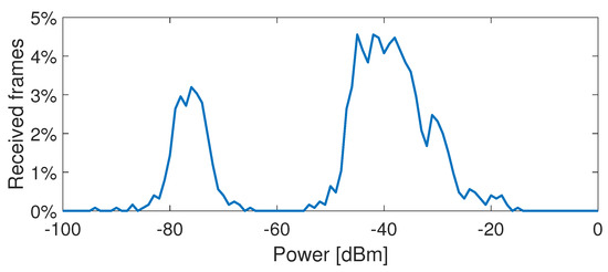
Figure 6.
Percentage of received Probe Request frames with respect to their receiving power.
Table 3.
Parameters of the experiments for the evaluation of the accuracy performance of the de-randomization algorithm.
The final results of iABACUS tested in this static case are shown in Table 4, where the number of MAC addresses counted by the proposed algorithm is compared with the number of MAC addresses counted by common Wi-Fi-based APCSs, i.e., systems that do not take into account the randomization of the MAC address and simply count the number of unique MAC addresses identified. As can be seen from the data in the table, iABACUS ensures that a much more accurate result is obtained, compared to common Wi-Fi-based APCS that does not take into account the randomization of MAC addresses. In particular, the system returned the exact number of devices present in the room (i.e., 21), while a traditional procedure would have recorded a significantly higher number of devices (i.e., 37). Since common Wi-Fi-based APCSs can only understand if a MAC address is random, and not if two different random MAC addresses can be associated to the same device, they associate a device to each different random MAC address received. Therefore, their error on the number of devices that implement the MAC address randomization is tied by the observation time window, that in this case was equal to 15 minutes: the longer the time window, the higher the number of times a device changes its MAC address and then the higher the number of devices counted.
Table 4.
Results for the accuracy evaluation of the de-randomization algorithm.
4.2. Passenger Counting Experiments
To evaluate the feasibility and performance of the proposed counting algorithm, a real dynamic environment has been reproduced. The main characteristic of this dynamic scenario is the possibility for people to move in and out of the sniffer caption’s range due to the movement of the sniffer itself. This is the case of a sniffer inside a bus where people board and alight during bus stops.
The experiments were performed in the city of Cagliari, Italy. To limit their randomness, we made use of a car to simulate an existing bus path both in the bus stops’ positions and for their time spent. The car’s path is shown in Figure 7, which also highlights the 13 stops considered. The number of Wi-Fi devices involved is limited to 8, with three of them implementing the randomization of the MAC address. The events of people boarding and alighting from the bus were simulated by switching on and off the Wi-Fi interface of the devices respectively. The plan of the experiments is shown in Table 5, which represents for each device, labelled from device A to device H, the origin’ and destination’ stop; Table 5 also shows the results of the three tests performed, that will be discussed below, highlighting in pale blue color the cells where something wrong happened. All the experiments were carried out before or during the lunch break, in moderate traffic conditions. The path is around 2.4 km long and has three traffic lights: the car needed around 15 min to travel it, which is an average time also for a passenger travelling on the bus.
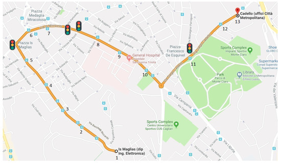
Figure 7.
Path of the vehicle for the experiments.
Table 5.
Origin and Destination matrix.
For the sniffer, the same setup described in Section 4 has been implemented on a Raspberry Pi 2 with Raspbian Stretch as Operating System to improve the portability of the solution. A USB Wi-Fi dongle is used as antenna to enable the Raspberry to collect the Probe Requests. The car’s path has been monitored with a GPS module (GPS GY-NEO-6M v2), sending its position (latitude and longitude) to the Raspberry every 5 s. The GPS information is essential to obtain the time of arrival and the time of departure from each bus stop, as well as the running time , which are key parameters for our counting algorithm. Moreover, the GPS enables the spatial mapping with the Probe Requests received by the Raspberry by comparing their timestamp.
Table 6 summarizes the value of the parameters considered during the performed tests. We have chosen reasonable values for the parameters in the first test; we then analyze the results of each test, comparing them with the planned experiment in order to tune them in the subsequent tests and correct the errors of the algorithm.
Table 6.
Setting Parameters.
The results of the first test show that devices A and H are missing, device D boards at stop 4 instead of stop 2 while device C alights at stop 8 instead of stop 9; moreover, we individuated a new device, labelled as X, that was not planned in the experiment, boarding at stop 3 and alighting at stop 5. We then analyzed step by step what happened during the trip:
- during the temporal filtering less than 5 occurrences of the requests for devices A and H were found, so since they were on board for only one stop, they were discarded from the algorithm; during our experiments, devices usually send a train of probe requests, i.e., a group of requests, every 40 s, but devices in energy-saving mode can send these requests with a lower frequency. By studying the capture from the sniffer, we notices that the frequency of the probe requests from devices A and H was really low, around 2–3 min, meaning that the devices were in energy saving mode.
- We have entries of device D from the temporal window of bus stop 2, unfortunately none of those entries were in the right Sector in order to count the device as on board, until the car arrived at the bus stop 4.
- Regarding device C, when analyzing bus stop 9, we found too few entries (only 3), so we checked the previous bus stop, i.e., bus stop 8, and found that the device last probe request was in Sector 4, so the algorithm signed the device as alighting at stop 8.
- Finally, between stop 3 and stop 5 we got stuck in a little traffic jam, so we needed a lot of time to travel this road section and our algorithm was able to accumulate a lot of entries from another device, maybe a smartphone from a car travelling behind or in front of us, that was then counted as a passenger on board.
For the second test, we increased the temporal window from 2 to 4 min and reduced the required number of frame from 5 to 3, in order to enable even the devices in energy save mode to be counted correctly; moreover, we also increased the guard time , so that it was more likely to find a device in the right bus stop, both boarding or alighting. We also decide to set a more conservative threshold for the received power, to avoid counting devices from outside the car.
From the analysis of the second test, we found only one error: device C alights at bus stop 3 but boards again at stop 5 to finish its trip correctly at stop 9. By checking the requests sent by the device, we noticed that they were fairly regular (about one train of requests every 42 s), but for some reason, around stop 3 and 5, the sniffer has missed some of them, resulting in the strange behaviour detected. However, we noticed that all the previous error were corrected, so we decided only to further reduce the number of frames required for a MAC address to be considered by the counting algorithm.
From the third test, we noticed that the problem regarding device C was solved and that no external devices were counted, even with a number of frames required equals to 1: this is due to the ability of the algorithm to filter out most of the probe requests thanks to the power threshold. However, we detected that device D was counted again as boarding at a different bus stop, as it happened during the first test, but not in the second one; this happens since stop 2 and 3 are really close, so that there is no Sector 3 among them and the two guard times from stop 2 and stop 3 overlap. Device D is then counted as boarding based on the first probe request received: in the unlucky case, that the probe request is delayed to stop 3, this will result as an error, that can not be avoided.
From these tests, we can infer simple rules to set the algorithm’s parameters. The main goal is not to discard any device on the bus, even if they are in energy saving mode: to this, the temporal window should be quite large to be sure to detect at least one Probe Request, while the number of frames lose significance. Devices outside of the bus need then to be discarded through the use of the other parameters, such as the power threshold. However, these rules can only provide a first hint on the setting, since the algorithm needs to be adjusted based on the particular route and city under consideration.
5. Conclusions and Future Works
This paper proposed iABACUS, a novel automatic passenger counting system based on IoT for public transportation, which infers the number of people on-board based on Wi-Fi probe requests received by a sniffer installed on the bus. Due to the randomization of the MAC addresses, introduced with the latest mobile operating systems, current APCSs based on Wi-Fi are now obsolete. For this reason, iABACUS includes a de-randomization algorithm in order to understand which MAC addresses are more likely to be brought back to the same device; tests of the proposed algorithm on a total of 21 devices show that it is able to successfully recognize all the randomized MAC address. Moreover, our tests also highlight that the randomization of the MAC addresses is a serious problem, since even the presence of only three devices can lead to a count six times higher in a 15 min time interval.
We then investigated the counting algorithm by means of real experiments, simulating the bus behaviour with a car and considering eight passengers, boarding and alighting in different bus stops. Experiments are performed in stress conditions, in order to underline any problem with the algorithm. The results are quite good, as the counting algorithm, when set correctly, is able to count all the passengers; however, due to the low frequency with which devices send their probe requests, there may be random errors concerning the correct boarding and alighting from the bus of passengers.
As future works, we plan to consider how real use-case conditions, such as attenuation of the received Wi-Fi signal due to bus size or absorption by passenger bodies (especially for crowded buses), interference, and non-line-of-sight, affect iABACUS’s performance. We will study how many sniffers are required and their optimal position, in order to discern correctly the power of all the devices on-board w.r.t. the ones outside: using more than one sniffer, maybe set to accumulate requests in a different frequency channel, and aggregating their results, could prove to be a better approach. Finally, we plan to study the random error related to the proximity of two bus stops in order to find a relation with the probability of its occurrence. Moreover, we plan to study the systematic error due to the non-connected users in our system; to this, we aim to compare the results of the proposed algorithm with the computed number of passengers estimated by the local bus transport in the city of Cagliari and propose an adjusting factor to be applied to our system. There are certainly differences among cities in the number of non-connected users, so we expect that a similar methodology should be carried out in every city.
Author Contributions
Conceptualization, all; methodology, all; software, F.P. and L.P.; validation, M.N., F.P., L.P. and V.P.; formal analysis, all; investigation, M.N., F.P., L.P. and V.P.; resources, M.N., V.P. and B.B.; data curation, M.N., F.P., L.P., V.P.; writing—original draft preparation, all; writing—review and editing, M.N., V.P. and B.B.; visualization, all; supervision, M.N., V.P. and B.B. All authors have read and agreed to the published version of the manuscript.
Funding
This work was partially supported by the Italian Ministry of University and Research (MIUR), within the Smart Cities framework (Project CagliariPort2020, ID: SCN_00281 and Project Cagliari2020, ID: PON04a2_00381), and by the Italian Ministry of Economic Development (MiSE, Project INSIEME, HORIZON 2020, PON 2014/2020 POS. 395).
Conflicts of Interest
The authors declare no conflict of interest.
References
- Gong, H.; Chen, C.; Bialostozky, E.; Lawson, C.T. A GPS/GIS method for travel mode detection in New York City. Comput. Environ. Urban Syst. 2012, 36, 131–139. [Google Scholar] [CrossRef]
- Kaiser, M.S.; Lwin, K.T.; Mahmud, M.; Hajializadeh, D.; Chaipimonplin, T.; Sarhan, A.; Hossain, M.A. Advances in Crowd Analysis for Urban Applications Through Urban Event Detection. Proc. IEEE Trans. Intell. Transp. Syst. 2017, 19, 3092–3112. [Google Scholar] [CrossRef]
- Zhang, F.; Jin, B.; Wang, Z.; Liu, H.; Hu, J.; Zhang, L. On geocasting over urban bus-based networks by mining trajectories. IEEE Trans. Intell. Transp. Syst. 2016, 17, 1734–1747. [Google Scholar] [CrossRef]
- Zhang, J.; Shen, D.; Tu, L.; Zhang, F.; Xu, C.; Wang, Y.; Tian, C.; Li, X.; Huang, B.; Li, Z. A real-time passenger flow estimation and prediction method for urban bus transit systems. IEEE Trans. Intell. Transp. Syst. 2017, 18, 3168–3178. [Google Scholar] [CrossRef]
- Barabino, B.; Deiana, E.; Mozzoni, S. The quality of public transport service: The 13816 standard and a methodological approach to an Italian case. Ing. Ferrov. 2013, 68, 475–499. [Google Scholar]
- Pinna, I.; Dalla Chiara, B.; Deflorio, F. Automatic passenger counting and vehicle load monitoring. Ing. Ferrov. 2010, 65, 101–138. [Google Scholar]
- Barabino, B.; Di Francesco, M.; Mozzoni, S. An offline framework for handling automatic passenger counting raw data. IEEE Trans. Intell. Transp. Syst. 2014, 15, 2443–2456. [Google Scholar] [CrossRef]
- Chen, C.H.; Chang, Y.C.; Chen, T.Y.; Wang, D.J. People counting system for getting in/out of a bus based on video processing. In Proceedings of the Eighth International Conference on Intelligent Systems Design and Applications, 2008, ISDA’08, Kaohsiung, Taiwan, 26–28 November 2008; Volume 3, pp. 565–569. [Google Scholar]
- Gonzalez, M.C.; Hidalgo, C.A.; Barabasi, A.L. Understanding individual human mobility patterns. Nature 2008, 453, 779. [Google Scholar] [CrossRef]
- Sohn, K.; Kim, D. Dynamic origin–destination flow estimation using cellular communication system. IEEE Trans. Veh. Technol. 2008, 57, 2703–2713. [Google Scholar] [CrossRef]
- Wang, Y.; Chen, Y.J.; Yang, J.; Gruteser, M.; Martin, R.P.; Liu, H.; Liu, L.; Karatas, C. Determining driver phone use by exploiting smartphone integrated sensors. IEEE Trans. Mob. Comput. 2015, 15, 1965–1981. [Google Scholar] [CrossRef]
- Pompei, F. Geolocation for LPT: Use of geolocation technologies for performance improvement and test of Local Public Transport. In Proceedings of the 2017 IEEE International Conference on Environment and Electrical Engineering and 2017 IEEE Industrial and Commercial Power Systems Europe (EEEIC/I&CPS Europe), Milan, Italy, 1–5 July 2017; pp. 1–5. [Google Scholar]
- Santos, P.M.; Kholkine, L.; Cardote, A.; Aguiar, A. Context classifier for position-based user association control in vehicular hotspots. Comput. Commun. 2018, 121, 71–82. [Google Scholar] [CrossRef]
- Amsterdam Airport Schiphol. Royal Schiphol Group Privacy Statement. Available online: https://www.schiphol.nl/en/privacy-policy/. (accessed on 12 February 2019).
- Transport for London. Review of the TfL WiFi Pilot. Available online: http://content.tfl.gov.uk/review-tfl-wifi-pilot.pdf. (accessed on 12 February 2019).
- Myrvoll, T.A.; Håkegård, J.E.; Matsui, T.; Septier, F. Counting public transport passenger using WiFi signatures of mobile devices. In Proceedings of the 2017 IEEE 20th International Conference on Intelligent Transportation Systems (ITSC), Yokohama, Japan, 16–19 October 2017; pp. 1–6. [Google Scholar]
- Martin, J.; Mayberry, T.; Donahue, C.; Foppe, L.; Brown, L.; Riggins, C.; Rye, E.C.; Brown, D. A study of MAC address randomization in mobile devices and when it fails. Proc. Priv. Enhancing Technol. 2017, 2017, 365–383. [Google Scholar] [CrossRef]
- Smartphone Ownership Is Growing Rapidly around the World, but Not Always Equally. Available online: https://pewrsr.ch/2Ngqr32. (accessed on 10 October 2019).
- Nielsen, B.F.; Frølich, L.; Nielsen, O.A.; Filges, D. Estimating passenger numbers in trains using existing weighing capabilities. Transp. A Transp. Sci. 2014, 10, 502–517. [Google Scholar] [CrossRef]
- Attanucci, J.; Vozzolo, D. Assessment of Operational Effectiveness, Accuracy, and Costs of Automatic Passenger Counters; Number HS-037 821; Transportation Research Board: Washington, DC, USA, 1983. [Google Scholar]
- Furth, P.G.; Hemily, B.; Muller, T.; Strathman, J.G. Uses of archived AVL-APC data to improve transit performance and management: Review and potential. TCRP Web Doc. 2003, 23, 1–58. [Google Scholar]
- Boyle, D.K. Passenger Counting Systems; Number 77; Transportation Research Board: Washington, DC, USA, 2008. [Google Scholar]
- Kovács, R.; Nádai, L.; Horváth, G. Concept validation of an automatic passenger counting system for trams. In Proceedings of the 5th IEEE International Symposium on Applied Computational Intelligence and Informatics, SACI’09, Timisoara, Romania, 28–29 May 2009; pp. 211–216. [Google Scholar]
- Choi, J.W.; Quan, X.; Cho, S.H. Bi-directional passing people counting system based on IR-UWB radar sensors. IEEE Internet Things J. 2018, 5, 512–522. [Google Scholar] [CrossRef]
- Bartolini, F.; Cappellini, V.; Mecocci, A. Counting people getting in and out of a bus by real-time image-sequence processing. Image Vis. Comput. 1994, 12, 36–41. [Google Scholar] [CrossRef]
- Harasse, S.; Bonnaud, L.; Desvignes, M. Finding people in video streams by statistical modeling. In International Conference on Pattern Recognition and Image Analysis; Springer: Berlin, Germany, 2005; pp. 608–617. [Google Scholar]
- De Potter, P.; Kypraios, I.; Verstockt, S.; Poppe, C.; Van de Walle, R. Automatic Passengers Counting In Public Rail Transport Using Wavelets. Automatika 2012, 53, 321–334. [Google Scholar] [CrossRef]
- Xiang-Yang, S.; Hao-Wei, W. Study on Method of Multi-feature Reduction Based on Rough Set in Passenger Counting. In Proceedings of the 2016 IEEE International Conference on Industrial Informatics-Computing Technology, Intelligent Technology, Industrial Information Integration (ICIICII), Wuhan, China, 3–4 December 2016; pp. 307–310. [Google Scholar]
- Olivo, A.; Maternini, G.; Barabino, B. Empirical Study on the Accuracy and Precision of Automatic Passenger Counting in European Bus Services. Open Transp. J. 2019, 13, 250–260. [Google Scholar] [CrossRef]
- Demissie, M.G.; Phithakkitnukoon, S.; Sukhvibul, T.; Antunes, F.; Gomes, R.; Bento, C. Inferring passenger travel demand to improve urban mobility in developing countries using cell phone data: A case study of Senegal. IEEE Trans. Intell. Transp. Syst. 2016, 17, 2466–2478. [Google Scholar] [CrossRef]
- Gao, R.; Zhao, M.; Ye, T.; Ye, F.; Wang, Y.; Luo, G. Smartphone-based real time vehicle tracking in indoor parking structures. IEEE Trans. Mob. Comput. 2017, 16, 2023–2036. [Google Scholar] [CrossRef]
- Carrel, A.; Lau, P.S.; Mishalani, R.G.; Sengupta, R.; Walker, J.L. Quantifying transit travel experiences from the users’ perspective with high-resolution smartphone and vehicle location data: Methodologies, validation, and example analyses. Transp. Res. Part C Emerg. Technol. 2015, 58, 224–239. [Google Scholar] [CrossRef]
- Chaudhary, M.; Bansal, A.; Bansal, D.; Raman, B.; Ramakrishnan, K.; Aggarwal, N. Finding occupancy in buses using crowdsourced data from smartphones. In Proceedings of the 17th International Conference on Distributed Computing and Networking, Singapore, 4–7 January 2016; p. 35. [Google Scholar]
- Lu, Y.; Misra, A.; Wu, H. Smartphone sensing meets transport data: A collaborative framework for transportation service analytics. IEEE Trans. Mob. Comput. 2017, 17, 945–960. [Google Scholar] [CrossRef]
- Lee, U.; Magistretti, E.; Gerla, M.; Bellavista, P.; Corradi, A. Dissemination and harvesting of urban data using vehicular sensing platforms. IEEE Trans. Veh. Technol. 2009, 58, 882–901. [Google Scholar]
- Corsar, D.; Cottrill, C.; Beecroft, M.; Nelson, J.D.; Papangelis, K.; Edwards, P.; Velaga, N.; Sripada, S. Build an app and they will come? Lessons learnt from trialling the GetThereBus app in rural communities. IET Intell. Transp. Syst. 2017, 12, 194–201. [Google Scholar] [CrossRef]
- Susilo, Y.O.; Liotopoulos, F.K. Measuring Door-to-Door Journey Travel Satisfaction with a Mobile Phone App. In Quality of Life and Daily Travel; Springer: Berlin, Germany, 2018; pp. 119–138. [Google Scholar]
- Liu, H.; Yang, J.; Sidhom, S.; Wang, Y.; Chen, Y.; Ye, F. Accurate WiFi based localization for smartphones using peer assistance. IEEE Trans. Mob. Comput. 2013, 13, 2199–2214. [Google Scholar] [CrossRef]
- Casetti, C.E.; Chiasserini, C.F.; Duan, Y.; Giaccone, P.; Manriquez, A.P. Data connectivity and smart group formation in Wi-Fi Direct multi-group networks. IEEE Trans. Netw. Serv. Manag. 2017, 15, 245–259. [Google Scholar] [CrossRef]
- Kholkine, L.; Santos, P.M.; Cardote, A.; Aguiar, A. Detecting relative position of user devices and mobile access points. In Proceedings of the 2016 IEEE Vehicular Networking Conference (VNC), Columbus, OH, USA, 8–10 December 2016; pp. 1–8. [Google Scholar]
- Santos, P.M.; Rodrigues, J.G.; Cruz, S.B.; Lourenço, T.; d’Orey, P.M.; Luis, Y.; Rocha, C.; Sousa, S.; Crisóstomo, S.; Queirós, C.; et al. PortoLivingLab: An IoT-Based Sensing Platform for Smart Cities. IEEE Internet Things J. 2018, 5, 523–532. [Google Scholar] [CrossRef]
- Tu, L.; Wang, S.; Zhang, D.; Zhang, F.; He, T. ViFi-MobiScanner: Observe Human Mobility via Vehicular Internet Service. IEEE Trans. Intell. Transp. Syst. 2019, 1–13. [Google Scholar] [CrossRef]
- Kyritsis, D. The Identification of Road Modality and Occupancy Patterns by Wi-Fi Monitoring Sensors as a Way to Support the “Smart Cities” Concept: Application at the City Centre of Dordrecht. Master’s Thesis, TU Delft, Delft, The Netherlands, 2017. [Google Scholar]
- IEEE Computer Society LAN/MAN Standards Committee. IEEE Standard for Information Technology-Telecommunications and Information Exchange between Systems-Local and Metropolitan Area Networks-Specific Requirements Part 11: Wireless LAN Medium Access Control (MAC) and Physical Layer (PHY) Specifications; IEEE Std 802.11; IEEE: New York, NY, USA, 2007. [Google Scholar]


© 2020 by the authors. Licensee MDPI, Basel, Switzerland. This article is an open access article distributed under the terms and conditions of the Creative Commons Attribution (CC BY) license (http://creativecommons.org/licenses/by/4.0/).