Long-term Static and Operational Reserves Assessment Considering Operating and Market Agreements Representation to Multi-Area Systems

Abstract

This paper exploits different computational modelling to assess long-term static and operating reserves to multi-area systems. To deal with intermittent renewable generation and other types of technologies, this paper is proposing a flexible simulation model able to capture not only technological innovation of power system components and their electric and energetic behaviors, but also operational procedures and market agreements representations to yield planning insights about the performance of the multi-area systems. Results based on two modified test systems with a variate of generation technologies and interconnections are used to show the potential of the simulation model.

1. Introduction

The fast growing of the intermittent renewable generation, such as wind and solar photovoltaics, which have been watched across the countries and continental areas, has been demanding new planning and operating practices based on systemic studies [1]. In general, large systems, with extended interconnected areas, take systemic benefits into account as philosophy of operation, mainly based on generation and transmission systems technologies. The relationship among interconnected areas may be described through some systemic actions where supported areas are receiving constant assistance by areas of support, for instance, frequency response as ancillary service to ensure generation and load balance, among others [2].

Several large systems, since the foundations, have been growing and developing with huge investments over hydro and thermal electricity generation technologies and extended transmission lines. The hydrothermal optimization problem was always part of the planner’s and operator’s agenda, where synchronous machine directly connected to the grid are able to offer operational systemic benefits, such as inertial response, which is an essential ancillary service to ensure short-term supply and demand balancing throughout a power system. This service is assured only by synchronous generators, since they are able to provide system inertia throughout different control areas [3].

From an electricity generation perspective, the intermittent renewable generation offers not only social, economic, and environmental benefits, but also significant energetic gains to the grid, mainly due to the asynchronous characteristic of these technologies, which is in accordance with high levels of variability as encountered on wind and solar irradiance resources [4]. However, from a wind and solar energy point of view, either the wind turbines based on asynchronous machines or photovoltaic panels without rotative devices, the systemic benefits achieved are directed to energetic efficiency of the grid, and do not offer, for instance, inertial response as hydro and thermal generating units [5].

From a transmission system perspective, the High-Voltage Direct Current (HVDC) link, as an option to bring electricity from long distances, consists of a solution with less environmental impact and attrahent implementation costs. The maturity of power electronics apparatus [6] have inspired confidence in the planners and operators to use these technologies. On the one hand, this type of technology allows a decoupled system operation, avoiding transient events propagation across the system, which can be seen as a benefit to the system. On the other hand, a large number of HVDC transmission lines may be seen as a source of reduction of system services, where hydro and thermal generating units, when connected to these technologies, lack the ability to offering system services, such as inertial response.

Operating reserves can be categorized according to their time response to system changes [7]: regulating reserve, contingency reserve, and, more recently, renewables reserve [7]. Regulating reserve is usually provided by units with automatic generation control and with immediate time response. Contingency reserve, that can be categorized into spinning and non-spinning reserve, is used to a response to contingencies that may occur on systems, such as forced outages of generators or transmission lines. The contingency reserve time response is less than 10 min for the spinning reserve, and less than 1 h for the non-spinning reserve. In renewables reserves, the chosen units may have a slower response, since wind power variation occurs slower than the traditional contingencies, which may imply minor costs [7]. Applications of regulating reserves and contingency reserve are well known in the state of art and can be found in [8,9]. Applications of renewable reserves, in the short-term, can be found in [7,10]. The present study relies on the planning phase of the long-term operating reserve assessment, which aims to address short-term operational reserve aspects in assessing the adequacy of power systems.

Concerning these perspectives, the increased usage of intermittent renewable generation and HVDC links applications has constructed the current power system, where part of these systems may be viewed as synchronous and others parts as asynchronous. Regardless of these system characteristics, the effect of these application technologies on large systems requires a set of new criteria, methodologies, and models to establish a balance between synchronous and asynchronous system taken the security of supply into account. This paper approaches power system analysis from these new perspectives, where computational solutions are able to capture details of interconnected systems with high penetration of intermittent renewable generation, with different agreements of support between areas, considering long-term operational reserve evaluation, are necessary.

2. Theoretical Background

From a modern power system planning perspective, the simulation setup considered to evaluate the performance of a planned grid configuration should take not only the adequacy and security aspects into account [11], but also capture the behavior of new technologies throughout electric and energetic models, market rules, and operational procedures [12]. Simulation is being used to experiment with new scenarios so as to evaluate system behavior under new circumstances. By means of simulation studies, planners and operators may yield valuable insights of the system performance when, for instance, renewable variable generation and HVDC transmission lines are occupying a major portion of the technology portfolio of a modern power system.

2.1. Simulation Mechanism and Models Applied to Power System Planning

In general, the simulation mechanism may be viewed as the way to computationally represent a collection of related components to study a system. The simulation mechanism commonly used for planning purposes may be classified as dynamic, from a time perspective, where models represent a system that evolve over time allowing the representation of time dependent models [13]; stochastic, since random variables are used to represent the behaviors of the component; and discrete, since state variable change instantaneously at discrete points in time [14]. Regardless of the generating unit or transmission line technology, power system components may be computationally represented by the up and down operating cycle [13] using Markov models, which are discrete from the event perspective and continuous over the operation time [14]. Therefore, a combination of discrete-event simulation mechanism that evolves continuous over time has been used to capture electric and energetic behavior of components. First, the capacity and availability evaluation of system components is modeled, where power system planners may study generation capacity and transmission system availability throughout different long-term scenarios [8]. For several years, only this perspective of studies was used to assess long-term planning configurations [15]. However, a set of energetic concerns should also be considered to study long-term configurations in order to capture primary resources effects by each generating unit technology such as water inflow, wind intermittence, solar irradiance intermittence, and so on [8,9]. Generally, these models are built considering the historical time-series, allowing the characterization of hydro inflows over months, wind variability over minutes or hours, and solar irradiance over a different time step [16]. Usually, depending on the planning study, the scope of the assessment varies from nano-seconds to hours, and the simulation time step selected to model component behavior should be suitable enough in accordance with long-term configuration studied. In this context, a balance between simulation modeling and current technology should be considered, mainly because the uncertainty over 10 or 20 years ahead may be huge enough to decrease the credibility of the insights yielded.

Another major simulation modeling perspective are operational procedures and market rules representation, which may directly affect the system performance. The relationship between electric areas and/or countries requires a set of different rules based on unit commitment, dispatch actions, and interconnection availability [2,3], which may vary from market insights to security criterion over energetic and electric perspectives. For instance, it is possible to find several procedures for cross-border transmission capacity agreements around the world [12], mainly to determine the electric and energetic influence of neighboring areas, cross-border exchange limits, and technical and operational security criteria. These kinds of agreements establish not only operational procedure rules for security purposes, but also create market conditions. For instance, the definition of Net Transfer Capacity (NTC) and Available Transfer Capacity (ATC) in Europe and Australia are so important to market participants to anticipate and plan their cross-border business [2,3]. Nowadays, there are several proposals about operational procedures linked to market design, mainly to cover transient market power to avoid missing money problem [3]. The simulation model to approach this kind of problem can be classified as complex and time consuming from a computation point of view.

2.2. Statistical Analysis of Simulation Studies

An important part of the simulation study is the statistical output analysis established throughout the simulation model [14]. After defining the random vectors containing all the information about the power system, including component stochastic models and system operational and market procedures. The simulation process consists of the creation of repeated samples of the system states based upon a generation and transmission configuration that follows operational and market rules, in order to determine the follow expectation:

$$l=E\left[H\left(X\right)\right]=\int H\left(x\right) f\left(x\right)dx,$$

(1)

where $X$ is a random vector with probability density function (pdf) f. In other words, $X$ is a random vector, where power system components are experiencing up and down states under their stochastic parameters λ, μ (failure and repair rates), which are characterized by an exponential pdf here called f. $H\left(X\right)$, which is well known as a performance function that maps the whole set of sampled states. At this point, l (which is not possible to find analytically) may be statistically estimated as the sample mean:

$$\widehat{l}=N^{-1}{{\displaystyle \sum }}_{i=1}^{N}H\left(X_i\right),$$

(2)

where X₁,…,X_N is a random sample from f, and {Xi} are the independent replications of X considering f. The estimator is unbiased whether $E[\widehat{l}]=l$. Thus, by the law of large numbers, $\widehat{l}$ converges to l as Ν→∞ [14]. From a planning studies perspective, the following generic algorithm is usually coded to estimate the expectations:

• Select a system state X, i.e., define equipment availability, load levels, operating and market procedures, etc., in accordance with system representation;
• Calculate H(X) from the selected state, i.e., verify whether that specific configuration of generators and circuits is able to supply the specific load, without violating system limits and operating and market rules; if necessary, use remedial actions such as generation rescheduling, bus voltage corrections, bus load curtailments, etc.;
• Update the estimate of E[H(X)] based on the result of step (2), i.e., calculate reliability indices such as LOLP, EENS, etc. If the accuracy of the estimate is acceptable, stop; otherwise, return to step i.

The latter step of this generic algorithm denotes the needs of an acceptable estimate in order to stop the simulation process. From a statistic perspective, the accuracy of this particular $\widehat{l}$ should be accompanied by a confidence interval, where it is possible to verify how close $\widehat{l}$ is from l. Clearly, this distance represents a measure of dispersion in regard to the sampled mean, which usually supports the stop criterion used to control the length of a simulation process that is well known as relative error or coefficient of variation as following:

$$RE=\beta =\frac{\sqrt{Var\left(\widehat{l}\right)}}{E\left[\widehat{l}\right]}.$$

(3)

Additional details of this mathematical formulation can be found in [14].

3. The Evolution of Power System Representation

Simulation studies are used to assess different conditions concerning the system performance on power system analysis. Historically, the generation system reserve evaluation is decoupled into two-time frames, the planning and operating phases. The planning phase was concerned with the generation system to meet the long-term load forecast, whereas the operating phase was related to dealing with short-term load forecasts, where sufficient generation reserve should be scheduled to account for load uncertainties and sudden loss of generating units. A few years ago, the concept of operating reserve was extended to the planning phase [8,9], where the uncertainties linked to the intermittent renewable generation and a set of uncertainties of other types of technologies arose as new challenges to be faced on the planning of the future generation and transmission systems, so that they can deal with large levels of uncertainty (mainly wind and solar power and load forecasting errors) and fewer conventional generating units able to provide ancillary services to meet the load forecasted for the future. The framework used in [8] is partially presented in Figure 1, where static reserve evaluation remains with the same scope, but the operating reserve evaluation changes, assuming concerns linked to the long-term planning of electric system.

In this context, this paper proposes a set of generation and transmission planning representations to deal with long-term evaluations to planning studies. Figure 2 shows a set of planning system models to study long-term scenarios of generation and transmission systems, which involve single area and multi-area representations. Some of them are well-known in the technical literature, such as in Figure 2a,b,d; others characterize intermediate representations (Figure 2c,e), proposed by authors, to take some new insights into considerations during planning studies.

To deal with generation and transmission system assessment, a set of assumptions are necessary to evaluate the performance of the system components. For instance, a single bus representation shown in Figure 2a allows evaluating static and operating reserve, with different levels of details, from long-term perspective. In general, due to low computational costs, a sophisticated level of generating unit models can be applied to capture time dependent effects linked to intermittent renewable generation [13]. At this point, it is important to represent the primary resource behavior of each technology involved on the analysis. From a long-term perspective, single bus representation can be evolved to single bus multi-system, as shown in Figure 2c, where a set of different electric areas may be evaluated without transmission systems effects, but considering the same level of models used on single system evaluation. This type of representation allows to study different area agreements, where operating or market procedures can be tested considering high levels of intermittent renewable generation into electric areas. A natural evolution is to consider the transmission system effects among areas, as shown in Figure 2b, where interconnections may be represented, considering operating procedures and/or market rules among areas, as well as capacity constrains usually present in this type of evaluation. Moreover, it is possible to represent system services throughout different technologies of interconnections in order to differentiate HVDC from conventional systems.

Another set of simulation is characterized as composite analysis, where generation and transmission components are represented [17]. When the operator identifies a transmission circuit violation, such as operational limits, remedial actions are taken. From a simulation perspective, usually, power system analysis is represented by a linear DC model, where remedial actions, such as generation redispatch and/or load curtailment, are solved by a linear optimization formulation. One of the first grid representation, as shown in Figure 2d, consists of generating units, transmission circuits, and power transformers spatially represented over buses within an electric area. At this representation, it is possible to study different planning configurations of the grid, with an adequate level of the generating unit models [8], considering intermittent renewable generation and suitable models to capture transmission system constraints. In order to extend this representation as shown in Figure 2e, electric areas can be added to the evaluation, where composite assessment is merged with single bus evaluation to study agreements among areas considering a main system connected to different electric areas. The evolution of these representation allows planners to investigate the performance of interconnected system from a diverse number of perspectives.

3.1. Unit Commitment and Dispatch Representation

The unit commitment process aims to define the schedule of the generating units that will be dispatched for the next period, so they can be previously committed to be available at the time they are requested for dispatch. It follows an iterative process, based on a merit-order list, which may vary according to the scenario of availability of primary energy resources. In order to minimize the system operating cost, the adopted merit-order list relies on the individual operating cost of the generating units. It means that the lower the operating cost the higher the unit’s priority is to be dispatched. The unit commitment process ends when the following condition is satisfied:

$$G_{\mathrm{SYNC}}\ge G_L+R_P^{*}+R_S^{*}$$

(4)

where $G_{\mathrm{SYNC}}$ is the total capacity of synchronized generation, $G_L$ is the amount of generation mobilized to meet the estimated load of the period, and $R_P^{*}$ and $R_S^{*}$ are the primary and secondary reserve requirements, respectively, defined previously by the operator. These requirements are deterministic and may assume different values, according to the operation scenario. The tertiary reserve has no requirement as it corresponds to the non-synchronized portion, which, however, can be quickly mobilized, depending on the technology involved. The generation dispatch, in turn, aims to set the generators power dispatch at the operation time, based on the schedule of the unit commitment. The generation dispatch must be able to deal with the operation uncertainties, according to:

$$G_{REAL}=G_L+\Delta G+\Delta W+\Delta S+\Delta L,$$

(5)

where $G_{REAL}$ is the total generation performed at dispatch process during the system operation and ∆G, ∆W, ∆S, and ∆L are the uncertainties due to the generating units forced outages, wind forecast errors, solar forecast errors, and load forecast errors, respectively. Eventually, there may be transmission constraints on the transmission system, which prevent the optimal dispatch purely based on costs. All these effects lead to deviations from the generation schedule, resulting in changes of the individual dispatch of the generating units and, if necessary, the dispatch of out-of-merit-order generating units. Hence, the operating reserve amount are just used to face those needs unanticipated by the unit commitment process.

Moreover, a simple computational representation to address dynamic security aspects throughout adequacy studies is also proposed, based on [17]. Considering the concept of inertial load, which consists of a fixed set of generating units that due always be dispatched, independently of the hourly load variation, to supply a fixed fraction of the system load. In this work, a set of generating units is being dispatched during certain operating conditions, with the purposes to simulate a deterministic system stability criterion. Obviously, only by using dynamic assessment tools is it possible to determine the current degree of system security. However, this simple model allows to yield insights linked to security aspects observed by operators around the world.

3.2. Policy Representation of Multi-Area Systems

In order to properly determine the power exchange values between areas, it is necessary to represent the multi-area supporting policies adopted. Such policies result from the existing agreement between the operating agents of each system. Different policies lead to different exchange amounts and, consequently, different reliability indices for each area. To implement the power exchange policies in the simulation the use of linear programming models is necessary, as they allow the incorporation of support priority and restrictions between areas. In this work, three different multi-area policies were adopted:

• Assistance policy: each system performs the unit commitment on an individual basis, aiming at fulfilling the generation amounts necessary to meet the expected load of its own system, and its primary and secondary reserve requirements defined previously by the operator. This policy follows the no-load-loss sharing, that is, each system tries to meet its load within its own generation units and, if necessary, tries to cover the deficit through import action, if there is available capacity to export in neighboring systems. The export capacity of a given area corresponds to the amount of committed generation that was not used to meet its own load. Eventually, if more than one system needs support, a priority list is used to decide which area will have support priority.
• Market policy: the second multi-area policy allows for commercial exchanges between areas, making it possible for lower-cost generating units to be committed in neighboring areas. It means that the unit commitment process is carried out in a unified basis, so that generating units from any area can be committed to meet the load and reserve requirements of other areas. The power exchanges take place according to the spatial placement of the generating units among areas, defined after the joint commitment of all generating units. If there is a need of load-shedding due to generation deficit, the priority list of supported areas is used.
• Hybrid policy: the hybrid policy has characteristics of the two previous policies. Then, to cover the expected load needs of the systems, the unit commitment can be carried out looking for generating units in any of the interconnected areas, prioritizing those units with lowest operating cost. On the other hand, the unit commitment to meet reserve requirements is carried out on an individual basis. In other words, for load supply, systems can commit units in any area, and to meet their reserve requirements, systems should only use generating units in their own area. During the operation, if any area shows generation deficit, support can be sought in neighboring areas, limited to those units committed as tertiary reserve in the support areas. The power exchange between areas is, therefore, the result of the planned power exchanges to meet the expected loads and the eventual support to meet the uncertainties.

4. Case Studies and Numerical Experiments

After introducing the proposal of generation and transmission system representations, this section will evaluate two main perspectives of studies. First, a comparison about single bus and composite studies are posed from a mathematical perspective, where graph metrics are used to identify whether the transmission system has enough robustness to influence the simulation results significantly. Second, a planning exercise will be conducted in order to verify the significance of electrical models’ accuracy. Such computational representations should be deeply analyzed to take the energetic and capacity impacts into consideration during a simulation process. Moreover, the importance of the representation of the stochastic characteristics of electrical components should also be evaluated from a planning perspective, where the simulation process may be conducted, capturing the main phenomena linked to system failure effects, yielding insights to planners.

Bearing this concept in mind, this discussion will be carried out considering two well-known test systems and their variations to include new issues regarding hydro variation and renewable intermittence. The IEEE RTS 79 [18] system was designed by an IEEE task force to serve as a standardized test system for conducting tests and comparisons of power system reliability assessment methodologies. It is composed by 24 buses, 32 generating units, 33 transmission lines, and five power transformers. The total installed generation capacity is 3405 MW, comprising oil, coal, nuclear, and hydro units. The system total peak load is 2850 MW distributed among the system buses, and varying according to an 8736 steps of annual load profile, as provided in the original system. To complete 8760 h for a 365-day year, January 1st was replicated to December 31st. In order to highlight the effects of the fluctuations due renewable energy resources, two modifications were applied to the IEEE RTS 79 system. First, the fluctuation of the available hydro power is considered by means of an annual variation profile with a monthly basis, and the system is identified as IEEE RTS 79 H [19]. The second system modification considers the addition of 400 MW of new wind generating turbines concentrated on three wind farms, following an hourly based annual profile. This system is identified as IEEE RTS 79 HW [19].

The IEEE RTS 96 system [20] consists of three sets of the IEEE RTS 79 interconnected by transmission lines. It has 96 generating units, totaling 10,215 MW of capacity, and its transmission system consists of 104 lines and 16 power transformers. The total load is 8550 MW, distributed among the buses, and varying according to the same annual profile. The three systems are interconnected by five transmission lines. As the previous case, this system was also modified to consider the renewable resources fluctuation [9,21]. The first modification is the consideration of the available hydro fluctuation, renaming the system to IEEE RTS 96 H [9]. The second modification consists of substituting one coal unit of 350 MW by 1526 MW of wind power, increasing the total installed capacity to 11,391 MW. For both systems, short and long-term uncertainties of 2% and 1%, respectively, are considered over system load, following the uncertainty model presented in [8]. The wind uncertainty is based on persistence model [8].

4.1. Analysis of the Transmission System Representation

To deal with single system assessment, a single bus representation to planning purposes seems to be enough, when the planning study wishes verifying whether a generation portfolio is able to supply a system load from a long-term perspective. This is a very cheap computational evaluation with significant systems results to planners. Conversely, if the transmission system constraints need to be considered, depending on the level of the component modelling, the simulation study would become computationally expensive with other types of outputs. As previously mentioned, the use of one or another method of modelling can lead to different results, and these differences can be more or less significant according to the characteristics of the system. It is deemed that in cases where the transmission system is robust, i.e., causes little or no load-losses, both single-bus and complete network simulations tend to produce very close results. In such cases it is possible to give preference to the single-bus simulation without compromising the results once this simulation has the advantage of least computational effort, as it does not need the use of classic power system tools such as Power Flow Analysis and/or Optimal Power Flow techniques [17].

The purpose of the following analysis, prior to the beginning of the simulation, is to identify the characteristics of the system, which indicate the possibility of using single-bus analysis, without compromising the reliability indices. In other words, to identify system characteristics that indicate that the single-bus analysis may be sufficient, since the transmission network is robust enough and can be neglected. Therefore, two metrics were adopted to characterize the robustness of the transmission system:

• Average Degree or Valency of the network: this index is used in Graph Theory. The degree of a vertex V of a graph indicates the total number of edges that are incident to the vertex. In an electrical system, a vertex corresponds to a system bus and, therefore, the degree indicates the number of transmission lines and transformers that depart from each bus:

  $$\mathrm{deg}\left(V_i\right)=N{v}_i,$$

  (6)

  where $\mathrm{deg}\left(V_i\right)$ is the degree of the vertex $V_i$ and $N{v}_i$ is the number of edges that are incident to $V_i$. In the presented analysis, the average of the degree of all buses was considered to characterize the system:

  $$\mathrm{deg}\left(S\right)=Mean\left\{\mathrm{deg}\left(V\right)\right\},$$

  (7)

  where $\mathrm{deg}\left(S\right)$ is the degree of the system and $\mathrm{deg}\left(V\right)$ is the vector containing the degree values of all vertices of the system S. The degree of the system indicates how “meshed” the system is and, therefore, how much the failure of a network element tends to affect the capacity of the system to load supply.
• Capacity of Power Transfer: in addition to the degree of the network, it is also important to measure the capacity of the transmission lines that connect a given bus to meet its load. This capacity is limited by the individual power transfer capacities of each line. For a given bus, the used index in this work represents the relationship between the sum of the capacities of the lines and the value of the peak load connected to that same bus:

  $$cp\left(V_i\right)=\frac{{{\displaystyle \sum }}_{j=1}^{N{v}_i}{T}_j}{L_i},$$

  (8)

  where $cp\left(V_i\right)$ is the capacity index of $V_i$; $T_j$ is the transmission capacity of the $j_{th}$ line departing from $V_i$; and $L_i$ is the value of the peak load connected to $V_i$. To characterize the system, the average of the index values was considered for each bus:

  $$cp\left(S\right)=Mean\left\{cp\left(V\right)\right\},$$

  (9)

  where $cp\left(S\right)$ is the transmission capacity index of the system and $cp\left(V\right)$ corresponds to the vector containing the individual values of each bus. The presented analysis was based on the IEEE RTS 79 test system previously introduced, considering the operating reserve assessment to promote spatial distribution of the available generation, by means of Sequential Monte Carlo Simulation with a coefficient of variation β = 5%. Thus, it is proceeded as follows: first, the LOLE, EPNS, and LOLF reliability indices were obtained for the system in a single-bus evaluation, whose results were adopted as a reference; second, the transmission network metrics previously described were calculated and the same reliability indices were determined considering the transmission network; third, variations in the transmission network were promoted and, for each variation, the metrics were calculated and the values of the same set of reliability indices were obtained. The variations applied to the transmission network consists of changes in the capacity limits of the transmission lines and the addition/removal of lines connecting buses; finally, the obtained results were compared with the reference case (single bus evaluation). The

  Table 1. Transmission Network Metrics and Reliability Indices.

  Case	Description	Degree Index	Capacity Index	LOLE (h/year)	EPNS (MW)	LOLF (occ./year)
  Single-Bus	Reference case:Original system without the transmission network	-	-	10.13	0.14	3.24
  A	Original system with the transmission network	3.17	6.53	17.37	0.19	4.67
  B	2 times the number of lines	6.33	13.06	11.14	0.16	3.51
  C	3 times the number of lines	9.50	19.60	10.36	0.15	3.29
  D	4 times the number of lines	12.67	19.88	10.13	0.15	3.28
  E	4 times the number of lines + Lines capacity divided by 2	12.67	9.94	10.37	0.15	3.32
  F	4 times the number of lines + Lines capacity divided by 3	12.67	6.63	9.50	0.13	3.08
  G	4 times the number of lines + Lines capacity divided by 4	12.67	4.97	11.31	0.16	3.50
  H	3 times the number of lines + Lines capacity divided by 2	9.50	9.80	10.80	0.16	3.42
  I	3 times the number of lines +Lines capacity divided by 2	9.50	6.53	11.49	0.16	3.61
  J	3 times the number of lines +Lines capacity divided by 4	9.50	4.90	409.21	0.70	147.12
  K	2 times the number of lines +Lines capacity divided by 2	6.33	6.53	13.85	0.18	4.21
  L	2 times the number of lines +Lines capacity divided by 3	6.33	4.35	1,305.71	3.25	274.94
  M	2 times the number of lines +Lines capacity divided by 4	6.33	3.27	4,910.60	21.57	526.25
  N	Lines capacity divided by 2	3.17	13.06	12.49	0.15	3.54
  O	Lines capacity divided by 3	3.17	19.60	13.33	0.18	3.68
  P	Removal of duplicated lines	2.83	5.73	18.08	0.20	4.78

  presents the description and numeric results of each of the simulated cases.

Figure 3 shows the results of the simulated cases according to the LOLE and EPNS indices.

It can be seen that the cases closest to the reference (single-bus) are C, D, E, and possibly F. These are precisely those in which the system is most meshed, with an average degree of at least 9.5. In this case, a capacity index of approximately 7 already seems to be sufficient. However, if the system is not well meshed, as in the case of an N whose degree is 3.17, to obtain satisfactory results, the network capacity index must be at least 13. This type of evaluation could be significant to support planners’ decisions using single bus evaluation.

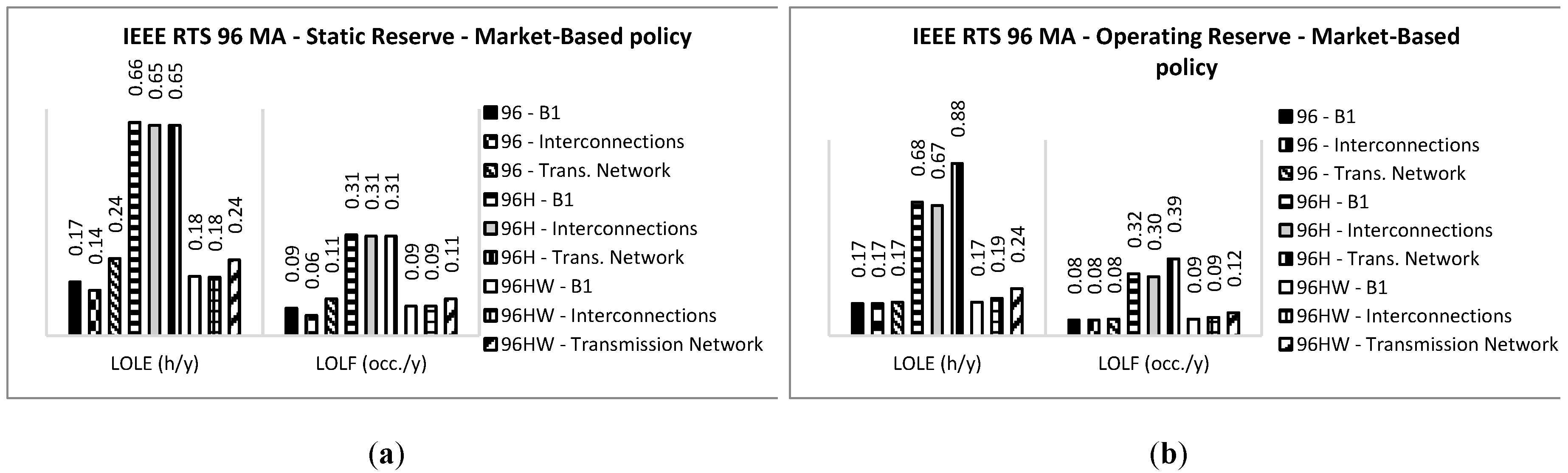
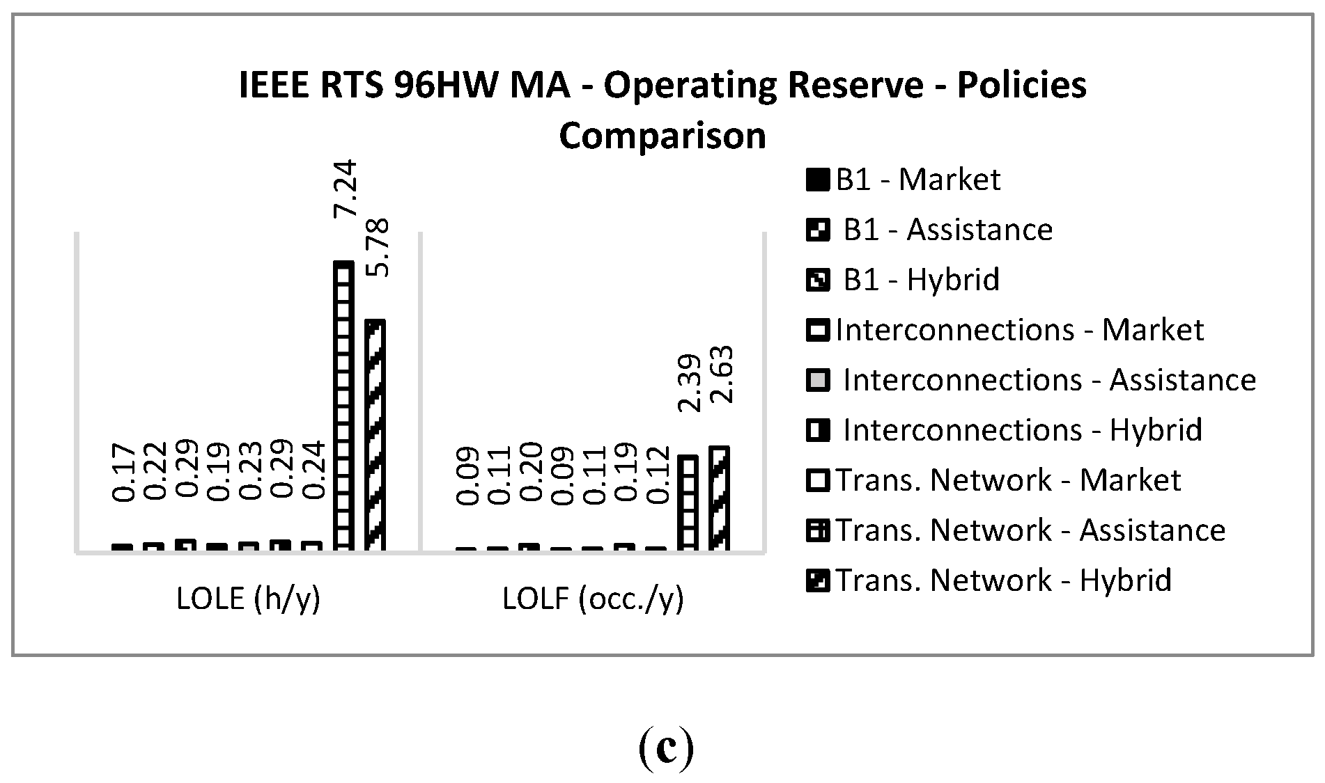
4.2. Risk Evaluation at Different System Representations

The first set of studies are based on the IEEE-RTS 79 test system (single area), which initially will be assessed by means of the static reserve and will discuss single bus and composite evaluations. The idea is to exploit three different scenarios: (a) the test system is simulated without any energetic model linked to the hydro subsystem and also without any intermittent renewable generation; (b) the test system is simulated considering an energetic model to the hydro subsystem, but remains without any intermittent renewable generation; (c) the test system is simulated considering an energetic model and consider the addition of wind power subsystem, bringing the intermittent effects of the renewable generation with them. Figure 4a shows these set of scenarios previously described. All these simulations are performed with a coefficient of convergence of 5%.

Bearing in mind the single bus evaluation described in scenario (a), where there is no energetic model linked to the hydro subsystem and no intermittent renewable generation, LOLE and LOLF indices perform a probability and a frequency of failures of 9.84 h/y and 3.21 occ./y, respectively. Both indices are inside the confidence interval proposed in this simulation process. One compares this single bus evaluation with the same scenario, but considering the composite evaluation, it is possible to see a slight increment of the result, where LOLE increase to 10.88 h/y and LOLF to 3.40 occ./y. In fact, this system has a robust transmission system, as it was discussed in Section 4.1. However, when an energetic model is considered, by means of scenario (b), the hydro availability is reduced causing a consequent escalation of the system risk, the LOLE index grows to 17.52 h/y and the LOLF index grows to 5.33 occ./y, respectively. Although the system risk has been increased, the behavior of the single bus and composite evaluations seems remained the same, with a slight difference between evaluations. At this point, it is mandatory to highlight the significance of energetic models for this type of planning study.

The simulation of the scenario (c) revels the importance of the wind power subsystem. On the one hand, the intermittent renewable generation brings a set of uncertainties with them, further complicating certain operational procedures. On the other hand, the additional distributed capacity alongside the system clearly mitigates the system risk; the LOLE index decreases to 6.80 h/y and the LOLF index decreases to 1.53 occ./y. Once again, the behavior of the indices, when single bus and composite evaluations are compared, seemingly remained the same, with a slightly difference between evaluations.

Taking these first set of studies into consideration, it is likely to identify a crescent difference between single bus and composite evaluations among each scenario. After comparing the scenarios, the difference between single bus and composite evaluations among each scenario increased in terms of LOLE and LOLF. Considering the LOLE index, the difference has increased from 9.56% to 11.25%, and to 23.77%, respectively; and in terms of the LOLF index, the difference has increased from 5.59% to 7.47%, and to 44.77%, respectively. In fact, less electricity production caused by the addition of energetic model and the spatial distributed wind generation spreading wind turbines alongside the grid, have been contributed to increase these differences among scenarios.

Another set of evaluations takes the same scenarios into account. However, the analysis perspective changes when long-term operating reserve evaluation are assessed. Figure 4b shows the results for the same scenarios, considering an operating reserve perspective. In this context, the risk variation among scenarios arise when the operating reserve capacity is not able to face the system load forecasting error (∆L), outage conventional generating units (∆G), and wind forecasting errors (∆W). It is important to highlight that scenario (a) and (b) do not consider a wind power subsystem, consisting of a scenario without wind power forecasting error (∆W).

Considering the scenario (a), the comparison between single bus and composite evaluation, without hydro energetic model and wind power subsystem, the grid representation has a significant influence on the system indices, where operational LOLE from single bus evaluation is 10.13 h/y, whereas from composite evaluation is 17.37 h/y, it performs a large difference of 41.68%. Moreover, the LOLF index from single bus evaluation is 3.24 occ./y, whereas from composite, evaluation increase to 4.67 occ./y. As a matter of fact, the probability of failure events has increased and the frequency of events has also increased in accordance with the characteristic of the events. Considering scenario (b), with the addition of hydro energetic model, system operational risk increases, mainly due to the reduction of hydro availability. Given the importance of the hydro subsystem to the operating reserve procedures, any variation over this subsystem impacts the reserve service. Once again, when one compares single bus and composite evaluation, the influence of the grid over the system operational risk is remarkable, the LOLE index grows to 26.43 h/y and the LOLF index grows to 6.90 occ./y. The spatial position of the generating units alongside the grid has great influence on the system operational risk.

After evaluating scenario three, the system operational risk decreases, as in the previous evaluations, mainly due to the capacity addition introduced by the wind power subsystem. When one compares single bus and composite evaluations, the difference among scenarios grows from 34.27% in scenario (b) to 37.02% in scenario (c). From this set of evaluations, it is evident the significance of the transmission circuits to the system risk evaluation, especially on long-term security of electricity supply studies, where the spatial position of each generating unit has influence of the risk analysis.

Another major concern on this type of planning evaluation is to understand the weight the data model has over the computational representation. The quality of the simulation results is directly linked to the quality of the data model, used as simulation input. Around the world, several non-governmental institutions have tried to monitor the performance of the installed grid, aiming to yield historical data linked to the system performance. Bearing this concern in mind, a second set of studies were carried out based on the IEEE RTS 96 test system, where the same scenarios were studied, reflecting the effects of the transmission circuits when the simulation consider, or do not consider, failure and repair rates. From a static reserve perspective, the results revel a relatively significant impact where the LOLE index goes from 0.62 h/y to 0.48 h/y with scenario (c), performing a difference of 44.4%, as shown in Figure 4c. This variation revels that line failures representation has a major impact on the static reserve simulation study. This impact is even more evident from an operational reserve perspective, where the operating reserve risk have increased significantly, as shown in Figure 4d. Operating LOLE index goes from 1.75 h/y without line failures representation to 18.56 h/y with line failures representation, and LOLF goes from 1.64 occ./y without line failures to 5.55 occ./y with line failures representation. Undoubtedly, the spatial position of each generating unit over the grid associated to line failures representation may cause a large impact on the operating reserve risk, which in turn should be studied by planners carefully.

The next set of studies is based on multi-area evaluation. Figure 5a,b summarize results from both perspectives: static and operational reserves, where market-based policy is used to establish the area agreement. In this context, the simulation is carried out by means of the IEEE RTS 96 test system, which include all scenarios previously studied. The analysis consists of verifying the system performance under multi-area computational representation shown in Figure 2b,c,e, which may be called a single bus with interconnections, a single bus multi-system, and a composite system in the main area and single bus in the external areas, respectively.

As expected, from a static reserve perspective, the evaluation remains with the same behavior regarding scenarios variation. However, from a computational representation perspective, the single bus multi-system (Figure 2c) and single bus with interconnections (Figure 2b) have almost the same performance, mainly because the interconnection capacity was previously defined by this system. As defined in [20], there are five interconnections in this test system, where only interconnection 1 has 175 MVA as capacity limit. Interconnections 2, 3, 4, and 5 has 500 MVA as a capacity limit, which is in turn sufficient to the interchanges among electric areas. Indeed, the average power flow over interconnections 4 and 5, which are the most loaded interconnections, are revealing a very low usage of these interconnections, as shown on

Table 2. Interconnection Capacities.

	Interconnection 4		Interconnection 5
Month	MW	q	MW	q
Jan	113.296	−0.601	121.417	−0.572
Feb	106.974	−0.591	116.080	−0.591
Mar	101.170	−0.389	108.055	−0.409
Apr	85.801	−0.253	89.956	−0.241
May	108.021	−0.537	122.712	−0.541
Jun	115.482	−0.567	126.745	−0.575
Jul	95.677	−0.464	110.944	−0.483
Aug	88.176	−0.313	95.749	−0.310
Sep	88.438	−0.306	98.088	−0.329
Oct	94.433	−0.372	106.849	−0.408
Nov	103.248	−0.522	122.693	−0.532
Dez	106.239	−0.391	111.765	−0.373

. It is possible to verify the average monthly power flows very far from the limits. Although these values represent an average value, even if one considers absolute power flows, the limits are very far.

Due to the robustness of the IEEE RTS 96 test system, there are no significant variations among computational representations, even if one considers operating reserve evaluation. As the failure event is rare enough to cause a bad performance, the results seem to be very close to all representations. However, if one considers different agreements among areas, some differences arise regarding the operating reserve performance. Figure 5c reveals that a very large capacity between areas could support a market-based policy, where LOLE remains with 0.24 h/y and LOLF 0.12 occ./y, consisting of a very good performance, even if one considers the transmission system constraints, as shown in Figure 2e. Nevertheless, with the same computational representation (Figure 2e) the assistance policy brings with it an augment of the system operational risk, where LOLE goes to 7.24 h/y and LOLF goes to 2.39 occ./y. In this context, the restrictions of the main area arise, where the assistance is conditioned under internal transmission system availability. Additionally, the generating units used as reserve mechanism have their availability conditioned to their spatial position over the grid, limiting the system classified as the main area. Indeed, in this policy the generating units are concentrated in the areas where they belong after the unit commitment and, considering the transmission grid effects, the results show an increased risk as a consequence. The Optimal Power Flow (OPF) indicates that most of the load supply failures occurred in bus 108. This bus may be considered a “weak node” of the grid, as it has a high level of uncertainties due to wind generating units connected to it, and due to the fact that it has only one line connecting it to another bus with generation capacity as the other two lines connect only load buses. In such a case, the market-based policy seems to perform a better distribution of the generating units throughout the whole system, with a better capacity of supporting bus 108.

Another perspective is proposed by the hybrid policy, which in turn means a type of policy between market-based and assistance-based policy agreements. Compared to the assistance-based, the operational risk decrease using the same computational representation using a hybrid policy, as shown in Figure 5c, where operating LOLE goes to 5.78 h/y and LOLF goes to 2.63 occ./y. This reinforces the latter observation that a spatial distribution of the generating units closer to the market-based policy may lead to an overall better performance. In fact, the difference between both policies may conduct to different results, where some individual interests by each area are preserved on assistance policy, resulting in fewer cooperation and consequently further system risk from operational reserve perspective.

For the simulated system, the results indicate that the market-based policy leads to a better performance for all the system representations simulated. The other two policies bring higher risks to the systems, especially when considered the transmission subsystem. Based on these results, an operator agent would have significant insights to support the operation planning studies and decisions.

It is important to note that the performance of interconnected systems in each policy needs to be assessed for each case, and the conclusions observed in the presented results cannot be generalized for other systems. This is because the overall performance depends on several factors in addition to the multi-area policies themselves, such as the technology of the generating units, the capacity of the units to operate as operating reserve, and the meshed level of the grid, among others.

5. Concluding Remarks

Sophistication of electric components is a mark of the digital era of the systems. Several projects on power system area have proposed a conversion of passive components, such as insulators, conductors, electric supports to active components with sensors, communication capabilities, and connection to digital platforms. Nonetheless, simulations remain the main mechanism to study power systems throughout computer models. The remarkable usage of new technologies on power system have also required sophistication on modelling representation, where not only technological innovation of power system components and their electric and energetic behaviors should be emulated by computers, but also the operational and market agreements must be represented to yield insights about the performance of the power system.

Bearing this complicated scenario in mind, this paper offers a set of intermediate computational representations to study a power system from a planning perspective. The flexibility of the proposed models is able to produce several insights regarding generation and transmission performance, where the influence of different technologies and policies/agreements between areas may be studied by planners. This model is prepared to perform simulations involving large systems, and is being used to study planning configuration of actual systems. As was possible to realize, electric and energetic models are essential to planning studies. The network representation may be significant when there is absence of system robustness. There are mechanisms to identify whether it is necessary to consider the transmission network in such studies or not, for planning perspectives. Moreover, a flexible unit commitment and dispatch model may be the basis to exploit different policies and operational agreements, considering that the transition of some policies between areas requires hybrid behaviors towards a full market-based policy.

References

1. Santos, F.S.; Bremermann, L.E.; Branco, T.M.; Issicaba, D.; Rosa, M. Impact Evaluation of Wind Power Geographic Dispersion on Future Operating Reserve Needs. Energies 2018, 11, 2863. [Google Scholar]
2. AEMO. Inertia Requirements Methodology—Inertia Requirements & Shortfalls; Operational Analysis and Engineering, Australia, AEMO, 2018. Available online: https://www.aemo.com.au/-/media/Files/Electricity/NEM/Security_and_Reliability/System-Security-Market-Frameworks-Review/2018/Inertia_Requirements_Methodology_PUBLISHED.pdf (accessed on 9 December 2019).
3. Riesz, J.; Gilmore, J.; MacGill, I. Frequency Control Ancillary Service Market Design—Insights from the Australian National Electricity Market. Electr. J. 2015, 28, 86–99. [Google Scholar] [CrossRef]
4. Karnama, A.; Lopes, J.A.P.; Rosa, M. Impacts of Low-Carbon Fuel Standards in Transportation on the Electricity Market. Energies 2018, 11, 1943. [Google Scholar] [CrossRef] [Green Version]
5. Milligan, M.; Donohoo, P.; Lew, D.; Ela, E.; Kirby, B.; Holttinen, H.; Lannoye, E.; Flynn, D.; O’Malley, M.; Miller, N.; et al. Operating reserves and wind power integration: An international comparison. Electric Power Systems Research. In Proceedings of the 9th Annual International Workshop on Large-Scale Integration of Wind Power into Power Systems as well as on Transmission Networks for Offshore Wind Power Plants Conference, Québec City, QC, Canada, 18–19 October 2010; Available online: https://digital.library.unt.edu/ark:/67531/metadc1012697/ (accessed on 16 January 2020).
6. Ela, E.; Kirby, B.; Lannoye, E.; Milligan, M.; Flynn, D.; Zavadil, B.; O’Malley, M. Evolution of operating reserve determination in wind power integration studies. In Proceedings of the IEEE PES General Meeting, Providence, RI, USA, 25–29 July 2010; pp. 1–8. Available online: https://ieeexplore.ieee.org/document/5589272 (accessed on 25 January 2020).
7. Botterud, A.; Wang, J.; Miranda, V.; Bessa, R.J. Wind Power Forecasting in U.S. Electricity Markets. Electr. J. 2010, 23, 71–82. [Google Scholar] [CrossRef]
8. Matos, M.A.; Peças Lopes, J.A.; Rosa, M.A.; Ferreira, R.; Leite da Silva, A.M.; Sales, W.; Resende, L.; Manso, L.; Cabral, P.; Ferreira, M.; et al. Probabilistic evaluation of reserve requirements of generating systems with renewable power sources: The Portuguese and Spanish cases. Int. J. Electr. Power Energy Syst. 2009, 31, 562–569. [Google Scholar] [CrossRef] [Green Version]
9. da Silva, A.M.L.L.; Sales, W.S.; da Fonseca Manso, L.A.; Billinton, R. Long-Term Probabilistic Evaluation of Operating Reserve Requirements With Renewable Sources. IEEE Trans. Power Syst. 2010, 25, 106–116. [Google Scholar] [CrossRef]
10. Modarresi, M.S.; Xie, L. An operating reserve risk map for quantifiable reliability performances in renewable power systems. In Proceedings of the 2014 IEEE PES General Meeting|Conference & Exposition, National Harbor, MD, USA, 27–31 July 2014; pp. 1–5. [Google Scholar]
11. Rosa, M.; Issicaba, D.; Lopes, J.P. Distribution systems performance evaluation considering islanded operation. In Proceedings of the 17th Power Systems Computation Conference, Stockholm, Sweden, 22–26 August 2011. [Google Scholar]
12. Tόmasson, E.; Söder, L. Generation adequacy analysis of multi-area power systems with a high share of wind power. IEEE Trans. Power Syst. 2018, 33, 3854–3862. [Google Scholar] [CrossRef]
13. Gonzalez-Fernandez, R.A.; da Silva, A.M.L. Reliability assessment of time-dependent systems via sequential cross-entropy Monte Carlo simulation. IEEE Trans. Power Syst. 2011, 26, 2381–2389. [Google Scholar] [CrossRef]
14. Rubinstein, R.Y.; Kroese, D.P. Simulation and the Monte Carlo Method. Wiley’s Series in Probability and Statistics, 3th ed.; Wiley: Hoboken, NJ, USA, 2016; ISBN 978-1-118-63216-1. Available online: https://onlinelibrary.wiley.com/doi/book/10.1002/9781118631980 (accessed on 2 February 2020).
15. Billinton, R.; Li, W. Reliability Assessment of Electric Power Systems Using Monte Carlo Methods; Plenum: New York, NY, USA, 1994. [Google Scholar]
16. Yang, H.; Wang, L.; Zhang, Y.; Qi, X.; Wang, L.; Wu, H. Reliability Assessment of Wind Farm Electrical System Based on a Probability Transfer Technique. Energies 2018, 11, 744. [Google Scholar] [CrossRef] [Green Version]
17. de Magalhaes Carvalho, L.; da Rosa, M.A.; da Silva, A.M.L.; Miranda, V. Probabilistic analysis for maximizing the grid integration of wind power generation. IEEE Trans. Power Syst. 2012, 27, 2323–2331. [Google Scholar] [CrossRef]
18. Subcommittee, P.M. IEEE Reliability Test System. IEEE Trans. Power Appar. Syst. 1979, PAS-98, 2047–2054. [Google Scholar] [CrossRef]
19. Carvalho, L.M.; Ferreira, R.J.; Rosa, M.; Miranda, V. A chronological composite system adequacy assessment considering non-dispathable renewable energy sources and their integration strategies. In Proceedings of the 17th Power Systems Computation Conference—PSCC, Stockholm, Sweden, 22–26 August 2011. [Google Scholar]
20. Grigg, C.; Wong, P.; Albrecht, P.; Allan, R.; Bhavaraju, M.; Billinton, R.; Chen, Q.; Fong, C.; Haddad, S.; Kuruganty, S.; et al. The IEEE Reliability Test System-1996. A report prepared by the Reliability Test System Task Force of the Application of Probability Methods Subcommittee. IEEE Trans. Power Syst. 1999, 14, 1010–1020. [Google Scholar] [CrossRef]
21. Pardalos, P.M.; Rebennack, S.; Pereira, M.V.; Iliadis, N.A.; Pappu, V. Handbook of Wind Power Systems; Springer: Berlin/Heidelberg, Germany, 2013; Available online: https://doi.org/10.1007/978-3-642-41080-2 (accessed on 3 February 2020).
Figure 1. Long-term operating reserve framework.
Energies 13 01455 g001
Figure 2. Generation and Transmission Representations. (a) Single Bus; (b) Single Bus with Interconnections; (c) Single Bus Multi-Systems; (d) Composite System; (e) Composite System in the Main Area and Single Bus in the External Areas.
Energies 13 01455 g002
Figure 3. Results of Single Bus and Composite Analysis.
Energies 13 01455 g003
Figure 4. Results for different system representations and wind energetic model. (a) IEEE RTS 79 Static Reserve; (b) IEEE RTS 79 Operating Reserve; (c) IEEE RTS 96 Static Reserve; (d) IEEE RTS 96 Operating Reserve.
Energies 13 01455 g004aEnergies 13 01455 g004b
Figure 5. Results for different multi-area system representations. (a) IEEE RTS 96 MA Static Reserve; (b) IEEE RTS 96 MA Operating Reserve; (c) IEEE RTS 96 HW MA Policies Comparison.
Energies 13 01455 g005aEnergies 13 01455 g005b