CFD Simulation of Aeration and Mixing Processes in a Full-Scale Oxidation Ditch

Abstract

This study aims to build a computational fluid dynamics (CFD) model that can be used to predict fluid flow pattern and to analyse the mixing process in a full-scale OD. CFD is a widely used numerical tool for analysing, modelling and simulating fluid flow patterns in wastewater treatment processes. In this study, a three-dimensional (3D) computational geometry was used, and the Eulerian-Eulerian multiphase flow model was built. Pure water was considered as the continuous phase, whereas air was modelled as the dispersed phase. The Shear Stress Transport (SST) turbulence model was specified which predicts turbulence eddies in free stream and wall-bounded region with high accuracy. The momentum source term approach and the transient rotor-stator approach were implemented for the modelling of the submersible agitators. The hydrodynamic analysis was successfully performed for four different scenarios. In order to prevent the incorrect positioning of the submerged agitators, thrust analysis was also done. The results show that the minimum required water velocity was reached to maintain the solid particles suspended in the liquid media and adequate mixing was determined.

1. Introduction

Biological wastewater treatment is the main and integral part of wastewater treatment plants (WWTPs) in order to remove biodegradable organic wastes and suspended solids. An oxidation ditch (OD) is a modified activated sludge process with the advantage of minimizing mixing limitations and maximizing aeration efficiency in comparison with large bioreactors applications [1]. Mostly, ODs are closed-loop bioreactors with various shapes, such as circular, square and oblong. The geometrical shape of ODs contributes to the development of fluid flow pattern throughout the tank. Oblong shaped tanks are industrially preferred since they help the circulation of fluid flow with relatively high velocity. Aeration plays a vital role in an OD process. Its fundamental objectives are both to transfer oxygen into a liquid media and to support the mixing process. In terms of energy consumption in a WWTP, aeration can account for up to 70% of overall energy expenditure [2]. From this point of view, optimizing aeration processes or equipment upgrades are required to minimize operating costs and to provide a highly efficient treatment in WWTPs [3]. Therefore, surface aeration systems have been replaced with less energy-intensive air diffusers in recent years. Fine bubble diffusers are more energy-efficient aeration system compared to surface aerators [4].

A typical configuration of an OD is shown in Figure 1. It has a fixed bottom aeration grid with disc-type air diffusers and two fully submerged agitators.

In this study, fixed bottom fine bubble diffusers were tested. Furthermore, fully submerged agitators with a horizontal rotation axis are used in order to sustain the mixing process with the typical flow velocity. The hydrodynamics of such a system generally created by agitators.

The conceptual design of WWTP units is generally based on empirical calculations. This technique has limited capability to understand the hydraulic behaviour of WWTP units due to the fluid flow phenomena complexity [6]. The accurate prediction of hydrodynamics is therefore very important for the successful design of OD systems [7]. Prediction of the hydraulic behaviour of multiphase flow in the process tank is complicated, costly and time-consuming issues via experimental studies.

Computational fluid dynamics (CFD) is commonly used for the solution of complex fluid flow problems in wastewater treatment in the last two decades [3]. The use of CFD ensures a more precise prediction of the fluid flow hydrodynamics and deals with design challenges in wastewater treatment facilities. Moreover, CFD analyses and modellings allow to better understand the optimal design for new facilities with high precision technique.

Multiphase flow occurs when more than one fluid is present, and it transpires in many industrial processes. Reliable predictions of the flow characteristics are required for the design and process optimisation. The CFD-tools are implemented for numerical calculations of the three-dimensional (3D) system instead of experimental investigations because the experiments are relatively costly and not transferable to modified geometries with different scales and flow conditions. Therefore, the department of computational fluid dynamics in Helmholtz-Zentrum Dresden-Rossendorf is working on multiphase models, mostly gas-liquid flows to provide reliable simulation for the design, optimisation and safety analysis of medium and large applications [8]. Despite the rapid development of computer technology, dynamic simulation of multiphase flow in a full-scale OD requires extremely high computational resources and long computational time [3,9]. The computational challenges make considerable simplifications necessary for geometries and operating parameters such as impeller modelling and using a single bubble mean diameter, respectively. The modelling of submerged agitators is considered a reliable method and it is experimentally validated by comparing the axial liquid velocity of single-phase flow in a full-scale aeration tank [10]. The same method was also used to investigate the hydrodynamics of two-phase flow in a full-scale study, but the difference between experimental and numerical data was observed. Difficulties in the estimation of pumping flow rate and the insufficient number of experimental points were given as the reason for the difference by authors [2]. In recent years, several two-phase flow CFD simulations have been performed for full-scale OD configurations. The results show that it is possible to predict flow pattern accurately with correct CFD model development [3,7,9,11]. Therefore, simplifications in the computational geometries are still preferred and widespread approach in CFD modelling because of less computational time.

The objective of this paper was to develop a CFD model that can be used to predict fluid flow pattern and to analyse the mixing performance in a full-scale OD. A certain bulk flow velocity is crucial to obtain high mixing quality. The drag of liquid by air forms local recirculation patterns in an OD and it is mainly observed in aeration zones [2]. A recirculation zone causes not only flow blockage but also backflow. Higher hydraulic thrust input must be generated by agitators to overcome flow blockage and to get optimum bulk flow velocity. Therefore, the performance of the fully submerged agitators and the influence of generated thrust on the distribution of air bubbles were also investigated in this study. Meanwhile, the optimal position of the submerged agitators was defined based on the thrust analysis.

2. Materials and Methodology

CFD simulation was performed by the commercial software ANSYS CFX 18.2 release. For mesh generation, ANSYS ICEM CFD 18.2 was used and it has unique mesh algorithms which are able to generate unstructured meshes with good quality. Pure water and air were used in modelling of a multiphase flow problem at 25°C. Bubble mean diameter was set to 3 mm since fine bubble diffusers were mounted on the tank floor. The transient analysis with an adaptive time-stepping option was implemented. In the solver setting, high-resolution advection scheme was specified with Second-Order Backward Euler transient scheme. Convergence criterion was ensured by specifying the default value of RMS which is 1E⁻⁴.

2.1. Computational Geometry

A full-scale Pasveer-type OD with a total working volume of 7300 m³ was used in this study. The 3D geometry of the aeration basin and the submerged agitators were designed as a representative of the real oxidation ditch system and implemented in this CFD analysis. However, some considerable simplifications have been done because of the complexity of the geometry. These simplifications help to reduce computational requirements to a great extent. Although ODs are usually operated in continuous mode, the inlet and outlet of the tank were avoided in the computation. According to the study of Stamou, the inlet and outlet of an OD affect the flow field locally, and hence they were not considered in the numerical simulation [12]. The 3D view of the computational geometry of OD is shown in Figure 2.

There are two aeration channels, and each of them is partially covered with a diffuser grid. Fine bubble diffusers have been modelled as a group of rectangular block structures. Each aeration channel has eight rectangular blocks. Mixing is provided by two fully submerged agitators. The dimensions of the OD are 75.0 m × 18.0 m × 6 m. There are two semi-circular guiding walls at each end of the oxidation ditch. They help to increase horizontal bulk flow velocity. Both diffuser grids are 0.3 m above the tank floor. The support legs of the agitators were removed for the sake of simplicity in the geometry designing step. Each of the agitators consists of three blades that generate axial thrust up to 4660 N. The diameter and the speed of the propeller are 2660 mm and 35 rpm, respectively.

2.2. Mesh Grid

Unstructured mesh elements were generated due to the irregular shape of the computational geometry. In order to capture boundary layer flow details, highly refined meshes were also generated near the walls. Meanwhile, the mesh cells on the blades need excessive refinement to capture the flow details. Accordingly, each of the blades was designed as a surface and the thickness of the blades was not considered. As a result, their extra volume elements were avoided, and the overall number of mesh elements were reduced. Mesh information was summarized in

Table 1. Mesh information.

Computational Geometry	Number of Nodes	Number of Elements
Tank	1,557,159	7,083,099
Agitator	440,350	2,306,427

.

The result of numerical simulations is dependent on mesh density [13]. Mesh sensitivity analysis was performed to obtain the most accurate result and thereby three different mesh densities were tested. The details of the mesh sensitivity analysis were given in

Table 2. Mesh densities.

Mesh Independence Study	Total Number of Elements (Millions)
Mesh A	8.41
Mesh B	11.63
Mesh C	20.47

.

Air volume fraction was monitored by using the transient rotor-stator approach. The simulation time was 50 s. Mesh B was considered as an optimum choice for simulation purposes. The computation time was approximately two weeks for the solution of Mesh C, while it was less than a week for Mesh B. The results of Mesh C were similar to that of Mesh B. However, there was a noticeable difference between the results of Mesh A and Mesh B. Figure 3 illustrates the comparison of air volume fraction for three different mesh densities. The average y⁺ value of the production grids (the selected ones) at the wall of the racetrack without flowmakers (momentum sources) is y⁺ = 16.6 and for the racetrack with flowmakers is y⁺ = 23.3. However, the SST model in ANSYS CFX uses automatic wall functions, i.e., both high-Reynolds number grids with y + values > 11 and low-Re grids with y + <2 are possible. Also, in the transition zone, the model works consistently with the equations. The automatic wall functions work with all turbulence models based on the omega equations.

2.3. Boundary Conditions

Air volumetric flow rate of 0.373 m³/s was set in each aeration channel. In order to model the air injection from the 3D fine bubble diffuser geometry to the tank, the aeration subdomain was generated. Mass source term was used to introduce air to the system by means of the continuity equation. The value of air mass source is calculated from:

$$S=\frac{{\stackrel{.}{V}}_{air}{\rho }_{air}}{V_{airsubdomain}}$$

(1)

$S$ is air mass source term and $V_{airsubdomain}$ stands for the volume of the subdomain. ${\stackrel{.}{V}}_{air}$ and ${\rho }_{air}$ denote volumetric flow rate of air and its density, respectively. The initial value of air volume fraction was set to 0, while that of water volume fraction was 1. Also, the reference pressure was set to atmospheric pressure.

A degassing boundary condition was used to model the free surface of the oxidation ditch. As a result, air bubbles were permitted to escape from the free surface. The walls and floor of the OD were modelled as a wall boundary condition. A no-slip wall condition was set for water, whereas a free-slip wall model was chosen for air.

2.4. Simulation of Submerged Agitators

Apart from the mixing process, submerged agitators with a horizontal rotation axis are also used to generate bulk flow in an OD. These agitators are therefore referred to as flowmakers. There are various methods for characterising a propeller mixing in a CFD model [14]. The momentum source model and the transient rotor-stator model were applied in this numerical simulation. The former is the simplest method and it has the advantage of less computation time. This is because cylinders used instead of agitators and source term applied to this cylinder. The latter one is the most accurate method since the rotary motion of propellers simulated.

In the momentum source model, two cylinders were modelled as a part of the stationary tank domain. Thus, a subdomain is created for each of cylinders, and the general momentum source term in axial direction was set. Thrust of 4660 N was specified to calculate the general momentum source for both cylinders. The general momentum source term was estimated as follows:

$$Generalmomentumsource=\frac{Thrust}{Volumeofsubdomain}$$

(2)

In the transient rotor-stator model, the blades of each flowmaker were set as a wall-type boundary. A no-slip condition for water and a free slip condition for air were selected. The angular velocity of 35 [rev/min] was set as a propeller speed for the transient rotor-stator model.

2.5. Setting Up the Multiphase Flow Model

There are two kinds of model available for multiphase flows in ANSYS CFX, an Eulerian-Eulerian model and an Eulerian-Lagrangian model [15]. The Eulerian – Eulerian model is used in more complex flows and it is also called as a two-fluid model [16]. In this model, two phases are treated mathematically as completely interpenetrating fluids [3,17]. The principle of modelling based on the volume averaging or ensemble averaging [16]. The model equations are comprised of volume fraction which is an essential quantity in this technique. The sum of volume fractions is equal to one and it is mathematically expressed as:

$${\displaystyle {\sum }_k{\alpha }_k=1.}$$

(3)

The Euler-Euler modelling of multiphase flows based on the following mass and momentum conservation equations, respectively [16]:

$$\frac{\partial ({\alpha }_k{\rho }_k)}{\partial t}+\frac{\partial ({\alpha }_k{\rho }_k{u}_{i,k})}{\partial x_i}=-{\displaystyle \sum _{l=1}^p({\stackrel{.}{m}}_{kl}-}{\stackrel{.}{m}}_{lk}),$$

(4)

$$\frac{\partial ({\alpha }_k{\rho }_k{u}_{i,k})}{\partial t}+\frac{\partial ({\alpha }_k{\rho }_k{u}_{i,k}{u}_{j,k})}{\partial x_i}=-{\alpha }_k\frac{\partial (P)}{\partial x_i}+\frac{\partial ({\alpha }_k{\tau }_{ij,k})}{\partial x_k}+{\alpha }_k{\rho }_k{g}_i+F_{l,k}.$$

(5)

F_k represents the interaction force with the other phases, where index k denotes the corresponding phase. Mass transport from phase k to phase l indicated by the term ṁ_kl. Two closure models must be used to define τ and F_k. τ used describing rheology of phase and complex closure models must be implemented if the non-Newtonian fluid present in the system. Solid particles in wastewater were not considered in this study, and pure water was used.

The influence of drag force must be taken into account when a dispersed phase exists in a system. The Ishii-Zuber drag law was used based on its robustness [18]. The water-air surface tension coefficient of 0.072 [N/m] has been specified explicitly [19]. Besides the drag force, the interphase turbulent dispersion force model applied to the multiphase flow settings. In order to predict this effect in the multiphase flow, the Favre averaged drag model was chosen [20]. It is based on the Favre or Mass weighted average of the interphase drag force. Also, density-difference fluid buoyancy model has been applied in the simulation.

Several turbulence models exist with different level of approximations and limitations. Two-equation models are reliable and successful models for practical engineering purposes [16]. In full-scale WWTP studies, they have a wide range of applicability [2,7,9,11,21]. In this simulation setup, the SST turbulence model used for the continuous fluid, whereas the Dispersed phase zero equation model applied to the dispersed one. The SST model combines all the advantages of k-ε and k-ϖ models [22]. The k-ϖ model predicts turbulence eddies more accurate than the k-ε model close to the wall-bounded regions. In the free shear flows, the SST model is the same as the k-ε model. Automatic wall function used with the SST model. The principle of automatic wall function is to switch from the wall function to the Low-Reynolds-Number model when there are remarkable mesh refinements [15].

3. Results and Discussions

3.1. Momentum Source Term Approach

Each of flowmakers modelled as a cylinder and thrust value was taken in momentum source term calculations as illustrated in Equation (2). The computation speed increased to a great extent with this model. Two main criteria for the analysing the results are the velocity of water and air bubble distribution throughout the OD. Figure 4 represents the top view of water velocity contours and their vector plots at two different positions. They are horizontal slices with the water velocity scale between 0 m/s and 0.3 m/s. The velocity of 0.3 m/s is the recommended value for keeping the solid matters suspended in liquid media [1]. Thus, in order to analyse mixing quality in the OD, 0.3 m/s was chosen as the maximum value of the water velocity scale. In general, water circulation with a velocity of 0.3 m/s almost covers most of the regions, but the areas with a lower water velocity exist due to the local recirculation patterns. It can be easily seen from the vector plots that recirculation zones exist at 0.5 m and 1.83 m. Recirculation zones at 0.5 m are near the end of aeration regions in the flow direction.

High aeration rates are the reason for recirculation, and the recirculation prevents effective bulk flow throughout wastewater basins. The contribution of the semi-circular internal walls and the rounded corners to the water circulation speed was also observed in the OD. Since only one-dimensional momentum source term was specified, the swirl effect of modelled flowmakers was not detected. It is possible to obtain the same effect of the propellers in the momentum source term approach if tangential velocity components or tangential forces used instead of axial thrust value. The absence of a swirl effect can be seen via streamline plots too. Figure 5a indicates water velocity streamlines throughout the tank with a velocity scale varies from 0 m/s to 0.5 m/s. The deformation of streamlines was observed on the aeration zones, while they were uniform around the non-aerated zone. It occurs due to the recirculation zones. Water velocity has been monitored in the tank during the simulation run. Figure 5b represents the water velocity trend. Average water velocity is equal to 0.33 m/s at the end of the simulation run. It means that thrust value is enough to produce bulk flow and break the flow blockage at the specified aeration rate to keep solid particles in suspension.

The air volume fraction isosurface representation gives an impression about air bubbles distribution across the OD in Figure 6a. The volume fraction of 0.0022 was set for the isosurface representation.

The uniform distribution of air bubbles in the tank was not expected due to the fact that diffusers are not completely cover the tank floor. Air holdup was also monitored. At the end of the simulation run, air holdup in the tank was 0.0022 as given in Figure 6b.

3.2. Transient Rotor-Stator Model

This is a complicated simulation method which involves the computational geometries of both the flowmakers and the OD. In general, it is the most reliable model in order to get the closest results as in the in-situ operations. There is only a disadvantage of the high computation time requirement. Water velocity field contours are shown on the horizontal planes in Figure 7.

There are two different height cross-sections for the contours. Water velocity vectors are shown for each of the contours to understand the fluid direction. The velocity scale was chosen in the range of 0 m/s and 0.3 m/s in order to analyze mixing quality as in the momentum source term model. Backflow was observed near the internal semi-circular walls at 0.5 m high velocity plots. Also, recirculation zones, which are the reason for backflow, can be seen on the diffuser grids. The homogenous flow field exists in the rounded ends of the tank. Since the water velocity is equal to or above 0.3 m/s to a great extent, good mixing quality was obtained at the end of the simulation. Although air injection prevents homogeneous fluid flow, it helps the mixing process by increasing liquid velocity on the aeration regions. The water velocity of 0.3 m/s almost surrounds all the aeration zone at 0.5 m high, while it gradually disappears by moving toward the water surface.

At the end of the simulation, average water velocity is 0.4 m/s as shown in Figure 8a. It even increases up to 0.42 m/s with transient rotor-stator model, and it means that the flowmakers are capable of generating the required thrust to achieve the minimum recommended velocity in the OD. Air holdup profile rises to 0.023 at 24 s, and then it has a stable trend line around air volume fraction of 0.002. Figure 8b illustrates the trend of air holdup.

Forces applied to the blades of the propellers must be within the allowed range in order to protect them from any mechanical damage and to extend equipment life. Therefore, it is crucial to analyse the influence of normal forces on the flowmakers. The transient rotor-stator model has the advantage of monitoring forces during the simulation run. Forces exerted by the liquid on the blades have been monitored in X, Y, Z directions. Z-axis is in the axial direction, while X and Y are in the radial direction.

The result of the force monitoring was plotted in Figure 9. In the X-direction, the magnitude of change of absolute force is between 700 N and 800 N for flowmaker 1, while the same for flowmaker 2 passes over 800 N within a timeframe of 100 s to 125 s. A similar trend is observed for flowmaker 1 in the Y-direction. However, normal forces, which are parallel to Y-axis, increases up to 1000 N on the blades of flowmaker 2. In general, transient behaviour is common for the plots of X and Y direction, but there are some differences as mentioned above.

Absolute values of normal force were represented for both flowmakers in the Z-direction. The trend of flowmaker 1 differs from that of flowmaker 2 to a great extent. The oscillation of the variable is mainly in the range of 4000 N and 5000 N. if we compare the plots of flowmaker 1 and flowmaker 2, it is possible to claim that normal force fluctuations follow the same trend until 75 s. This is due to the fact that water is initially stagnant in the OD. Accordingly, a fair amount of time required to start the circulation process by means of the flowmakers. After 75 s, they follow a distinct style of fluctuations up to the end of the simulation. The higher fluctuations of normal forces on the blades have a detrimental effect on them. The incorrect position of the flowmaker may cause higher fluctuations. As a result, it can directly lead to low flowmaker performance.

The variation of normal forces was also monitored by considering the effect of the aeration process. The flowmakers stopped and their angular velocity was set to 0 rev/min starting from 225 s. The simulation run time is 400 s and the result of the simulation is given in Figure 10. In the axial (Z) direction, the magnitude of force approaches to zero in the plots of flowmaker 1 and flowmaker 2. The forces are also negligible in the X-direction.

Normal force in radial (Y) direction is almost stable around the value of 750 N in flowmaker 1, whereas it is about -750 N in flowmaker 2. The value of the normal force is still high because the position of the flowmakers is close to the internal semi-circular walls. These walls boost fluid circulation. Therefore, the magnitude of the normal force does not approach zero in the Y-direction.

3.3. Positioning of the Flowmakers

The correct positioning helps to get the minimum required horizontal flow velocity and to protect blades or other parts of flowmakers from any serious mechanical damage. Two different positions had been chosen, and the simulation was completed for two different cases. Grundfos best practice guidelines were taken as a reference for the positioning rules.

In the positioning of a submerged flowmaker, there are some crucial factors. One of them is the effect of semi-circular walls because they lead to uneven distribution of fluid velocity. As a result, the mechanical failure of the flowmaker may occur. The parameter which keeps the rear clearance of propeller in a safe zone is indicated as C. Another one is clearance, C_f, which describes the distance between a flowmaker and the first row of the air diffuser grid. In addition to them, it is crucial to keep minimum distance, C_M, between the last row of a diffuser grid and the beginning of the following tank curve [23].

The positioning rules in an OD are as follows:

$$C\ge Wand{h}_w$$

(6)

$$C_f\ge Wand{h}_w$$

(7)

$$C_M\ge h_w$$

(8)

W and h_w represent the channel width and the water depth, respectively.

Case 1 and case 2 were designed based on the rules mentioned above. The channel width was 8.91, while the water depth was 6 m for the OD. Thus, the position of both flowmakers was only modified in the allowable range, and all other values kept as in the actual layout. Figure 11 shows case 1 and case 2 layouts. L_C indicates the length of the channel which is 55.26 m.

The value of C_f was 9.26 m for both flowmakers in the original layout, while C was 10.94 m and 10.79 m for flowmaker 1 and flowmaker 2, respectively. Therefore, clearance, C_f, was shifted 0.7 m back in case 1 compared to the original one. On the contrary, the distance between the flowmakers and the first row of air diffusers was set to 9 m. Modified parameters are summed up in

Table 3. Positioning of flowmakers in Case 1 and Case 2.

Parameters	Case 1		Case 2
	Flowmaker 1	Flowmaker 2	Flowmaker 1	Flowmaker 2
$C_f$	9.96 m	9.96 m	9 m	9 m
C	10.24 m	10.09 m	11.20 m	11.05 m

.

Total simulation time was set 225 s as in the previous scenarios. In order to alleviate the computational effort, the momentum source term approach was applied to flowmaker 2. Accordingly, normal forces on the blade of flowmaker 1 have been monitored in both cases. The plots were given in Figure 12. In the radial (X and Y) direction, the graphs show that normal force oscillations increase when propellers are located close to the first row of the air diffusers. Higher thrust fluctuations damage to the blades to a great extent. Furthermore, it does not only lead to the low performance of flowmaker but also wastes more energy during the operation. In axial (Z) direction, the magnitude of the fluctuations in Case 2 is higher than that of Case 1 within the range of 0 to 125 s.

This happens because air bubbles stand like a barrier in front of the flowmakers and they drag liquid toward the propeller. After 125 s, transient behaviour is observed in the plots of both cases. Meanwhile, higher fluctuations can be seen in Case 2. It arises from the fact that rear clearance, C, is shorter, and the unbalanced upstream flow might be dangerous for the propellers. Meanwhile, backflow can happen due to the air barrier rising from the diffusers when the flowmaker is very close to the diffuser grid. Therefore, it is recommended to choose an optimal position that increases flowmaker life and generates required horizontal flow velocity as well. In addition, the uneven distribution of water velocity due to the tank curves must be considered during positioning steps.

3.4. Contribution of Aeration to the Mixing Process without Flowmakers

Both flowmakers were removed from the computational geometry in this scenario. Figure 13 shows the water velocity contours and their vectorial schemes on the horizontal plane at two different positions. They are at a depth of 0.5 m and 6 m. The velocity scale varies from 0 m/s to 0.3 m/s. Air bubbles drift the liquid toward the middle of the aeration channel from each side at 0.5 m high. Non-homogeneous water velocity distribution can be observed over the aeration zone due to the chaotic motion of the air bubbles. The value of water velocity is 0.3 m/s around the aeration zones. The direction of water velocity vectors is opposite to each other close to the free surface. As a result of this, fluid circulation becomes less efficient or prevented.

Figure 14 shows the water velocity isovolumes to analyse the mixing performance in the OD. In the first scheme from the left-hand side, water velocity is greater than 0.3 m/s for the occupied volume. The middle one represents the isovolume that has a velocity of 0.3 m/s. The reference velocity for good mixing quality is 0.3 m/s. Thus, it can be said that the overall performance of the mixing process is not sufficient to keep particles suspended in the liquid. The well-mixing areas are around the aeration zones. The picture on the right-hand side illustrates the isovolume in which water velocity is lower than 0.1 m/s. Figure 14c represents that the low mixing regions are near the rounded ends of the OD. Therefore, an inefficient wastewater treatment process occurs in these regions. This simulation result describes that required horizontal flow cannot be obtained via the aeration process without running the flowmakers.

4. Summary and Conclusions

Heuristic techniques have been applied in the designing of ODs for many years. It is not an effective method to understand hydraulic behaviour properly in an OD system. Therefore, an accurate CFD model allows users to analyse the variation of fluid velocity and fluid-fluid interaction at different locations of ODs. Four different simulation scenarios were accomplished in this project. The following conclusions were reached in this study:

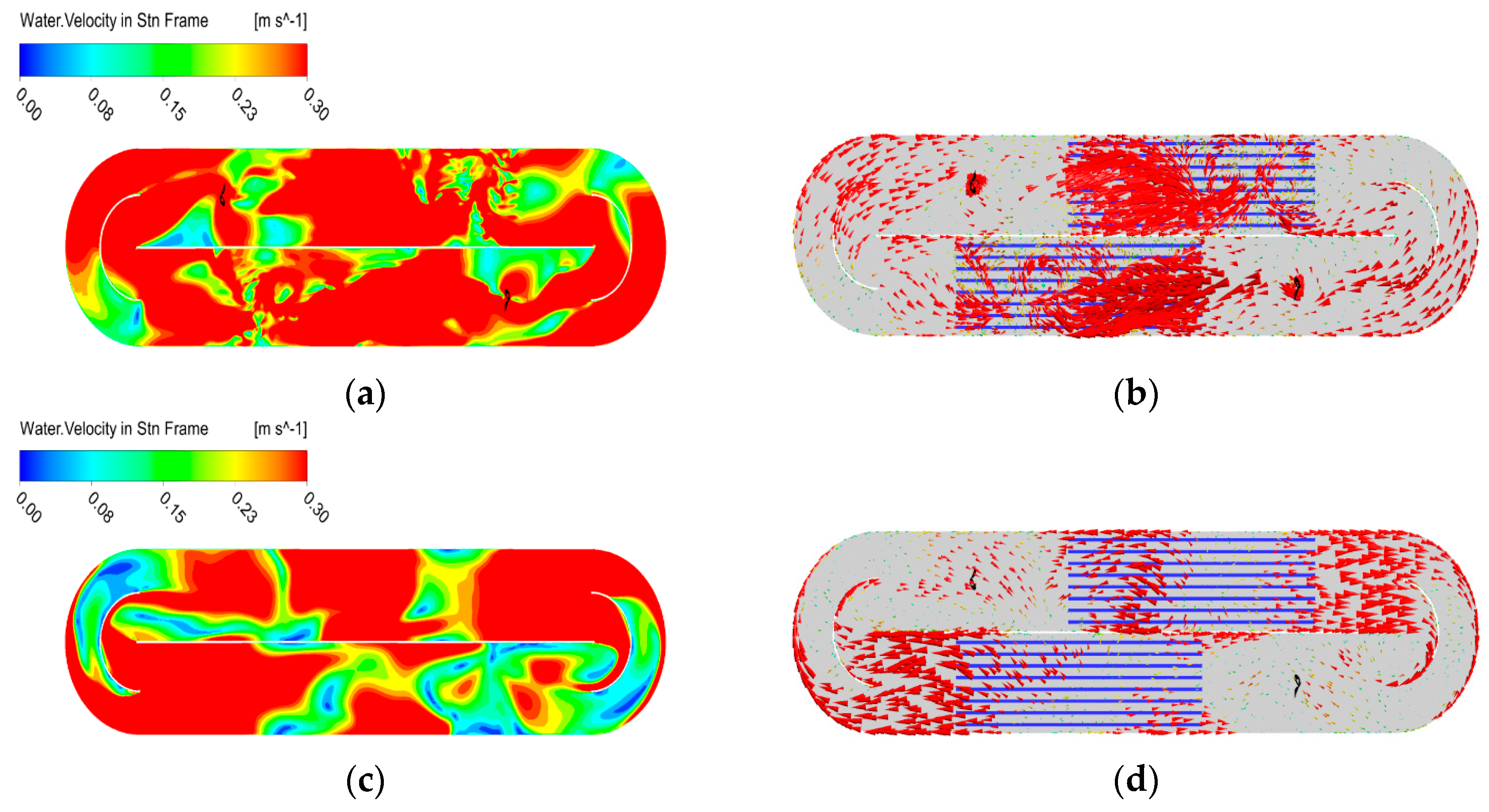
• The momentum source term approach was used due to its reliability and high computing speed. The minimum required liquid velocity was reached with this model and adequate mixing was determined. This approach predicts lower water velocity in comparison with the transient rotor-stator model. This is due to the fact that the tangential velocity components were not considered during flowmaker modelling.
• Despite the excessive computing resource requirements, the transient rotor-stator model accurately predicted the fluid flow pattern in the OD. The flowmakers were able to generate the required thrust in order to obtain sufficient bulk flow. Better mixing performance was determined with this model. Also, the normal forces that act on the blades were monitored and the normal force fluctuations were in the allowed range during the simulation.
• Grundfos best practice guidelines were taken into account for the correct positioning of the flowmakers. Higher thrust fluctuations were determined when the flowmaker position was close to the first row of the diffuser grid. Meanwhile, the uneven distribution of water velocity was observed due to the tank curves and it might be dangerous for the blades. Therefore, the rear clearance is also an important parameter for the correct positioning of the flowmakers. When the distance between the flowmaker and the diffuser grid was 9.96 m, relatively low thrust fluctuations were monitored. As a result, it is the recommended position of the flowmaker for this study.
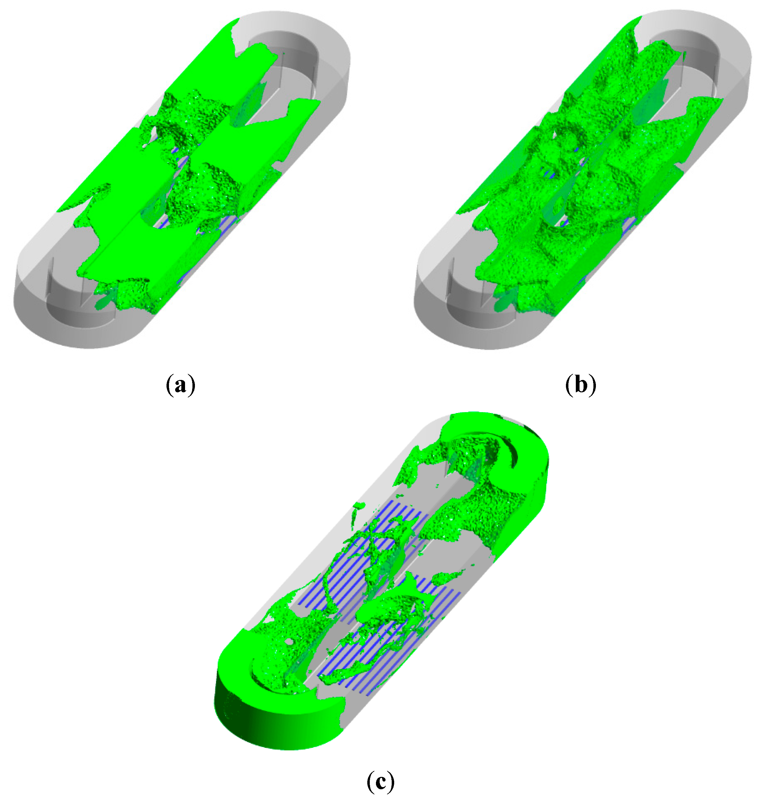
• The contribution of the aeration process to the mixing was also investigated by removing the flowmakers. Inadequate mixing was monitored throughout the OD due to the recirculation zones. Zones of recirculation were determined due to the high aeration rate. There were dead zones around the rounded ends of the oxidation ditch. Also, the diffuser grid arrangement was not suitable to get adequate mixing without the flowmakers. Therefore, it is necessary to use the flowmaker in order to achieve effective bulk flow.
• Fine bubble diffusers were used instead of the more energy-intensive surface aerators and approximately 57% reduction of energy consumption was achieved in the aeration process.

References

1. Grady, L. Daigger and Lim, Biological Wastewater Treatment., 2nd ed.; Marcel Dekker: New York, NY, USA, 1999. [Google Scholar]
2. Fayolle, Y.; Arnaud, C.; Sylvie, G.; Michel, R.; Alain, H. Oxygen transfer prediction in aeration tanks using CFD. Chem. Eng. Sci. 2007, 62, 7163–7171. [Google Scholar] [CrossRef]
3. Karpinska, A.M.; John, B. CFD-aided modelling of activated sludge systems—A critical review. Water Res. 2015, 88, 861–879. [Google Scholar] [CrossRef] [PubMed] [Green Version]
4. Tchobanoglous, G.; Burton, F.L.; Stensel, H.D.; Metcalf & Eddy, Inc. Wastewater Engineering: Treatment and Reuse, 4th ed.; McGraw-Hill: New York, NY, USA, 2003. [Google Scholar]
5. Grundfos, Fixed Bottom Aeration Grid and Agitators. Available online: https://www.grundfos.com/ (accessed on 27 March 2020).
6. Rosa, L.M.; Koerich, D.M.; Giustina, S.V. The Use of CFD in Design and Optimization of Wastewater Treatment Units: A Review. 2017. Available online: https://www.researchgate.net/publication/317771587_The_use_of_CFD_in_design_and_optimization_of_wastewater_treatment_units_A_review (accessed on 10 January 2020).
7. Yang, Y.; Yang, J.; Zuo, J.; Li, Y.; He, S.; Yang, X.; Zhang, K. Study on two operating conditions of a full-scale oxidation ditch for optimization of energy consumption and effluent quality by using CFD model. Water Res. 2011, 45, 3439–3452. [Google Scholar] [CrossRef] [PubMed]
8. Motivation and Strategy, “www.hzdr.de” HZDR-WebCMS, 21 August 2019. Available online: https://www.hzdr.de/db/Cms?pOid=50658&pNid=121 (accessed on 28 February 2020).
9. Climent, J.; Martinez-Cuenca, R.; Carratala, P.; Gonzalez-Ortega, M.J.; Abellan, M.; Monros, G.; Chiva, S. A comprehensive hydrodynamic analysis of a full-scale oxidation ditch using Population Balance Modelling in CFD simulation. Chem. Eng. J. 2019, 374, 760–775. [Google Scholar] [CrossRef]
10. Vermande, S.; Essemiani, K.; Meinhold, J.; Traversay, C.D.; Fonande, C. Trouble shooting of agitation in an oxidation ditch: Applicability of hydraulic modeling. In Proceedings of the 76th Annual Technical Exhibition and Conference WEFTEC’03, Los Angeles, CA, USA, 11–15 October 2003. [Google Scholar]
11. Xie, H.; Yang, J.; Hu, Y.; Zhang, H.; Yang, Y.; Zhang, K.; Zhu, X.; Li, Y.; Yang, C. Simulation of flow field and sludge settling in a full-scale oxidation ditch by using a two-phase flow CFD model. Chem. Eng. Sci. 2014, 109, 296–305. [Google Scholar] [CrossRef]
12. Stamou, A.I. Prediction of hydrodynamic characteristics of oxidation ditches using the k-e turbulence model. In Proceedings of the Second International Symposium on Engineering Turbulence Modelling and Measurements, Florence, Italy, 31 May–2 June 1993. [Google Scholar]
13. Karcz, J.; Kacperski, L. An effect of the grid quality on the result of numerical simulations of the fluid flow field in an agitated vessel. In Proceedings of the 14th European Conference on Mixing, Warszawa, Poland, 10–13 September 2012. [Google Scholar]
14. Brannock, M. Computational Fluid Dynamics Tools for the Design of Mixed Anoxic Wastewater Treatment Vessels. Ph.D. Thesis, Department of Environmental Engineering, University of Queensland, Brisbane, Australia, 2003. [Google Scholar]
15. ANSYS CFX-Solver Modeling Guide; ANSYS Inc.: Canonsburg, PA, USA, 2009.
16. Andersson, B.; Andersson, R.; Hakansson, L.; Mortensen, M.; Sudiyo, R.; Van Wachem, B. Computational Fluid Dynamics for Engineers; Cambridge University Press: New York, NY, USA, 2012. [Google Scholar]
17. Ratkovich, N. Understanding Hydrodynamics in Membrane Bioreactor Systems for Wastewater Treatment: Two-phase Empirical and Numerical Modelling and Experimental Validation. Ph.D. Thesis, Ghent University, Belgium, Ghent, 2010. [Google Scholar]
18. Ishii, M.; Zuber, N. Drag Coefficient and Relative Velocity in Bubbly, Droplet or Particulate Flows. AIChE J. 1979, 25, 843–855. [Google Scholar] [CrossRef]
19. Dean, J.A. Lange–s Handbook of Chemistry, 15th ed.; McGraw-Hill: New York, NY, USA, 1999. [Google Scholar]
20. Burns, A.D.; Frank, T.; Hamill, I.; Shi, J.-M. The Favre Averaged Drag Model for Turbulent Dispersion in Eulerian Multi-Phase Flows. In Proceedings of the 5th International Conference on Multiphase Flow, Yokohama, Japan, 30 May–4 June 2004. [Google Scholar]
21. Karpinska, A.M.; Bridgeman, J. CFD as a tool to optimize aeration tank design and operation. J. Environ. Eng. 2018, 144, 05017008. [Google Scholar] [CrossRef]
22. Menter, F.R. Two-Equation Eddy-Viscosity Turbulence Models for Engineering Applications. AIAA J. 1994, 32, 1598–1605. [Google Scholar] [CrossRef] [Green Version]
23. Grundfos, “Design Recommendations for Mixing,” 2014. Available online: https://www.grundfos.com/campaigns/download-mixer-handbook.html (accessed on 26 March 2020).
Figure 1. Fixed bottom aeration grid and agitators [5].
Energies 13 01633 g001
Figure 2. 3D view of the full-scale oxidation ditch, agitators (1 and 2), diffuser grids (3 and 4).
Energies 13 01633 g002
Figure 3. Comparison of Air Volume Fraction.
Energies 13 01633 g003
Figure 4. Water velocity contour (a,c) and its vectorial representation (b,d) on a horizontal plane at 0.5 m and 6 m (from top to bottom) above the tank floor.
Energies 13 01633 g004
Figure 5. Water velocity streamlines (a) and average water velocity plot (b).
Energies 13 01633 g005
Figure 6. Air volume fraction isosurface (a) and air holdup plot (b).
Energies 13 01633 g006
Figure 7. Water velocity contour (a,c) and water velocity vectors (b,d) on a horizontal plane at 0.5 m and 6 m (from top to bottom) above the tank floor.
Energies 13 01633 g007
Figure 8. Water velocity plot (a) and air holdup plot (b).
Energies 13 01633 g008
Figure 9. Normal force on the blades of the flowmakers in axial (Z) and radial (X and Y) directions.
Energies 13 01633 g009
Figure 10. Normal force on the blades in axial (Z) and radial (X and Y) directions after stopping the flowmakers.
Energies 13 01633 g010
Figure 11. Oxidation ditch plan for Case 1 (a) and Case 2 (b).
Energies 13 01633 g011
Figure 12. Normal force plots of flowmaker 1 for Case 1 (orange) and Case 2 (green).
Energies 13 01633 g012
Figure 13. Water velocity contour (a,c) and water velocity vectors (b,d) on a horizontal plane at 0.5 and 6 m (from top to bottom) above the tank floor.
Energies 13 01633 g013
Figure 14. Water velocity isovolumes, (a) above 0.3 m/s; (b) 0.3 m/s; (c) below 0.1 m/s.
Energies 13 01633 g014