Viscosity Loss and Hydraulic Pressure Drop on Multilayer Separate Polymer Injection in Concentric Dual-Tubing

Abstract

Multilayer separate polymer injection in concentric dual-tubing is a special method for enhancing oil recovery in later development stage of the multilayer formation. During the injection process, heat exchange occurs among the inner tubing, tubing annulus and formation, making the thermal transfer process more complicated than traditional one. This work focuses on the polymer flowing characteristics during the multilayer separate polymer flooding injection process in the wellbore. A temperature–viscosity numerical model is derived to investigate the influencing factors on polymer dual-tubing injection process. Then, an estimate-correct method is introduced to derive the numerical solutions. Several influences have been discussed, including the axial temperature distribution, viscosity distribution, pressure drop, and flow pattern of polymer. Results show that under low injecting rates, below 5 m³/d, formation temperature will greatly decrease the polymer viscosity. When the injecting rates above 20 m³/d, the polymer just decreases 1–3 mPa·s at the bottom of well, which is really small. Additionally, the temperature distribution, the coefficient of friction under different injecting rates have been discussed. Generally, this method provides a new way to analyze thermal conductivity during the polymer injection process which is meaningful for polymer flooding in the oilfield application.

1. Introduction

In the past decades, polymer flooding has gradually become an effective method to enhance oil recovery (EOR) [1,2,3]. In Daqing oil field, which is the largest oil field in China, polymer flooding has contributed to more than 10 % of enhanced oil recovery [4,5], and over ten million tons of crude oil has been produced every year by polymer flooding [6,7]. Nowadays, alkali-surfactant-polymer (ASP) combinational flooding system has become a promising direction of EOR technology [8,9,10]. It was proved that the ASP flooding has improved oil recovery by 17.2% and recovery increment of SP flooding can reach 14.3% [11]. Despite the existing challenges, many researchers have studied the advances and technological method for polymer flooding in heavy oil reservoir [12,13,14] and the field application shows that the polymer flooding of heavy oils could result in incremental recoveries ranging from 7.5 to 25% OOIP [15]. Moreover, due to high demand for energy, polymer flooding has been successfully applied in offshore oil production in China [16,17,18,19]. As the development of the oil field, the main objectives of polymer flooding turns into type Ⅱ formation, which has strong vertical heterogeneity between layers, and the physical properties between the high-permeability and low-permeability layer differ greatly [20,21,22]. Currently, under the low oil price, more recovery efficiency of polymer flooding is required, not only for the heterogeneous reservoir development, but also for heavy oil and offshore polymer flooding. According to this demand, multilayer separate polymer injection technology has been fully developed and applied.

The multilayer separate injection technology has two main ways. One is using allocators for different oil layers, as shown in Figure 1. However, this method has an obvious shortcoming that the flow channel, which is only 1 mm, is easily blocked by tiny impurities in polymer solution. For another method, the concentric dual-tubing injection is adopted as shown in Figure 2. Inner tubing injection for lower formation, and annulus injection between concentric tubing is for the upper oil layer. This method has been widely used in onshore and offshore oil fields and proved increasing oil recovery efficiency [23]. Research on dual-tubing injection of multilayer separate polymer flooding is meaningful to field application.

In polymer flooding, polymers are injected from injecting wells, and then the residual oil is displaced in the reservoir. As such, the method is more complicated than conventional water injection [24,25,26]. Two EOR mechanisms are available for polymer flooding. The first one is micro displacement efficiency enhancement, and the other is flooding volume increment [27,28]. The effectivity of these two mechanisms is mainly influenced by polymer viscosity. Viscosity is the key factor in the oil recovery. The higher the viscosity, the better the displacement effect. Studies have shown that the polymer solution is non-Newtonian power-law fluid, and its apparent viscosity is greatly influenced by shear stress and temperature [29,30,31]. The polymer is heated up by formation as the formation temperature increases with depth. Thus, the polymer viscosity decreases, and related friction and pressure drop will also change. The key to understanding the polymer viscosity change, hydraulic friction, and pressure loss during the dual-tubing injection process is to derive the variation of the polymer’s temperature in the wellbore.

Temperature calculation, along with wellbore trajectory, is a classic approach widely used to solve various problems, such as steam injection, geothermal heating from the abandoned oil wells, polymer injection, and other engineering applications [32,33,34,35]. The downhole heat transfer is a relatively strong nonlinear process [36,37]. As injected liquid heated up, many heat transfer parameters are changing, including the viscosity, flow pattern, heat conductivity, pressure loss, etc. The numerical method is commonly used to solve this problem, like estimate-correct method. In this method, the wellbore is segmented into several units. In each unit, the physical characteristic of the liquid is considered stable. Several parameters, such as thermal conductivity and flow pattern, can be calculated by estimating the average temperature. The calculated temperature can be derived on the basis of these results. If the estimated temperature approaches the calculated one, then the real temperature can be derived. Several studies have been conducted using this method [38]. Livescu and Wand proposed a temperature-dependent coefficient of friction correction and implemented the correction into a tubing and annulus circulation model to study the downhole temperature distribution [34]. Yi et al. coupled the transient temperature and pressure in carbon dioxide injection well, and solved the thermal equation by discretization method. Wei et al. extended the model by introducing multiphase flow in downhole [39]. For polymer injection in separated formation layers, the key is to understand the heat transfer between the inner and outer tubing. Sun et al. [40] investigated the teat transfer process between the inner and outer tubing in steam injection. Similarly, the method can be introduced into the polymer injecting process. In a separate layer injection, polymer 1 was injected into the inner tubing, whereas polymer 2 was injected into the annulus between the inner and outer tubing. Thus, the thermal behavior of polymer in the concentric annulus should be investigated. Batra and Sudarsan [41] developed a numerical model to study the heat transfer process in an annular channel. However, the fluid is Newtonian liquid. Pinho and Coelho [42] studied the thermal behavior of viscoelastic fluids with viscous dissipation. Allanic et al. [43] provided a numerical model to predict the velocity profile of the polymer under steady conditions in the annulus. Li and Delshad [44] introduced a thermal-viscosity coupling model into reservoir simulation, and achieved an economic injecting rate for polymer solutions. However, during multilayer separate polymer injection, the heat transfer between concentric dual-tubing, and related temperature-viscosity coupling in injection process are not well studied, which is an important problem in the polymer injection process in oilfields.

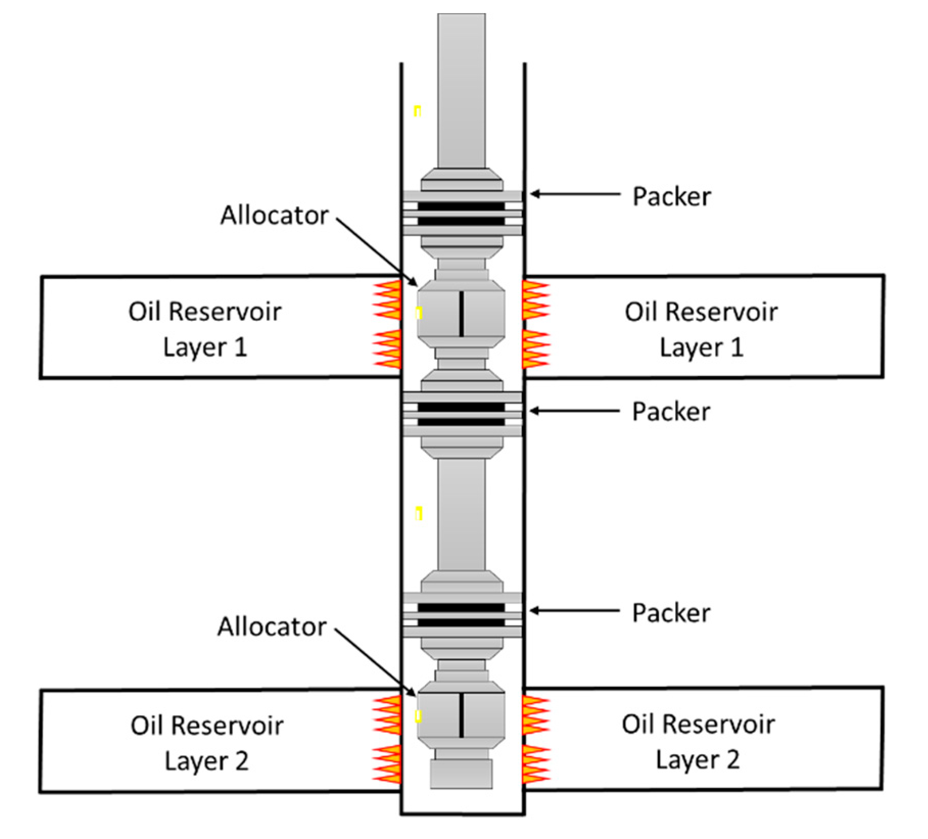
2. Downhole Polymer Injection Process

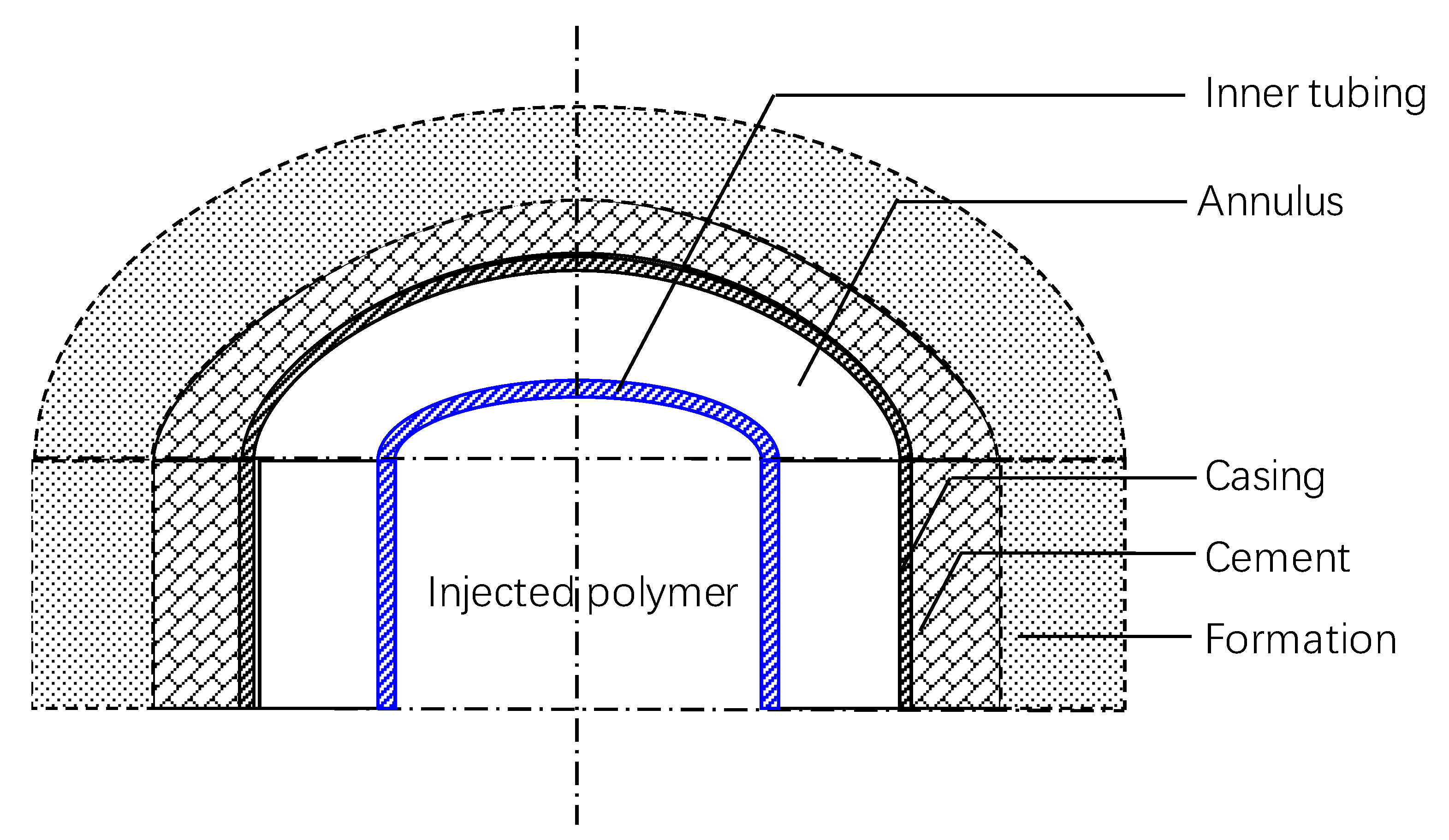
2.1. Model Description

Commonly, the polymer is injected through wellbore. The structure of a classic wellbore is shown in Figure 3. This is a classical heat transfer problem in concentric dual-tubing and formation. In Figure 3, six annular layers are present from the inner tubing to the formation, including the inner tubing, insulation, outer tubing, annulus, casting, and formation. During the polymer injection process, the temperature of the injected polymer is different from that of formation. Thus, thermal transfer occurs between the injected polymer and formation. For multilayer separate polymer injection well by concentric dual-tubing, there are two layers of tubing, shown in Figure 4. The outer tubing is marked red, which is different from single tubing injecting in Figure 3. The polymer in the inner tubing is injected into the lower formation, whereas the polymer in the annulus between the inner and outer tubing is injected into the upper formation. The tubing–casing annulus is filled with a static polymer during the polymer injection process.

2.2. Solution of General Heat Transfer Equation

The heat transfer process in the radial system is a classic problem. The temperature of the injected liquid is different from that of the formation. Thus, heat transfer occurs between the injected liquid and formation. Heat transfer for the separated layer polymer injection in a double tubing is complicated and occurs in three parts. The first part is the heat transfer from the polymer in the inner tubing to that in the outer tubing. The second part is the heat transfer from the polymer in the outer tubing to the annulus. The third part is the heat transfer from the polymer in the annulus to the formation. The governing equation of heat transfer in the cylindrical coordinates in the formation is as follows:

$$(\frac{1}{r}\frac{\partial }{\partial r}\left(r\frac{\partial T}{\partial r}\right)=\frac{1}{a}\frac{\partial T}{\partial \tau }\tau >0,r_h<r<\infty ).$$

(1)

where $T$ is the formation temperature, $r$ is radial distance from the center of the wellbore, $r_h$ is the outside radius of the wellbore, commonly represented as the interface between cement and formation. $\tau$ is the injection time, $a$ is thermal diffusion coefficient of the formation. The initial condition can be expressed as follows:

$$T{|}_{\tau =0}=T_{ez}$$

(2)

where $T_{ez}$ is the initial temperature of the formation at the depth of the middle point in the calculation unit, which can be expressed as follows:

$$T_{ez}=T_s+mz.$$

(3)

where $T_s$ is the temperature at the surface, $m$ is the geothermal gradient, $z$ is the depth of the middle point of the calculation unit. The inner and outer boundary conditions can be expressed as follows:

$${-2\pi \lambda \left(r\frac{\partial T}{\partial r}\right)|}_{r=r_h}=q_{lz},T{|}_{r\to \infty }=T_{ez}$$

(4)

where $\lambda$ is overall thermal conductivity, $q_{lz}$ is the amount of heat transferred from wellbore to formation in unit length. The analytical solution of Equation (1) can be expressed by combining Equations (1) to (4).

$$\begin{gathered} T(r,\tau )=T_{ez}+\frac{q_{lz}}{{\pi }^2\lambda }I, \\ \mathrm{where}I={\displaystyle {\int }_0^{\infty }\frac{1-\exp \left(-a\tau u/r_h^2\right)}{u^2}\times \frac{Y_1\left(u\right)J_0\left(ru/r_h^{}\right)-J_1\left(u\right)Y_0\left(ru/r_h^{}\right)}{J_1^2\left(u\right)+Y_1^2\left(u\right)}}du \end{gathered}$$

(5)

where $J_0$ and $J_1$ are the first kind zero-order Bessel function and the first kind first-order Bessel function, respectively; $Y_0$ and $Y_1$ are the second kind zero-order Bessel function and the second kind first-order Bessel function, respectively. We can derive the temperature at the cement and formation interface by setting $r=r_h$.

$$T_{r_h}=T(r_h,\tau )=T_{ez}+\frac{q_{lz}}{{\pi }^2\lambda }I\left(r_h,\tau \right)=f\left(\tau \right),$$

(6)

where $I={\displaystyle {\int }_0^{\infty }\frac{1-\exp \left(-a\tau u/r_h^2\right)}{u^2}\times \frac{Y_1\left(u\right)J_0\left(u\right)-J_1\left(u\right)Y_0\left(u\right)}{J_1^2\left(u\right)+Y_1^2\left(u\right)}}du$. Equation (5) can be simplified by defining dimensionless temperature $T_D=-(T_{r_h}-T_{ez})\times {(\frac{q_{lz}}{2\pi \lambda })}^{-1}$ and dimensionless time ${\tau }_D=a\tau /r_h^2$.

$$T_D=-\frac{2}{\pi }I$$

(7)

Hasan and Kabir [45] provided the approximate numerical solution of Equation (7), which can be expressed as follows:

$$T_D=\{\begin{array}{cc}1.1281\sqrt{{\tau }_D}(1-0.3\sqrt{{\tau }_D})& ({\tau }_D\le 1.5)\hfill \\ (0.4063+0.5\ln {\tau }_D)\left(1+\frac{0.6}{{\tau }_D}\right)& ({\tau }_D>1.5)\hfill \end{array}$$

(8)

Equation (8) provides an accurate and efficient way to express the variation of temperature with time at the cement and formation interface, which is significant for the heat transfer calculation of injected polymers.

2.3. Heat Transfer in and out of the Wellbore

The heat transfer process in the wellbore is complicated. The key is to determine the heat transfer coefficient. However, this parameter is influenced by the liquid flowing behavior, which is controlled by flowing velocity, viscosity, and temperature. Hence, the estimate-correct method should be introduced in the calculation process. A detailed process is discussed in the later parts. As previously shown, the polymer injection method is divided into two types. The first one is normal single tubing injection, and the second one is separated double tubing injection. Figure 1 and Figure 2 present the schematic of these methods. We generally introduce the second method in the following process because the first method is traditional and has been investigated by several previous studies.

During the separated double tubing injection process, the polymer in the inner and outer tubing may vary in behavior in terms of injection velocity, temperature, viscosity, and flowing pattern. Heat transfer is generally forced convection. The annulus is commonly filled with static liquid, thus it is a free convection heat transfer process.

We focus on a separated unit, such as the depth from $z1$ to $z2$, in the Z-direction to analyze the heat transfer process. In this unit, the parameters remain constant even though the depth increases. The relationship between thermal resistance and the amount of transferred heat from the inner to the outer tubing $q_{l1}$ can be expressed as follows:

$$q_{l1}=\frac{T_{f1}-T_{r3}}{R_1}$$

(9)

where $T_{f1}$ is the temperature of liquid in inner tubing (liquid 1). $T_{to}$ is the temperature of liquid 2 (injected polymer between inner tubing and outer tubing) at interface $r_3$. $R_1$ is the thermal residence within the tubing and can be expressed as follows:

$$R_1=\frac{1}{2\pi r_{ti}{h}_{f1}}+\frac{1}{2\pi {\lambda }_{steel}}\ln \left(\frac{r_2}{r_{ti}}\right)+\frac{1}{2\pi r_2{h}_{f2}}+\frac{1}{2\pi {\lambda }_{steel}}\ln \left(\frac{r_{to}}{r_3}\right)$$

(10)

where $h_{f1}$ and $h_{f2}$ are forced-convection heat transfer coefficient for liquid 1 and liquid 2. ${\lambda }_{steel}$ is the thermal conductivity of steel. $r_{ti}$ is inner radius of inner tubing, $r_2$ is outer radius of inner tubing, $r_3$ is the inner radius of outer tubing, $r_{to}$ is the outer radius of outer tubing. The amount of transferred heat $q_{l2}$ out of the tubing can be expressed as follows:

$$q_{l2}=\frac{T_{to}-T_h}{R_2}$$

(11)

where $T_{to}$ is the temperature of static liquid in annulus (liquid 3) at interface $r_{to}$, $T_h$ is the temperature at cement-formation interface. $R_2$ is the thermal residence from the outer tubing to the cement–formation interface and can be expressed as follows:

$$R_2=\frac{1}{2\pi r_{to}{h}_{f3}}+\frac{1}{2\pi {\lambda }_{steel}}\ln \left(\frac{r_{co}}{r_{ci}}\right)+\frac{1}{2\pi {\lambda }_{cem}}\ln \left(\frac{r_h}{r_{co}}\right)$$

(12)

where $h_{f3}$ is the natural-convection heat transfer coefficient for liquid 3. $r_{ci}$ and $r_{co}$ are inner and outer radius of casing, $r_h$ is the radius of cement-formation interface. ${\lambda }_{cem}$ is the thermal conductivity of cement.

Considering that the thermal conductivity of steel is much larger than that of liquid, we ignore the temperature loss within the steel; thus, heat resistance with the ${\lambda }_{steel}$ term is ignored. Liquid 1 is mixed from pump, and the viscosity is commonly high. Accordingly, the liquid temperature $T_{f1}$ is considered uniform. Thus, the item with $h_{f1}$ is ignored, indicating that the inner heat transfer of liquid 1 is ignored. Finally, $R_1$ and $R_2$ are simplified as follows:

$$R_1=\frac{1}{2\pi r_2{h}_{f2}},R_2=\frac{1}{2\pi r_{to}{h}_{f3}}+\frac{1}{2\pi {\lambda }_{cem}}\ln \left(\frac{r_h}{r_{co}}\right)$$

(13)

The temperature is simplified as follows:

$$T_{r3}=T_{to},T_{r2}=T_{ti},T_{ci}=T_{co}$$

(14)

The inner and outer tubing are regarded as virtual equivalent tubing with a range within $r_{to}$ to simplify the analytical process. The heat transfer out of equivalent tubing is $q_{l2}$, and the amount of transferred heat from the inner to outer tubing $q_{l1}$ is regarded as the inner heat transfer. The general heat transfer equation for equivalent tubing can be also expressed as follows:

$$q_{l2}=2\pi r_{to}{k}_{to}(T_{to}-T_h)$$

(15)

where $k_{to}$ is the overall heat-transfer coefficient based on $r_{to}$. The following expression can be derived by combining Equations (11)–(15).

$$k_{to}={\left[\frac{1}{h_{f3}}+\frac{r_{to}}{{\lambda }_{cem}}\ln \left(\frac{r_h}{r_{co}}\right)\right]}^{-1}$$

(16)

As previously illustrated, liquids 1 and 2 are force-injected in the formation, whereas liquid 3 is static. Thus, the heat transfer for liquids 1 and 2 is forced convection, whereas that for liquid 3 is natural convection.

For liquid 3, in annulus space between $r_{to}$ and $r_{ci}$, the amount of transferred heat, $q_c$ can be expressed as follows:

$$q_c=2\pi r_{to}{h}_{f3}(T_{to}-T_{ci})$$

(17)

An equivalent thermal conductivity for static liquid ${\lambda }_{f3}$ can be introduced to calculate the free-convective heat transfer coefficient $h_{f3}$.

$$q_c=2\pi {\lambda }_{f3}\frac{T_{to}-T_{ci}}{\ln (r_{ci}/r_{to})}$$

(18)

The following heat transfer coefficient for natural convection is obtained by combining the above-mentioned two equations:

$$h_{f3}={\lambda }_{f3}{\left(r_{to}\ln \frac{r_{ci}}{r_{to}}\right)}^{-1}$$

(19)

where ${\lambda }_{f3}$ can be expressed as follows [46]:

$${\lambda }_{f3}=\{\begin{array}{cc}{\lambda }_a& (Ra\le 6000)\\ \left(2+0.5R{a}^{1/4}\right){\lambda }_a& (6000<Ra\le {10}^6)\\ 0.046{\lambda }_{a}R{a}^{1/3}& ({10}^6<Ra\le {10}^9)\end{array}$$

(20)

Parameter $Ra$ can be expressed as follows:

$$\begin{array}{cc}\hfill Ra& =Gr\mathrm{Pr}=\left[\frac{{\left(r_{ci}-r_{to}\right)}^3\left(T_{to}-T_{ci}\right)g{\alpha }_V{\rho }^2}{{\eta }^2}\right]\left(\frac{c_p\eta }{{\lambda }_a}\right)\hfill \\ & =\left(\frac{g{\alpha }_V{\rho }^2{c}_p}{\eta {\lambda }_a}\right){\left(r_{ci}-r_{to}\right)}^3\left(T_{to}-T_{ci}\right)\hfill \end{array}$$

(21)

where $Ra$ is Rayleigh number, $Gr$ is Grashof number, $\mathrm{Pr}$ is Prandtl number, $g$ is acceleration due to Earth’s gravity, $a_v$ is coefficient of thermal expansion, $\rho$ is fluid density, $c_p$ is specific heat for liquid, $\eta$ is kinematic viscosity, ${\lambda }_a$ is thermal conductivity. The free-convective heat transfer coefficient $h_{f3}$ can be determined by combining Equations 15–21.

For liquid 2, in annulus space between $r_3$ and $r_2$, the amount of transferred heat is $q_{l1}$, which has been expressed before. In heat transfer process, the key is to determine the force-convective heat transfer coefficient $h_{f2}$. In annulus space, Nusselt number $Nu$ is introduced to calculate $h_{f2}$. The definition of $Nu$ in liquid 2 is

$$Nu=\frac{h_f}{{\lambda }_f}{d}_e$$

(22)

where ${\lambda }_{f2}$ is the thermal conductivity of the fluid 2. $d_e$ is characteristic length. For annulus space, $d_e=2(r_3-r_2)$. The Nusselt number $Nu$ is influenced by flow pattern. For laminar flow, $Nu$ can be expressed as [46]:

$$Nu=4.36$$

(23)

For transitional flow and turbulent flow, $Nu$ can be expressed as [46]:

$$Nu=\{\begin{array}{cc}0.0214\left({\mathrm{Re}}^{0.8}-100\right){\mathrm{Pr}}^{0.4}\hfill & 0.5<\mathrm{Pr}<1.5,{10}^4<\mathrm{Re}<5\times {10}^6\\ 0.012\left({\mathrm{Re}}^{0.87}-280\right){\mathrm{Pr}}^{0.4}\hfill & 1.5<\mathrm{Pr}<500,3000<\mathrm{Re}<{10}^6\end{array}$$

(24)

where $\mathrm{Re}$ is Reynolds number. During polymer injection in the annular space, $\mathrm{Re}$ is

$$\mathrm{Re}=\frac{{12}^{1-n}{\left(2r_3-2r_2\right)}^n\rho v^{2-n}}{C}{\left(\frac{3n}{2n+1}\right)}^n$$

(25)

where $v$ is flowing velocity, $C$ is flow consistency index for polymer, $n$ is flow behavior index for power-law polymer. The hydraulic friction and hydraulic pressure drop are as follows:

$$f_a=24/\mathrm{Re}$$

(26)

$$\frac{dp}{dL}=\frac{4C}{(2r_3-2r_2)}{\left[\frac{2n+1}{3n}\frac{12v}{\left(2r_3-2r_2\right)}\right]}^n$$

(27)

The average shear rate of polymer solution on any cross section of the annular space is

$$\overline{\gamma }=\frac{v(3n+1)}{n}{\left[\frac{n{(r_3-r_2)}^2}{2n-1}\right]}^{\frac{1}{n-1}}$$

(28)

During polymer injection in the circular inner tubing, $\mathrm{Re}$ can be expressed as follows:

$$\mathrm{Re}=\frac{8^{1-n}{\left(2r_{ti}\right)}^n\rho v^{2-n}}{C}{\left(\frac{1+3n}{4n}\right)}^n$$

(29)

The related hydraulic friction and hydraulic pressure drop for the inner tubing can be expressed as follows:

$$f_c=16/\mathrm{Re}$$

(30)

$$\frac{dp}{dL}=\frac{4C}{(2r_{ti})}{\left(\frac{8v}{2r_{ti}}\right)}^n{\left(\frac{3n+1}{4n}\right)}^n$$

(31)

The polymer solution average shear rate on any cross section of the inner tubing is expressed as

$$\overline{\gamma }=\frac{v(3n+1)}{n}{\left[\frac{n{r}_{ti}{}^2}{2n-1}\right]}^{\frac{1}{n-1}}$$

(32)

2.4. Temperature Calculation at the Cement–Formation Interface and Inner Surface of the Casing

During the heat transfer process from the cement–formation interface to the formation, the flux can be expressed as follows:

$$q_l=\frac{T_h-T_{ez}}{T_D/\left(2\pi {\lambda }_e\right)}$$

(33)

where $T_h$ is the temperature of cement-formation interface, $T_{ez}$ is the initial formation temperature at depth $(z_1+z_2)/2$, which can be determined by Equation (3). In equivalent tubing, the heat escape from the wellbore side should be equal, that is,

$$q_l=q_{l2}=q_c$$

(34)

The temperature at the cement–formation interface is obtained by combining Equations (15), (33), and (34).

$$T_h=\frac{r_{to}{k}_{to}{T}_D{T}_{to}+{\lambda }_e{T}_e}{r_{to}{k}_{to}{T}_D+{\lambda }_e}$$

(35)

Moreover, the temperature at the inner surface of the casing is obtained by calculating from outside to inside.

$$T_{ci}=T_h+q_{l2}\left(\frac{1}{2\pi {\lambda }_{cem}}\ln \frac{r_h}{r_{co}}\right)$$

(36)

The heat transfer process out of $r_{to}$ (out of equivalent tubing) can be determined by estimating $T_{to}$ and verifying $k_{to}$. The detailed process is discussed in the later part.

2.5. Energy Balance Equation

In wellbore units $z_1$ to $z_2$, the heat flux flowing into a unit is equal to that outside a unit. The energy balance equation for the fluid domain in the inner tubing (within the range of $r_{ti}$ or fluid 1 in unit 1) is

$$\{\begin{array}{c}{\Phi }_{in1}=Q_1{\rho }_1{C}_{p1}{T}_{f1\_in}\\ {\Phi }_{e1}=Q_1{\rho }_1{C}_{p1}{T}_{f1\_out}\\ {\Phi }_{k1}=q_{l1}(z_1-z_2)\\ {\Phi }_{in1}={\Phi }_{out1}={\Phi }_{e1}-{\Phi }_{k1}\end{array}$$

(37)

where ${\Phi }_{in1}$, ${\Phi }_{out1}$, ${\Phi }_{k1}$, and ${\Phi }_{e1}$ are the energy flowing into unit 1 from top face, flowing out of unit 1, flowing through side of unit 1 and flowing out of unit 1 from the undersurface, respectively. $Q_1$, ${\rho }_1$ and $C_{p1}$ are volume flow rate, density, specific heat of liquid 1, respectively. $T_{f1\_in}$ and $T_{f1\_out}$ are the temperature of liquid 1 flowing into unit 1 from top face and out of unit 1 from undersurface. $(T_{f1\_in}+T_{f1\_out})/2=T_{f1}$.

Meanwhile, the energy balance equation for the fluid domain between the inner and outer tubing (within the range between $r_2$ and $r_3$ or fluid 2 in unit 2) is

$$\{\begin{array}{c}{\Phi }_{in2}=Q_2{\rho }_2{C}_{p2}{T}_{f2\_in}\\ {\Phi }_{e2}=Q_2{\rho }_2{C}_{p2}{T}_{f2\_out}\\ {\Phi }_{k2}=(q_{l2}-q_{l1})(z_1-z_2)\\ {\Phi }_{in2}={\Phi }_{out2}={\Phi }_{e2}-{\Phi }_{k2}\end{array}$$

(38)

where ${\Phi }_{in2}$, ${\Phi }_{out2}$, ${\Phi }_{k2}$, and ${\Phi }_{e2}$ are the energy flowing into unit 2 from top face, flowing out of unit 2, flowing through side of unit 2 and flowing out of unit 2 from the undersurface, respectively. $Q_2^{}$, ${\rho }_2$ and $C_{p2}$ are volume flow rate, density, specific heat of liquid 2, respectively. $T_{f2\_in}$ and $T_{f2\_out}$ are the temperature of liquid 2 flowing into unit 2 from top face and out of unit 2 from undersurface. $(T_{f2\_in}+T_{f2\_out})/2=T_{f2}$.

The energy balance equation for the fluid domain in the equivalent tubing (within the range of $r_{to}$, taking liquids 1 and 2 as a whole unit, denoted as unit 3) is

$$\{\begin{array}{c}{\Phi }_{in\_avg}={\Phi }_{in1}+{\Phi }_{in2}=Q_1{\rho }_1{C}_{p1}{T}_{f1\_in}+Q_2{\rho }_2{C}_{p2}{T}_{f2\_in}\\ {\Phi }_{e\_avg}={\Phi }_{e1}+{\Phi }_{e2}=Q_1{\rho }_1{C}_{p1}{T}_{f1\_out}+Q_2{\rho }_2{C}_{p2}{T}_{f2\_out}\\ {\Phi }_{k\_avg}={\Phi }_{k1}+{\Phi }_{k2}=q_{l2}(z_1-z_2)\\ {\Phi }_{in\_avg}={\Phi }_{e\_avg}-{\Phi }_{k\_avg}\end{array}$$

(39)

where ${\Phi }_{in\_avg}$, ${\Phi }_{out\_avg}$, ${\Phi }_{k\_avg}$, and ${\Phi }_{e\_avg}$ are the energy flowing into unit 3 from top face, flowing out of unit 3, flowing through side of unit 3 and flowing out of unit 3 from the undersurface, respectively.

To make the energy equations explicit, the schematic of overall heat and volume flow is shown in Figure 5. In Figure 5a, the inner cylinder indicates the inner tubing, which is the flowing space of liquid 1; the annulus means the space between inner and outer tubing, which is the flowing space of liquid 2. The volume flow direction is vertical and the heat flow direction is horizontal. The energy balance equations are shown in Equations (37) and (38). However, the heat transfer parameters of polymer, like thermal conductivity, is not a constant, which changes with temperature, injecting velocity, and some other parameters. This makes the equations difficult to be solved. To simplify the derivation process of energy equations, we regard the liquids 1 and 2 as a whole unit, shown in Figure 5b. The energy balance equations are shown in Equation (39). During the iteration processes, Equation (39) is first solved to determine the average parameters. Then by solving the Equations (37)–(39), parameters for each fluid can be determined.

2.6. Temperature–Viscosity Relationship for the Polymer

Viscosity is influenced by temperature. A series of theories and experiments have concluded that the temperature–viscosity relationship for the polymer follows the Arrhenius equation (Equation (40)) [29,30,31].

$$\mu =A_s\exp \frac{E_a}{RT}$$

(40)

where $E_a$ is the activation energy (Arrhenius energy) of the viscous flow, $T$ is the temperature of liquid, $\mu$ is the apparent viscosity. As is the pre-exponential factor, and $R$ is the universal gas constant. Commonly, the parameters can be determined by a liner relationship on the log–log coordinate system, that is,

$$\ln \mu =A+\frac{B}{T}$$

(41)

where $A=\ln A_s$ and $B=T^{\ast }=E_a/R$ are the Arrhenius activation temperature [31]. Polymer follows the power-law [47,48], the effective viscosity can be expressed as:

$${\mu }_{\mathrm{eff}}=C{\gamma }^{n-1}$$

(42)

where ${\mu }_{\mathrm{eff}}$ is effective viscosity, $C$ is flow consistency index, $\gamma$ is shear rate, $n$ is flow behavior index. The temperature-influenced flow consistency index can be expressed as follows:

$$C=\frac{e^{A+B/T}}{e^{A+B/T_c}}{C}_{TC}$$

(43)

where $C_{TC}$ is the flow consistency index derived at temperature $T_C$. Equation (41) provided a convenient way to connect the power-law and the Arrhenius equation for polymer solution, which is significant to introduce the influence of temperature into non-Newtonian fluid flow behavior.

3. Solution Methods

Polymer injection is a nonlinear process. The temperature distribution is dynamic, and the viscosity, flowing pattern, and other parameters of liquid are influenced by temperature. The key to derive the hydraulic friction and hydraulic pressure drop is to obtain the temperature distribution in the wellbore. The estimate-correct method is commonly used to solve nonlinear problems in the wellbore. In this method, the wellbore is segmented into several units. In each unit, the liquid parameters are stable. The iteration process is as follows:

(1). Starting from the surface, the first segment is taken, or the unit in the depth between $z1$ and $z2$ is calculated.

(2). The initial formation at depth $(z1+z2)/2$ is calculated, and the temperature at the bottom of the unit is estimated.

(3). The temperature of the liquid and the overall thermal conductivity from $r_{to}$ to $r_h$ are estimated.

(4). The temperature at $r_{to}$ and $r_{ci}$ is calculated to derive the temperature of liquid 3. Thereafter, $h_{f3}$ is calculated.

(5). The derived thermal conductivity from $r_{to}$ to $r_h$ is calculated, and the result from step 3 is compared. If the error is intolerable, then step 3 is repeated, and the overall thermal conductivity is re-estimated; otherwise, the overall thermal conductivity from $r_{to}$ to $r_h$ is determined, and the temperature of liquid 3 is obtained.

(6). The temperature of liquid 1 and the temperature interface at $r_2$ and $r_3$ are calculated. Thereafter, the temperature of liquid 2 is calculated. The temperature of liquid 1 in this step and that of step 3 are compared. If the error is intolerable, step 3 is repeated, and the temperature of liquid 1 is re-estimated; otherwise, the temperature of liquid 1 is determined.

(7). The temperature of liquid 2 and the flowing parameters for liquids 1 and 2 are calculated.

(8). The hydraulic friction, hydraulic pressure drop for liquids 1 and 2, and other concerned parameters at the calculated unit are calculated.

(9). The next unit in depth is taken, the temperature of the outlet is updated as the inlet for the next unit, and step 1 is repeated.

(10). The results are obtained, and the variation of parameters is analyzed with depth.

4. Results and Discussions

4.1. Parameter Combination

In this work, we have introduced the numerical iteration method to derive the temperature distribution in separate layer polymer injection well within concentric tubing. Here we listed the nomenclature and the magnitude of parameters in the following examples in

Table 1. Nomenclature with the magnitude of parameter.

Parameter Name	Symbol (units)	Magnitude
Inside radius of inner tubing	$r_{ti}$ (m)	0.02515
Outside radius of inner tubing	$r_2$ (m)	0.03015
Inside radius of outer tubing	$r_3$ (m)	0.0443
Outside radius of outer tubing	$r_{to}$ (m)	0.0508
Inside radius of casing	$r_{ci}$ (m)	0.082
Outside radius of casing	$r_{co}$ (m)	0.0889
Radius of cement-formation interface	$r_h$ (m)	0.10795
Temperature at surface	$t_s$ (°C)	20
Temperature for injected polymer 1 at surface (in inner tubing)	$T_{inj1}$ (°C)	20
Temperature for injected polymer 2 at surface (in tubing annulus)	$T_{inj2}$ (°C)	20
Geothermal gradient	$m$ (°C/m)	0.03
Thermal conductivity of the formation	${\lambda }_e$ (W/(m.K))	1.72
Thermal conductivity of the cement	${\lambda }_{cem}$ (W/(m.K))	0.35
Diffusion coefficient of the formation	$a$ (m2/s)	7.361 × 10−7
Specific heat of polymer 1	$C_{p1}$ (J/(kg.°C))	4200
Specific heat of polymer 2	$C_{p2}$ (J/(kg.°C))	4210
Density of polymer 1	${\rho }_1$ (kg/m3)	1010
Density of polymer 2	${\rho }_2$ (kg/m3)	1020
Injecting rates for polymer 1	$Q_1 ({\mathrm{m}}^3/\mathrm{d})$	20
Injecting rates for polymer 2	$Q_2 ({\mathrm{m}}^3/\mathrm{d})$	20
Depth unit in Z direction in each iteration	$\mathrm{dz}$ (m)	100
Depth of well	Z(m)	1950
The universal gas constant	$R (\mathrm{J}/(\mathrm{mol}.\mathrm{K}))$	8.134
Activation energy/Arrhenius energy	$E_a (\mathrm{J}/\mathrm{mol})$	10,716.746
Pre-exponential factor	$A_s$ (mPa·s)	0.5597

. The inner tubing is 2–3/8 in, outer tubing is 4 in, casing is 7 in. The polymer type is MO-4000 HPAM, relative molecular mass is 2.02 × 107 mg/mol, and solid content is 91.16%. For rheological property, at 20 °C, the polymer solution flow behavior index n = 0.702 and consistency coefficient C = 101.64 mPa·sⁿ.

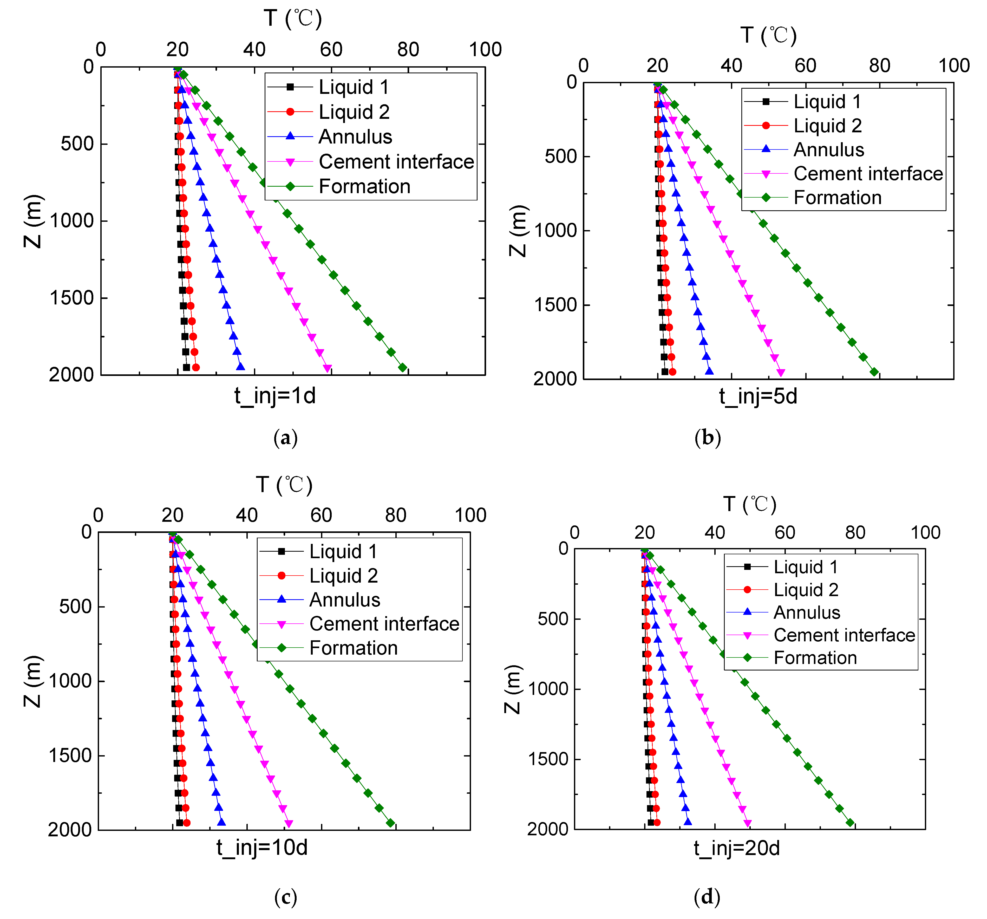
4.2. Temperature Distribution in the Wellbore

Temperature greatly influences the flowing behavior of the injected polymer. The temperature distribution should be derived along with wellbore trajectory. Figure 5 shows the influence of injection rates on the temperature distribution at the total injection time (t = 7 days). The injection rates values in Figure 6a–d are 1, 5, 20, and 50 m³/d, respectively. The reason for choosing these flow rates is that 1 m³/d is the limit flow, which is only used for theoretical analysis; 5 m³/d is selected because the current multi-layered polymer injection is targeted at typeⅡreservoirs, which has relatively low permeability and water absorption capacity, so the injection volume is low. Additionally, 20 and 50 m³/d are the common injection flow rates for separate polymer injection. The injection rates for liquids 1 and 2 are set equally. The calculation process for the unequal situation is the same. We did not discuss such process because it is not our primary concern. The results show that the polymer is warmed up by the formation during the injection process. The temperature in different places in the concentric tubing becomes gradually different in depth within 250 m. Under low injection rates (e.g., 1 m³/d), the liquid temperature linearly increases with depth when the depth is >250 m. Temperature difference among the different layers is stable, indicating that the temperature transfer in the radial direction is stable. The temperature difference among the different layers increases with increasing depth as the injection rates increases. When the injection rates is >20 m³/d, the influence of formation temperature on liquids 1 and 2 is small. Liquids 1 and 2 increase by only several centigrade degrees.

The total injection time also influences the temperature distribution. The heat transfer process from formation to wellbore is an unstable state. The temperature in the near-wall region gradually decreases as the cold polymer is injected in the production layer. Figure 7 shows the variation of temperature distribution as the total injection time increases from 1 day to 20 days under an injection rates of 20 m³/d for both liquid types. The temperature curve for the annulus and cement gradually decreases, whereas the temperature curve for the liquid slightly decreases as the total injection time increases. The injected liquid has no influence on the formation temperature curve within 20 days because it represents the outer boundary of the thermal field (or temperature for the infinite point at a certain depth).

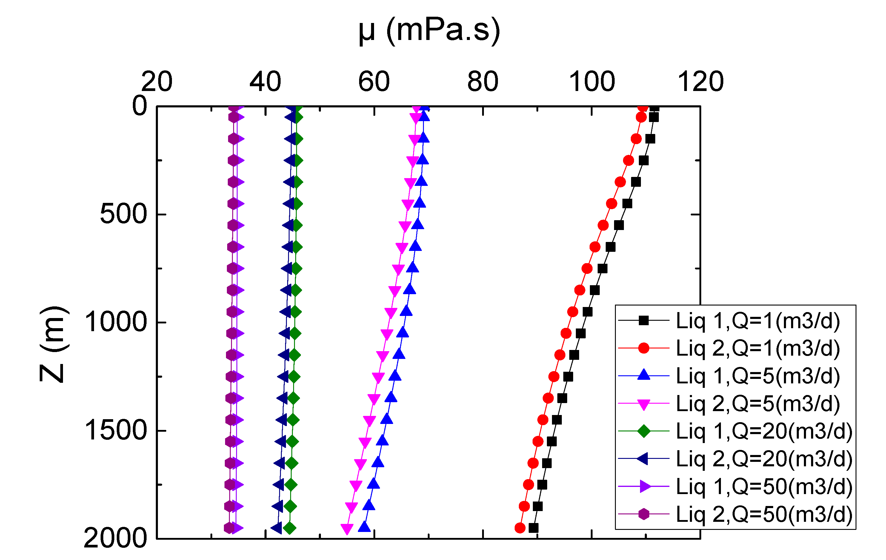
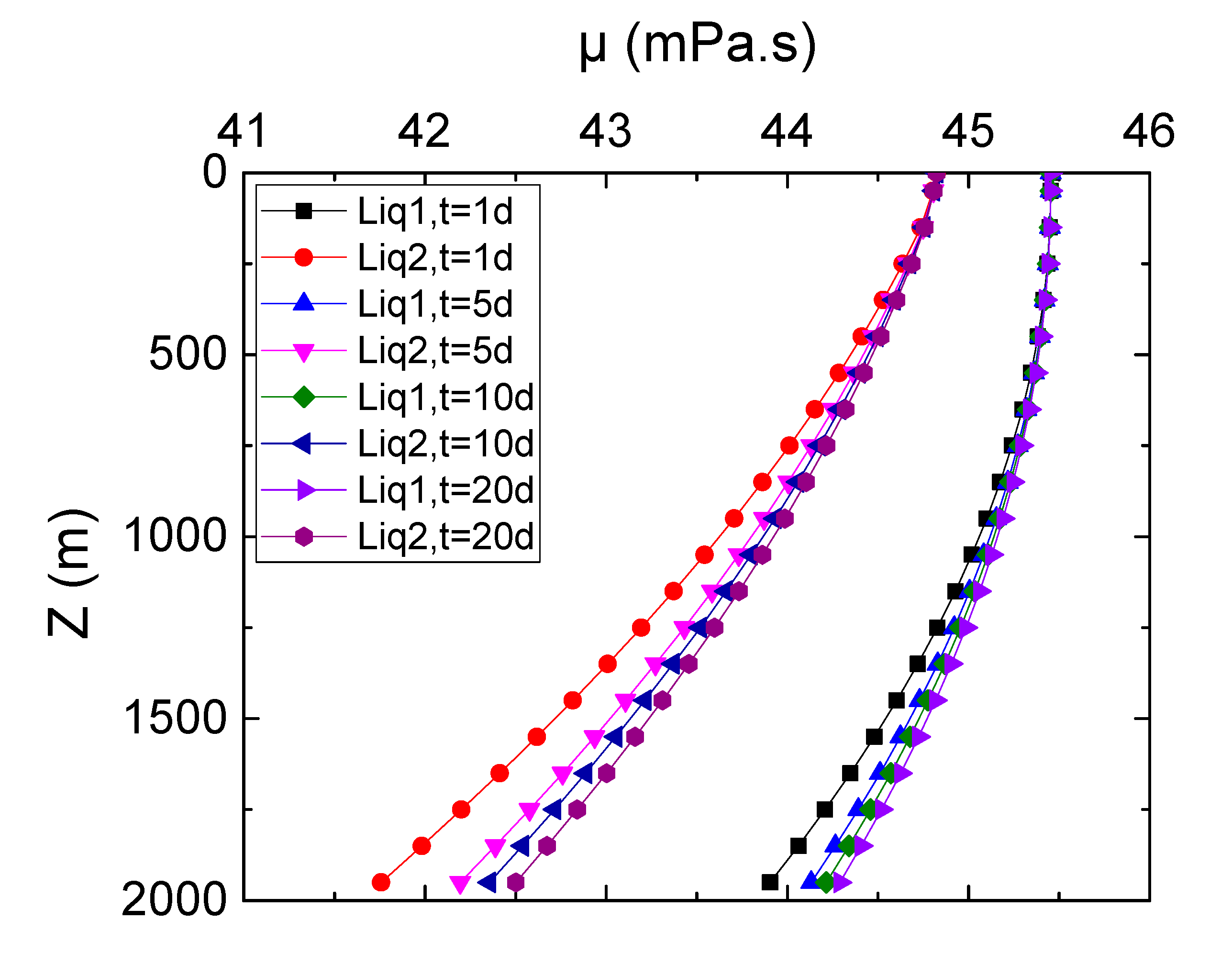
4.3. Average Viscosity Distribution in the Wellbore

During the injection of polymer solution, the viscosity is affected by both shear and temperature. Figure 8 shows the influence of injection rates on viscosity of polymer solution 1 and polymer solution 2 in the whole well section. The injection rates were 1 m³/d, 5 m³/d, 20 m³/d, and 50 m³/d, and the injection time was 7 days. During the polymer injection process, the injection rate is stable, for one kind of injection rate, the flow-dependent shear rate almost does not change during flow in the wellbore. However, different flow rate results in different shear rate. Therefore, in the axial distribution of the injection pipe string, the viscosity affected by the shear action is stable. However, the viscosity of the polymer solution varies in the axial direction due to the influence of temperature. From Figure 8, it can be found that at low flow rates, such as Q = 1 m³/d and Q = 5 m³/d, as the polymer solution is injected into the wellbore, the temperature gradually increases and the viscosity decreases significantly. When the flow rate is 1 m³/d, the viscosity of fluid 1 decreases from 111.6 mPa·s at the wellhead to 89.3 mPa·s at the bottom of the well, and the viscosity of fluid 2 decreases from 109.5 mPa·s to 86.9 mPa·s. When the flow rate is 5 m³/d, the solution viscosity decreases from 69.1 mPa·s to 58.2 mPa·s and 67.8 mPa·s to 54.9 mPa·s, respectively. The solution viscosity is greatly affected by temperature. When the flow rate is 20 m³/d and 50 m³/d, the axial viscosity distribution of the polymer solution is less affected by temperature. The influence of injection rates on viscosity is slight for the injection rates of more than 20 m³/d. The solution viscosity in tubing annulus is more affected by temperature than that in internal tubing. Comparing the polymer solution 1 in the inner tubing with the polymer solution 2 in the annulus of the tubing, it can be seen that the viscosity of the polymer solution 1 is slightly higher than that of the polymer solution 2, but the overall difference is not large.

It can be seen from Figure 8 that shear has the most direct and most significant effect on the viscosity of the polymer solution during injection. At different flow rates, the apparent viscosity of polymer solution varies widely, which is caused by the difference in shear rate. When the flow rate is large, the shear rate is large, and the apparent viscosity of the solution is small. For example, when the injection rate is increased from 1 m³/d to 50 m³/d, the viscosity of fluid 1 is 111.6 mPa·s, 69.1 mPa·s, 45.7 mPa·s, and 34.8 mPa·s respectively, which indicates the viscosity gradually decreases. The viscosity of fluid 2 was 109.5 mPa·s, 67.8 mPa·s, 44.8 mPa·s, and 34.1 mPa·s, respectively. The viscosity also gradually decreases. At the same time, the viscosity of fluid 2 is slightly lower than the viscosity of fluid 1 is also because the solution 2 in the annulus is sheared by both the inner and outer tubing walls.

The total injection time also has a great influence on viscosity distribution. Figure 9 shows the viscosity distribution downhole for liquids 1 and 2 at different total injection times when the injection rates for liquids 1 and 2 are maintained at 20 m³/d. The average velocities of liquids 1 and 2 are different due to the cross-sectional difference for the inner tubing (liquid 1) and annulus between the inner and outer tubing (liquid 2). Thus, the shear rate is different and viscosity of these two liquid types have a slight difference. Figure 9 shows that the viscosity of liquid 2 is slightly lower than that of liquid 1. The viscosity of both liquid types at the bottom of the wellbore increases as the total injection time increases. So, the viscosity loss during the injection process decreases. The influence of injection time on viscosity gradually decreases as the total injection time increases. However, compared with the influence of injecting rates, the influence of injecting time is weaker.

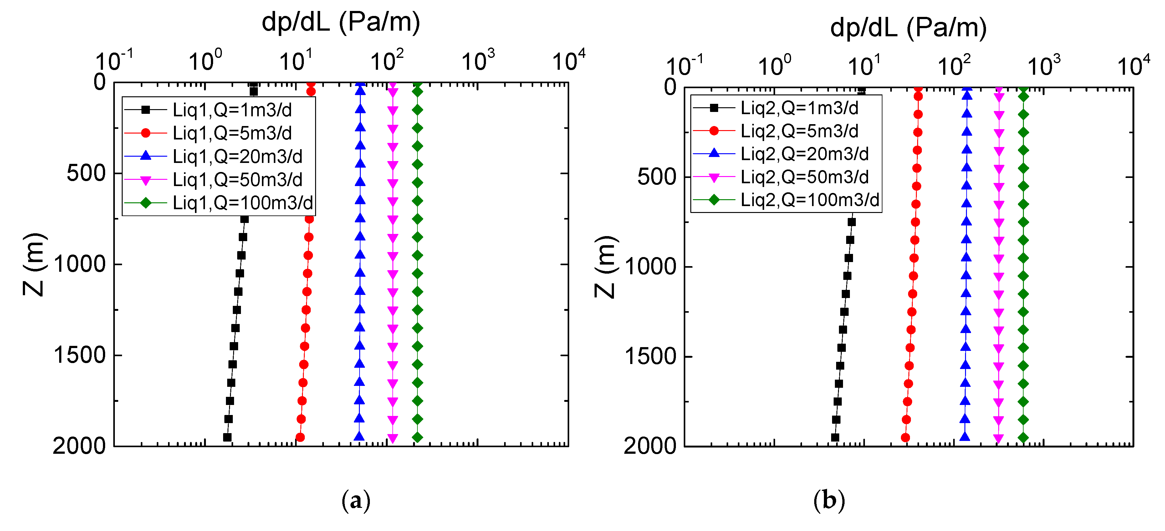
4.4. Hydraulic Pressure Drop in the Wellbore

The hydraulic pressure drop for liquids 1 and 2 is also influenced by injection rates. Figure 10 shows the influence of injection rates on the hydraulic pressure drop for liquids 1 and 2 at the total injection time (t = 7 days). The hydraulic pressure drop per unit meter for both liquid types increases by approximately two orders of magnitude as the injection rates increase from 1 m³/d to 100 m³/d. In general, the hydraulic pressure drop in the annulus (liquid 2) is higher than that in the tubing (liquid 1) at this parameter combination. Although increasing the injection rate can decrease the viscosity loss for the injected liquid, the hydraulic energy loss greatly increases.

4.5. Flowing Behavior and Hydraulic Friction in the Wellbore

Figure 11 shows the influence of injection rates on the Reynolds number and coefficient of friction at the total injection time (t = 7 days). The Reynolds number for both liquid types increases as injection rates increase from 1 m³/d to 100 m³/d. However, $\mathrm{Re}<<2000$. Specifically, the flow pattern for both liquid types is laminar flow. The Reynolds number of liquid 1 in inner tubing is approximately 3 times higher than that of liquid 2 in annular space. The coefficient of friction is defined as the reciprocal of the Reynolds number. In particular, Re increases, and the coefficient of friction decreases as the flowing rates increase. Although the expression for the coefficient of friction in the tubing and annulus is different (Equations 26 and 30), the tendency for both liquid types is similar. The coefficient of friction decreases by approximately two orders of magnitude as the injection rates increase from 1 m³/d to 100 m³/d.

5. Conclusions

Considering separate injection through the concentric dual-tubing, this study focuses on the polymer flowing characteristics during the injection process in the wellbore. A temperature–viscosity coupling model for the multilayer separate polymer injection process is derived. An estimate-correct method for the heat transfer process is then introduced to derive the numerical solution of this model. Lastly, the axial temperature distribution, viscosity distribution, hydraulic pressure drop, and flow pattern during the injection process is investigated. Based on the results, the viscosity of polymer solution can be obtained at the bottom hole of well which is useful for the polymer flooding calculation in the formation. Results are listed as follows:

(1) The temperature distribution of polymer solution is greatly influenced by the injection rate and injection time. At low injection rates, the temperature difference between polymer and formation is quite small. Formation temperature is the primary factor to influence the temperature of polymer solution. At high injection rates, commonly larger than 20 m³/d, the temperature increase of injected polymer is slight, commonly less than 5 °C under the given parameter combination.

(2) The viscosity of polymer solution is also greatly influenced by the injection rate and injection time, because the viscosity of polymer is affected by both shear and temperature. Under different flow rates, the polymer viscosity varies greatly and widely. Meanwhile, at low injection rates, commonly smaller than 20 m³/d, the axial viscosity distribution is greatly affected by formation temperature and the polymer viscosity at the bottom hole is obviously smaller than that at well head. However, at high injection rates, the influence from formation temperature is slight, polymer viscosity decrease is just about 2–3 vmPa·s.

(3) The hydraulic pressure drop is also greatly influenced by the injection rate. When the injection rate increases from 1 m³/d to 100 m³/d, the hydraulic pressure drop increases by approximately two orders of magnitude. Meanwhile, the coefficient of friction decreases by approximately two orders of magnitudes for the injected polymers in the tubing and annulus.

(4) The derived numerical model is meaningful and helpful for viscosity and energy loss estimation in the injection process. The model can give the axial distribution of polymer temperature, viscosity, and pressure drop under different injection rates and time. These parameters are meaningful for the polymer injection process in oilfields.

References

1. Garmeh, G.; Izadi, M.; Salehi, M.; Romero, J.L.; Thomas, C.; Manrique, E.J. Thermally active polymer to improve sweep efficiency of waterfloods: Simulation and pilot design approaches. SPE-144234-PA 2012, 15, 86–97. [Google Scholar] [CrossRef]
2. Al-Shakry, B.; Skauge, T.; Shaker Shiran, B.; Skauge, A. Polymer injectivity: Investigation of mechanical degradation of enhanced oil recovery polymers using in-situ rheology. Energies 2019, 12, 49. [Google Scholar] [CrossRef] [Green Version]
3. Sheng, J.J.; Leonhardt, B.; Azri, N. Status of polymer-flooding technology. J. Can. Pet. Technol. 2015, 54, 116–126. [Google Scholar] [CrossRef]
4. Wang, D.; Dong, H.; Lv, C.; Fu, X.; Nie, J. Review of practical experience by polymer flooding at Daqing. SPE Reserv. Eval. Eng. 2009, 12, 470–476. [Google Scholar] [CrossRef]
5. Gao, C. Viscosity of partially hydrolyzed polyacrylamide under shearing and heat. J. Pet. Explor. Prod. Technol. 2013, 3, 203–206. [Google Scholar] [CrossRef] [Green Version]
6. Godwin Uranta, K.; Rezaei-Gomari, S.; Russell, P.; Hamad, F. Studying the effectiveness of polyacrylamide (pam) application in hydrocarbon reservoirs at different operational conditions. Energies 2018, 11, 2201. [Google Scholar] [CrossRef] [Green Version]
7. Li, X.E.; Xu, Z.; Yin, H.; Feng, Y.; Quan, H. Comparative studies on enhanced oil recovery: Thermoviscosifying polymer versus polyacrylamide. Energy Fuels 2017, 31, 2479–2487. [Google Scholar] [CrossRef]
8. Sheng, J.J. Critical review of alkaline-polymer flooding. J. Pet. Explor. Prod. Technol. 2017, 7, 147–153. [Google Scholar] [CrossRef]
9. Olajire, A.A. Review of ASP EOR (alkaline surfactant polymer enhanced oil recovery) technology in the petroleum industry: Prospects and challenges. Energy 2014, 77, 963–982. [Google Scholar] [CrossRef]
10. Liao, G.; Wang, Q.; Wang, H.; Liu, W.; Wang, Z. Chemical flooding development status and prospect. Acta Pet. Sin. 2017, 38, 196–207. [Google Scholar]
11. Liang, S.; Liu, Y.; Hu, S.; Shen, A.; Yu, Q.; Yan, H.; Bai, M. Experimental study on the physical performance and flow behavior of decorated polyacrylamide for Enhanced Oil Recovery. Energies 2019, 12, 562. [Google Scholar] [CrossRef] [Green Version]
12. Sun, C.; Hou, J.; Pan, G.; Xia, Z. Optimized polymer enhanced foam flooding for ordinary heavy oil reservoir after cross-linked polymer flooding. J. Pet. Explor. Prod. Technol. 2016, 6, 777–785. [Google Scholar] [CrossRef] [PubMed]
13. Saboorian-Jooybari, H.; Dejam, M.; Chen, Z. Half-century of heavy oil polymer flooding from laboratory core floods to pilot tests and field applications. In Proceedings of the SPE Canada heavy oil technical conference, Calgary, AB, Canada, 9–11 June 2015. [Google Scholar]
14. Saboorian-Jooybari, H.; Dejam, M.; Chen, Z. Heavy oil polymer flooding from laboratory core floods to pilot tests and field applications: Half-century studies. J. Pet. Sci. Eng. 2016, 142, 85–100. [Google Scholar] [CrossRef]
15. Delamaide, E. Polymer flooding of heavy oil-from screening to full-field extension. In Proceedings of the SPE Heavy and Extra Heavy Oil Conference: Latin America, Medellin, Colombia, 24–26 September 2014. [Google Scholar]
16. Kuiqian, M.; Yanlai, L.; Lilei, W.; Xiaolin, Z. Practice of the early stage polymer flooding on LD offshore oilfield in Bohai bay of China. In Proceedings of the SPE Asia Pacific Enhanced Oil Recovery Conference, Kula Lumpur, Malaysia, 11–13 August 2015. [Google Scholar]
17. Sun, L.; Li, B.; Jiang, H.; Li, Y.; Jiao, Y. An injectivity evaluation model of polymer flooding in offshore multilayer reservoir. Energies 2019, 12, 1444. [Google Scholar] [CrossRef] [Green Version]
18. Tie, L.; Yu, M.; Li, X.; Liu, W.; Zhang, B.; Chang, Z.; Zheng, Y. Research on polymer solution rheology in polymer flooding for Qikou reservoirs in a Bohai Bay oilfield. J. Pet. Explor. Prod. Technol. 2019, 9, 703–715. [Google Scholar] [CrossRef] [Green Version]
19. Zheng, W.; Jiang, H.; Zhang, X.; Li, J.; Chen, M.; Ma, J. Offshore polymer flooding optimization using surrogate-based methodology. Pet. Sci. Technol. 2011, 29, 1227–1235. [Google Scholar] [CrossRef]
20. He, H.; Chen, Y.; Yu, Q.; Wen, X.; Liu, H. Optimization design of injection strategy for surfactant-polymer flooding process in heterogeneous reservoir under low oil prices. Energies 2019, 12, 3789. [Google Scholar] [CrossRef] [Green Version]
21. Liu, S.; Shen, A.; Qiu, F.; Liang, S.; Wang, F. Matching relationship and alternating injection for polymer flooding in heterogeneous formations: A laboratory case study of daqing oilfield. Energies 2017, 10, 1018. [Google Scholar] [CrossRef] [Green Version]
22. Sidiq, H.; Abdulsalam, V.; Nabaz, Z. Reservoir simulation study of enhanced oil recovery by sequential polymer flooding method. Adv. Geo-Energy Res. 2019, 3, 115–121. [Google Scholar] [CrossRef]
23. Wang, X.; Zhang, J.; Kang, X.; Wei, Z.; Meng, F.; Zhu, Y. Injection capacity analysis of downhole polymer injection pipe string in Bohai oilfield based on power law fluid model. China Offshore Oil Gas 2017, 29, 87–92. [Google Scholar]
24. Jennings, R.R.; Rogers, J.H.; West, T.J. Factors influencing mobility control by polymer solutions. SPE-2867-PA 1971, 23, 391–401. [Google Scholar] [CrossRef]
25. Weiss, W.W.; Baldwin, R.W. Planning and implementing a large-scale polymer flood. SPE-2867-PA 1985, 37, 720–730. [Google Scholar] [CrossRef]
26. Green, D.W.; Willhite, G.P. Enhanced Oil Recovery; Henry, L., Ed.; Doherty Memorial Fund of AIME, Society of Petroleum Engineers: Richardson, TX, USA, 1998; Volume 6. [Google Scholar]
27. Zhang, L.-J.; Yue, X.-A. Displacement of polymer solution on residual oil trapped in dead ends. J. Cent. South Univ. Technol. 2008, 15, 84–87. [Google Scholar] [CrossRef]
28. Zhang, Z.; Li, J.; Zhou, J. Microscopic roles of “viscoelasticity” in HPMA polymer flooding for EOR. Transp. Porous Media 2011, 86, 199–214. [Google Scholar] [CrossRef] [Green Version]
29. Restolho, J.; Serro, A.P.; Mata, J.L.; Saramago, B. Viscosity and surface tension of 1-ethanol-3-methylimidazolium tetrafluoroborate and 1-methyl-3-octylimidazolium tetrafluoroborate over a wide temperature range. J. Chem. Eng. Data 2009, 54, 950–955. [Google Scholar] [CrossRef]
30. Zheng, M.; Tian, J.; Mulero, Á. New correlations between viscosity and surface tension for saturated normal fluids. Fluid Phase Equilibria 2013, 360, 298–304. [Google Scholar] [CrossRef] [Green Version]
31. Haj-Kacem, R.B.; Ouerfelli, N.; Herráez, J.; Guettari, M.; Hamda, H.; Dallel, M. Contribution to modeling the viscosity Arrhenius-type equation for some solvents by statistical correlations analysis. Fluid Phase Equilibria 2014, 383, 11–20. [Google Scholar] [CrossRef]
32. Nian, Y.-L.; Cheng, W.-L. Evaluation of geothermal heating from abandoned oil wells. Energy 2018, 142, 592–607. [Google Scholar] [CrossRef]
33. Cheng, W.-L.; Huang, Y.-H.; Lu, D.-T.; Yin, H.-R. A novel analytical transient heat-conduction time function for heat transfer in steam injection wells considering the wellbore heat capacity. Energy 2011, 36, 4080–4088. [Google Scholar] [CrossRef]
34. Livescu, S.; Wang, X. Analytical downhole temperature model for coiled tubing operations. In Proceedings of the SPE/ICoTA Coiled Tubing and Well Intervention Conference and Exhibition, Woodlands, TX, USA, 25–26 March 2014. [Google Scholar]
35. Luo, L.; Tian, F.; Cai, J.; Hu, X. The convective heat transfer of branched structure. Int. J. Heat Mass Transf. 2018, 116, 813–816. [Google Scholar] [CrossRef]
36. Wooley, G.R. Computing downhole temperatures in circulation, injection, and production wells. SPE-2867-PA 1980, 32, 1,509–501,522. [Google Scholar] [CrossRef]
37. Smith, R.; Steffensen, R. Interpretation of temperature profiles in water-injection wells. SPE-2867-PA 1975, 27, 777–784. [Google Scholar] [CrossRef]
38. Okoya, S.S. Computational study of thermal influence in axial annular flow of a reactive third grade fluid with non-linear viscosity. Alex. Eng. J. 2019, 58, 401–411. [Google Scholar] [CrossRef]
39. Yi, L.-P.; Li, X.-G.; Yang, Z.-Z.; Sun, J. Coupled calculation model for transient temperature and pressure of carbon dioxide injection well. Int. J. Heat Mass Transf. 2018, 121, 680–690. [Google Scholar] [CrossRef]
40. Sun, F.; Yao, Y.; Li, X.; Yu, P.; Zhao, L.; Zhang, Y. A numerical approach for obtaining type curves of superheated multi-component thermal fluid flow in concentric dual-tubing wells. Int. J. Heat Mass Transf. 2017, 111, 41–53. [Google Scholar] [CrossRef]
41. Batra, R.L.; Sudarsan, V.R. Laminar flow heat transfer in the entrance region of concentric annuli for power law fluids. Comput. Methods Appl. Mech. Eng. 1992, 95, 1–16. [Google Scholar] [CrossRef]
42. Pinho, F.T.; Coelho, P.M. Fully-developed heat transfer in annuli for viscoelastic fluids with viscous dissipation. J. Non-Newton. Fluid Mech. 2006, 138, 7–21. [Google Scholar] [CrossRef]
43. Allanic, N.; Deterre, R.; Mousseau, P.; Couedel, D. Thermal Behavior of a Concentric Annular Polymer Flow. In AIP Conference Proceedings; AIP Publishing LLC: Kerala, India, 2019. [Google Scholar]
44. Li, Z.; Delshad, M. Development of an analytical injectivity model for non-newtonian polymer solutions. SPE J. 2014, 19, 381–389. [Google Scholar] [CrossRef]
45. Hasan, A.; Kabir, C. Heat transfer during two-phase flow in wellbores; Part I—formation temperature. In Proceedings of the SPE Annual Technical Conference and Exhibition, Dallas, TX, USA, 6–9 October 1991. [Google Scholar]
46. Holman, J.P. Heat Transfer, 10th ed.; McGraw-Hill: Dubuque, IA, USA, 2009. [Google Scholar]
47. Akter, S.; Hashmi, M.S.J. Analysis of polymer flow in a conical coating unit: A power law approach. Prog. Org. Coat. 1999, 37, 15–22. [Google Scholar] [CrossRef]
48. Monroy, F.; Hilles, H.M.; Ortega, F.; Rubio, R.G. Relaxation dynamics of langmuir polymer films: A power-law analysis. Phys. Rev. Lett. 2003, 91, 268302. [Google Scholar] [CrossRef]
Figure 1. Schematic diagram of allocator.
Energies 13 01637 g001
Figure 2. Schematic diagram of dual-tubing injection.
Energies 13 01637 g002
Figure 3. Schematic diagram for normal polymer injection well.
Energies 13 01637 g003
Figure 4. Schematic diagram for separate layer polymer injection well by concentric tubing.
Energies 13 01637 g004
Figure 5. The basic schematic of energy balance method and equivalent fluid domain. (a) is the volume and heat transfer in real dual-tubing system, (b) is the volume and heat transfer in simplified system.
Energies 13 01637 g005
Figure 6. Temperature distribution in downhole for different layers, as injecting rates increasing, the dynamic balance state becomes weak. The injecting rates are: (a) 1 m3/d, (b) 5 m3/d, (c) 20 m3/d, (d) 50 m3/d.
Energies 13 01637 g006
Figure 7. Temperature distribution in downhole for different layers. The influence of injecting time for inner layer is weaker than the outer layer. The injecting time are: (a) 1 d, (b) 5 d, (c) 10 d, (d) 20 d.
Energies 13 01637 g007
Figure 8. The influence of injecting rates on viscosity. As injecting rates increase, the viscosity loss greatly decreases. Normally, as the injecting rates are larger than 20 m3/d, the viscosity loss can be ignored.
Energies 13 01637 g008
Figure 9. The influence of injecting time on viscosity. As injecting time increasing, the viscosity at bottom slightly increases. Generally, the influence of injecting time is slight compared with injecting rates.
Energies 13 01637 g009
Figure 10. The injecting rates greatly influences the pressure drop.
Energies 13 01637 g010
Figure 11. The influence of injecting rates on Reynolds number and coefficient of friction. Generally, the injected polymers are laminar flow. (a) shows the relationship between injecting rates and Reynolds number. (b) shows the relationship between injecting rates and coefficient of friction.
Energies 13 01637 g011