Abstract
This paper proposes a new mass estimation for a vehicle system, utilizing the characteristics of engine torque local convex minimum, where the mass can be estimated based on the driving forces and the longitudinal accelerations only. Fundamentally, this approach generally requires no other information about an aerodynamic effect, a road grade, or a rolling friction, which is usually demanded by the existing well-known longitudinal dynamics and adaptive filter-based estimation methods. The effectiveness of the proposed approach was evaluated and validated by both TruckSim/Simulink co-simulation and actual field test data. It is found that the proposed estimation technique is more favorable for a situation where the vehicle is exposed to low-speed regions. In addition to this new mass estimation strategy, other new and current existing methods were explored and are reviewed here. Moreover, this study suggested a guideline for a hybrid-type mass estimation strategy to predict a mass by combining a new method with an existing one for every speed.
1. Introduction
It is very important to identify vehicle inertial parameters accurately in designing a vehicle control system. In most cases, the performance of an active safety system is, in general, guaranteed based on the assumption that the inertial parameters are already known or defaulted as unloaded conditions. However, this may not be applicable for a heavy truck undergoing unloaded and loaded up to almost double the Gross Vehicle Weight (GVW) frequently. In this regard, references [1,2] proposed the recursive least squares approach, forgetting for online estimation of vehicle mass and road grade. Here, we address that using multiple forgetting factors improves the transient and steady-state perspectives of estimation performance. Commonly, the existing mass estimation techniques rely on longitudinal dynamics, along with state estimation algorithms, such as the recursive least squares algorithm (RLS) [3] and Kalman filter (KF) [4]. Based on perturbation theory, Fathy [5] simplifies the mass estimation model with the differential equation of longitudinal dynamics. A robust parameter algorithm for the vehicle mass and driving resistance estimation has been proposed by [6], and it overcomes the drawbacks of outliers and insufficient excitation. To further improve the accuracy and robustness of the mass estimation, a torque observer was also applied into the system [7]. Moreover, in the literature [8,9,10,11,12,13], many have studied the method, simultaneously estimating the mass and road grade. Furthermore, reference [14] used an extended KF to estimate both mass and road grade. A Markov chain Monte Carlo method was applied to estimate vehicle inertial parameters [15]. The author of [16] presents a Global Positioning System (GPS) based vehicle mass and road grade estimation technique. Furthermore, reference [17] proposed more advanced estimation scheme with visual and acoustic data. Based on remotely collected video and audio data deducing a vehicle’s position, engine torque-induced frame twist, and engine speed, the vehicle’s mass-to-spring constant ratio can be calculated so that the vehicle mass can be obtained. Furthermore, reference [18] analyzed the system error of vehicle longitudinal dynamics in RLS estimation approach and addressed that, if the error is considered in an estimate, the estimation error can be reduced. However, most of the current mass estimation techniques require the parameters of longitudinal dynamics, such as aerodynamic parameters, rolling resistance coefficient, and so on, which are quite cumbersome to be measured accurately and possibly determined with some errors. The usage of such inaccurate parameters in the longitudinal dynamics consequently causes the significant estimation errors. In this regard, this study presents a new mass estimation approach based on a longitudinal dynamic model with the minimum system parameters. Specifically, this new mass estimation method utilizes the characteristics of vehicle behavior subject to engine torque local convex minimum, where the mass can be estimated based on driving force (i.e., a pure torque (force) delivered by an Engine to driving wheel) and longitudinal acceleration only, thereby, demanding no other information about an aerodynamic force, a road grade, or a rolling friction. This paper is organized as follows. Section 2 presents a new vehicle mass estimation strategy based on an engine torque local convex minimum characteristic. Section 3, Section 4 and Section 5 explore other new estimation methods and review the existing ones. The conclusion subsequently follows in Section 6.
2. Vehicle Mass Estimation Using the Characteristics of Engine Torque
This section proposes a new mass estimation for a vehicle system, utilizing the characteristics of engine torque local convex minimum, where the mass estimation can be possibly performed based on the driving force and the longitudinal acceleration only, without any other information about the forces acting on a vehicle system.
According to the forces shown in Figure 1, the longitudinal dynamics of a vehicle is given by the following equations:
where , , , and are a driving force, an aerodynamic force, a force due to road grade, and a rolling resistance, respectively; m is the vehicle mass. Other variables, , , , , and , are an engine torque, a final gear ratio, a transmission gear ratio, the efficiency of power train, and the effective radius of tire, respectively. The parameters , , , , , and are the air density, a drag coefficient, a frontal projected area, a longitudinal velocity, a road grade, and rolling friction coefficient.
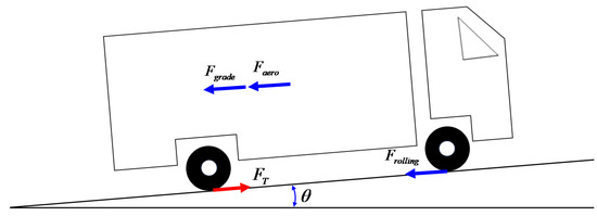
Figure 1.
Effective forces in longitudinal vehicle dynamics.
The total gear ratio is also obtained by the following equation:
where C and n are a constant and an engine rotational speed. It is a benefit for us to use Equation (2) since it requires no information about a gear shift status, as long as v and n are available.
Next, let’s consider the longitudinal vehicle dynamics for the two consecutive times, denoted by t and t − 1:
If we assume that the road grade and friction are not varied from the previous time, t − 1 to the current one t, the conditions and are possibly feasible.
Together with the above conditions, subtracting Equation (4) from Equation (5) yields the following:
Moreover, for the low-speed regions, the effect of aerodynamic forces (the last terms in Equation (6)) is relatively small, and the condition can especially be made near the local convex minimum of engine torque. This point of view is discussed in the Appendix A.
Consequently, incorporating into Equation (6) becomes Equation (7):
Equation (7) indicates that the mass estimation can be achieved without identifying any data and information related to other forces, , , and , when the vehicle experiences the local convex minimum of engine torque in the low speed regions. This means that this mass estimation strategy proposed here is relatively convenient and compact compared to other existing approaches usually relied on the fully expressed longitudinal dynamics, Equation (1).
2.1. Extraction of Multiple Local Convex Region from Engine Torque Data
To achieve the mass estimation based on Equation (7), it is crucial to detect the minimums in the local convex regions of engine torque, , available via Controller Area Network (CAN). Therefore, this section presents the simple detection algorithm for the convex minimum of the given data. The following three circular buffers accepting the five consecutive engine torques (), the driving forces (), and the longitudinal accelerations () were employed for further design.
Figure 2 illustrates how the data of each buffer are managed. Specifically, when new data are conveyed to each circular buffer, the data corresponding to the first index in each buffer are removed, the remaining data (i.e., 2nd through 5th data) fill the first four array of each buffer in the sequential order, and the newly arrived data then occupy the last array of each buffer. This procedure is continuously repeated, as long as the estimation process is active.
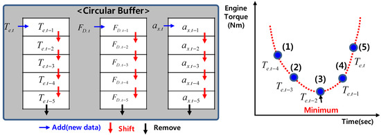
Figure 2.
Circular buffers for data management and the minimum in local convex region of engine torque.
Next, from the data stored into circular buffer, the minimum value of convex region for can be found according to Equation (11). At the moment when Equation (11) is satisfied, the corresponding driving force and the longitudinal acceleration data stored in the 2nd and 3rd array of circular buffer will be the candidate data for a further process and distinguished from others by adding an upper-subscript asterisk (as shown in Equation (12)):
In other words, the data in Equation (12) that correspond to the prior moment right before the minimum in convex region (i.e., ) and the one to be captured as the minimum (i.e., ), will be submitted to next step of vehicle mass estimation.
The entire mass estimation process is described in Figure 3, and it can be seen from the given flow that the data management, the convex minimum detection, and the Kalman estimation are processed in sequential order. The details of the Kalman estimation are presented in the next section.
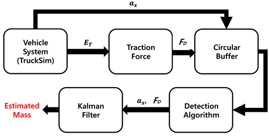
Figure 3.
Entire data flow for estimation.
2.2. Kalman-Filter-Based Mass Estimation
The data captured by the detection algorithm in Section 2.1 are now available for the mass estimation. However, before feeding such data to the Kalman filter, the fidelity and quality of the selected sensor data must be examined.
Although the estimation via an adaptive filter is capable of managing the abnormality of sensor data to some extent, it is essential that the infidelity data should be least involved, to guarantee an accurate estimation performance.
To meet such a need, the following conditions should be enforced:
where , , , , , and are constant thresholds quantified based on simulation results and actual field test data. Specifically, while Equation (13) indicates the minimum and maximum boundary of driving forces and accelerations, Equation (14) is used to prevent the involvement of radically changed two consecutive datasets jumping into the estimation.
In addition, since the estimation approach is fundamentally derived based on pure longitudinal vehicle dynamic model, the following conditions are also required, in order to maintain the validity of longitudinal dynamics,
where , , , , and are the steering-wheel angle, brake master cylinder pressure, lateral acceleration, yaw rate, and each wheel slip ratio, which can be obtained by ABS/ESP. As done before, , , , , and are constant thresholds determined based on simulation results and actual field test data. The conditions in Equation (15) indicate non-excessive steering, non-braking, small lateral, and yaw motions of the vehicle body, as well as insignificant wheel slips.
Considering the conditions of Equations (14) and (15), the trusted data is redefined with an additional subscript, K, to each variable, as follows:
Finally, the data in Equation (16) is used in the actual estimation via the Kalman filter.
Next, let’s consider the following prediction dynamics based on Equation (7):
where the subscripts k − 1/k − 1 and k/k − 1 indicate the prior state and the current predicted one. Moreover, is obtained by Equation (16).
Defining the predicted state vector of the Kalman filter as and the previous one as , and rearranging (17) for the 1st order form, gets the following:
Consequently, the predicted error covariance and the innovation in update stage are given by the following equations:
where is the covariance of process noise. Moreover, and are obtained by (16).
The optimal Kalman gain is now provided by the following:
The updated state and covariance estimates are obtained by the following:
Finally, based on the datasets detected by Equation (11) and filtered by Equation (13) through Equation (15), the mass estimation can be accomplished via Equation (18) through Equation (24).
2.3. Simulation and Actual Test-Data-Based Estimation Results
In this section, based on TruckSim/Simulink and actual field test data, the estimation performances are discussed, to investigate the effectiveness of the proposed mass estimation strategy. The target truck selected was the H-Mega Truck, shown in Figure 4; it can load up to approximately 5 tons (medium-duty).
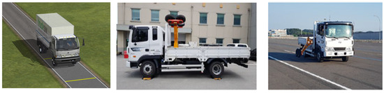
Figure 4.
TruckSim model and actual vehicle for H-Mega Truck.
Before proceeding, to investigate the validity of Equation (7), in Figure 5, we presented the absolute difference between two consecutive longitudinal velocities, , based on actual test data. The red circles in Figure 5 represent the detected point via Equation (11), which is at the local convex minimums of an engine torque. Compared to other , the value of detected point is relatively small, which is usually less than 0.02 km/h, resulting in the assumption for Equation (7) is possibly doable near the local convex minimums of an engine torque.
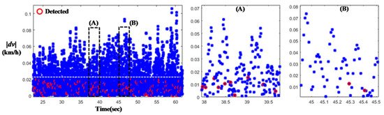
Figure 5.
Absolute differences of longitudinal velocity.
Figure 6 presents the estimates for four different cases, 5420, 6420, 7420, and 8420 kg, using TruckSim/Simulink co-simulation. Figure 6a represents the scenario of longitudinal velocities for four situations, and Figure 6b indicates the estimates for the given vehicle masses. The dotted lines in Figure 6b are the true mass of vehicle for each case. Here, it should be mentioned that the initial state of the Kalman filter (i.e., at a time t = 0) is randomly assigned. It is observed from Figure 6b that the estimates well agree with true ones and the estimation actively occurs below 18 km/h, which is the low-speed region. In addition, the estimation strategy utilizes the moment satisfying Equation (7); thus, it is valuable to explore the performance for the different data handling sampling times. Figure 7 shows the estimation performances based on several sampling frequencies (1000, 200, 100, and 50 Hz). According to the results, the 1000 or 50 Hz sampling frequency slightly degrades the estimation performance, while 100 Hz guarantees the estimation performance with some error. Therefore, the suitable sampling frequency is 200 Hz; thus it has been used in an actual vehicle field test.
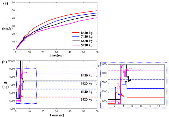
Figure 6.
Mass estimation results (TruckSim): (a) Vehicle Speeds; (b) Mass estimates.
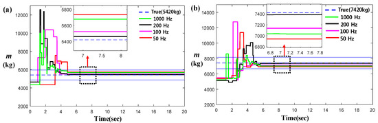
Figure 7.
Estimation performances, based on the data sampling frequencies 1000, 200, 100, and 50 Hz (TruckSim). (a) Mass estimates for 5420 kg; (b) Mass estimates for 7420 kg.
Figure 8 shows the estimates for three different road grades; 0 deg. (i.e., flat), 3 deg. and 6 deg. Figure 8a,b indicates the results of the case m = 6420 kg, while Figure 8c,d represents the outcomes for the case m = 7420 kg. Due to the characteristic of a given estimation approach, it should predict the given actual masses, regardless of road grades. According to Figure 8, we can see that the estimates capture the given actual mass for three different cases. Hence, compared to estimation mechanisms in other existing approaches [1,2,3,4,5,6,7,8,9,10,11,12,13,14,15], it is of tremendous benefit to predict the unknown mass, without perceiving the information of a road grade.
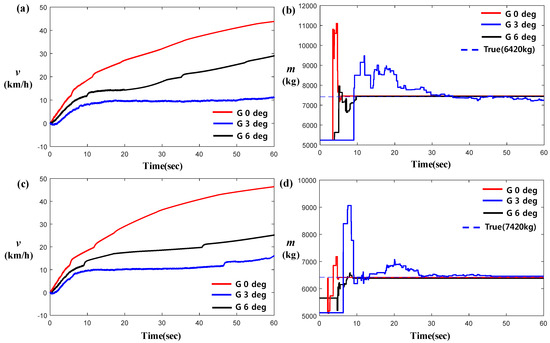
Figure 8.
Estimation performances for three different road grades based on TruckSim simulation (6420 kg for (a,b); and 7420 kg for (c,d)).
Furthermore, Figure 9 shows the estimation results of unloaded truck based on two different actual field test datasets. Figure 9a,c,e indicates the case that the vehicle has been accelerated from 0 to 90 km/h, within 30 s, while Figure 9b,d,f describes the situation where it is exposed to the low speeds (i.e., from 0 to 30 km/h, for 100 s). Figure 9c,d shows the detection performance for the local convex minimum of engine torque. Here, the circle dots indicate the detected ones (i.e., satisfying Equation (11) only), and the circle-asterisk dots are detected and actually used for the Kalman estimation (i.e., defined in Equation (16)). As shown in Figure 9e,f, it is found that the errors between estimates and true ones are respectively 134 and 30 kg. As shown in the results in Figure 6, Figure 7 and Figure 8, the proposed estimation strategy mostly takes advantages from the data belonging to the range of low speeds; thus, the driving scenario shown in Figure 9a hardly produces suitable data to secure a desired performance. In other words, a particular driving situation may not generate sufficient favorable raw data for the successful estimation. However, since the case in Figure 9b particularly contains more favorable situation (i.e., low speeds) for an estimation process, the error becomes insignificant. Furthermore, Figure 10 describes the estimation results of a fully loaded truck for two different driving scenarios. Estimates tend to be very similar to those obtained from unloaded trucks. It is apparently exhibited from Figure 9 and Figure 10 that a more accurate estimation can be guaranteed if the data in low-speed regions are presented in the estimation process. Here, we proposed a new mass estimation method and evaluated its effectiveness. According to the results presented here, it is found that the performance of the given estimation approach is beneficial for the situation where the vehicle is exposed to the low-speed region and degraded otherwise.
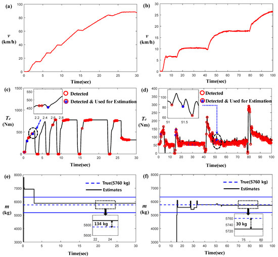
Figure 9.
Mass estimation results for two different scenarios based on actual filed test data (unloaded/5760 kg), (a,b) Vehicle Speeds, (c,d) Engine Torques, (e,f) Mass estimates.
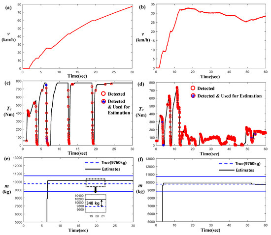
Figure 10.
Mass estimation results for two different scenarios based on actual filed test data (fully loaded/9760 kg), (a,b) Vehicle Speeds, (c,d) Engine Torques, (e,f) Mass estimates.
3. Vehicle Longitudinal Velocity Based Mass Estimation
In addition to the new approach discussed in Section 2, this section describes how to estimate vehicle mass based on the longitudinal vehicle velocity and EKF (Extended Kalman Filter). This approach can be used under the circumstances where the acceleration of the vehicle is not available for mass estimation. Here, we do not consider the effect of road grade. Therefore, under the assumption that the vehicle is driven on the “zero” grade road, discretizing Equation (1) with a sampling time, , yields the following:
where k − 1 and k are the previous time step and the current one.
Rearranging Equation (25) produces the following:
where .
Based on Equation (26), the prediction model for both the velocity and the mass can be derived as follows:
Defining estimate state vector as and using the Jacobian for the set of nonlinear system Equations (27) and (28), the error covariance is as follows:
where and .
The rest of the procedure for the update is given by the following equations:
where .
The performance of the velocity-based mass estimation approach was evaluated through TruckSim simulation and actual test data, and the results are presented here. Figure 11 includes the estimated results for four different situations: 5420, 6420, 7420, and 8420 kg. It is found that the estimates mutually agree with the actual mass at speeds above 30 km/h, and the deviation between the estimates and the actual ones with large overshoots can be obviously recognized below 30 km/h. Furthermore, Figure 12 and Figure 13 show the estimates for actual test data. As predicted by the simulation results in Figure 11, under the driving scenario where the velocity is below 30 km/h, the estimates never reach the true ones (see Figure 12a and Figure 13a). However, the outcomes in Figure 12b and Figure 13b exhibit the desired estimation performances for the circumstance involving high speeds. It is clear that the performance of this approach is quite opposed to the trend captured by new approach presented in Section 2.
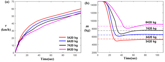
Figure 11.
Mass estimation results of Velocity-based approach based on TruckSim simulation. (a) Vehicle Speeds; (b) Mass estimates.
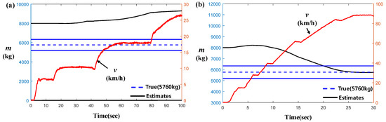
Figure 12.
Mass estimation results of V-based approach for two different scenarios based on actual filed test data (5760 kg). (a) Mass estimate in low speeds; (b) Mass estimate in high speeds.
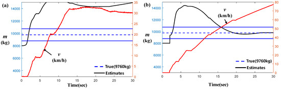
Figure 13.
Mass estimation results of V-based approach for two different scenarios based on actual filed test data (9760 kg). (a) Mass estimate in low speeds; (b) Mass estimate in high speeds.
4. Predefined-Particle-Mass-Based Mass Estimation
This study also discusses the “rigorous and brutal (Monte Carlo)” method to use the predefined mass particles for predicting vehicle mass. Sometimes, the estimation performance of an adaptive filter, such as the Kalman filter or RLS, is not reliable or robust for the particular cases. However, the ‘Monte Carlo’ style copes well with the complicate estimation problem, although the computational load is quite consumed. Hence, we have applied this approach to mass estimation in very elementary but powerful manner.
Again, neglecting , Equation (1) becomes the following:
where .
Creating the set of assumed particles for mass, we get the following:
where , , and are, respectively, the particle mass, base-line mass, and an incremental mass. Moreover, N is the total number of particles.
Based on the particle masses in Equation (36), the corresponding set of acceleration can be generated by Equation (35):
By comparing the sets of acceleration in Equation (37) with the actual acceleration obtained via a sensor, the most minimum of m can be found for every time step, such that we obtain the following:
where is the index for the minimum among () for the k-th time step.
For each time step, the estimates of mass are recursively updated by Equation (40):
where is a particle mass corresponding to the index in Equation (39). The derivation of Equation (40) is given in the Appendix A.
It should be noted that the computational load of this approach is burdensome, as the number of particles, , increases. However, it should be mentioned that the accuracy of estimation can be improved by employing a larger number of particles.
The performance of the particle-mass-based estimation approach was discussed here. Figure 14 includes the estimated results for four different cases: 5420, 6420, 7420, and 8420 kg. It is clear that the estimates mutually agree with the actual ones right above 20 km/h. Furthermore, Figure 15 and Figure 16 show the estimates for both actual tests, unloaded and fully loaded cases. Although we observe the transient responses, such as peaks and deviations in the low-speed regions from both cases in Figure 15 and Figure 16, the estimates arrive near the true ones in the range of high speed.
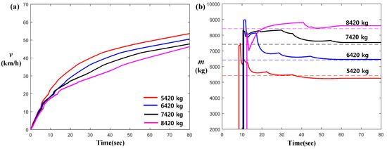
Figure 14.
Mass estimation results of particle mass (PM)-based approach (50 particles used/TruckSim). (a) Vehicle Speeds; (b) Mass estimates.
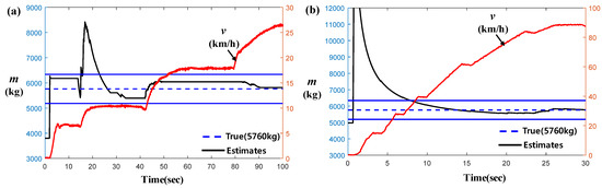
Figure 15.
Mass estimation results of PM-based approach for actual filed test data (5760 kg). (a) Mass estimates in low speeds; (b) Mass estimates in high speeds.
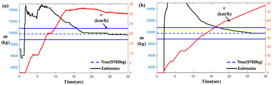
Figure 16.
Mass estimation results of PM-based approach for actual filed test data (9760 kg). (a) Mass estimates in low speeds; (b) Mass estimates in high speeds.
5. Recursive Least Square Based Mass Estimation
This section reviews the well-known mass estimation approach, RLS (Recursive Least Square), and evaluates its performance based on the simulation and actual test.
Disregarding the road grade, according to Equation (1),
where .
The linear regression model for predicting at the k-th time step is followed by Equation (42):
where is a regressor obtained by a sensor (here, is assumed to be known), and is an unknown parameter to be estimated.
The estimates for the unknown are recursively updated by Equation (43):
where is a positive forgetting factor, ranging from 0 to 1, and which is available via CAN data.
The performance of the RLS-based mass estimation approach was explored here. Figure 17 shows the estimates for 5420, 6420, 7420, and 8420 kg. It is apparently shown that the estimates accomplish the mutual agreement with the true ones at above 20–30 km/h. Moreover, Figure 18 and Figure 19 describe the estimates for given actual test data. Like the tendencies of both V-based and PM-based approaches discussed in the Section 3 through Section 4, predicting the true mass in high speed, the RLS-based approach presented here shows its excellence in the high-speed region.
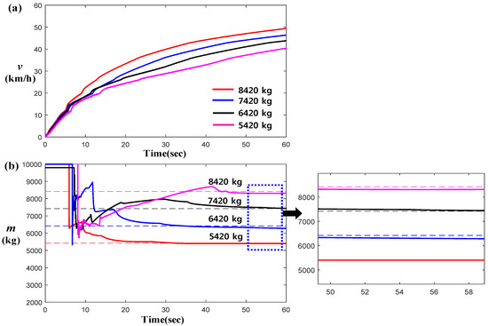
Figure 17.
Mass estimates results via TruckSim. (a) Vehicle Speeds; (b) Mass estimates.

Figure 18.
Mass estimates results for two different scenarios (actual filed test data/5760 kg). (a) Mass estimates in low speeds; (b) Mass estimates in high speeds.
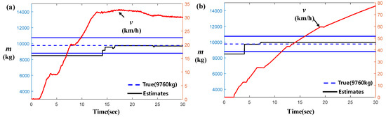
Figure 19.
Mass estimates results for two different scenarios (actual filed test data/9760 kg). (a) Mass estimates in low speeds; (b) Mass estimates in high speeds.
6. Conclusions
This study primary focuses on a new vehicle mass estimation that utilizes the characteristics of engine torque local convex minimum (where the mass can be estimated based on driving forces and longitudinal accelerations only) and deals with other various mass estimation approaches. The new approach proposed here has the great advantage of estimating vehicle mass without perceiving other effective resistance forces in the aspect of a pure longitudinal dynamics. In addition, based on both simulations and actual field tests, it is found that the new method is suitable to predict the vehicle mass for the situation in which the vehicle is exposed to low speeds. On the other hand, other approaches (V-based/PM-based/RLS based) demonstrated a better estimation performance when it was involved with intermediate- and high-speed regions. Therefore, we can suggest that combining the new one with V-based, PM-based, or RLS-based approaches possibly yields an excellent estimation strategy to cope with all possible ranges of vehicle speed. This hybrid concept is briefly outlined here and specified in Figure 20, which logically synthesizes two individually estimated masses according to the ranges of longitudinal velocity (this will be our next research). Additionally, the simple synthesis of two individual mass estimates (calculated by ) was illustrated in Figure 21b, based on two separate estimates (shown in Figure 21a), using a synthesis weight function in Figure 22. Merging the two distinct estimates via the synthesis weight function, we can obtain the better estimates in the entire range of vehicle speeds by eliminating the transient part of low-speed regions. This concept will be thoroughly investigated in our next research study. Finally, it is hoped that this work can provide insight for one who is majorly concerned with achieving an accurate mass estimation for a heavy truck, especially for low speed.
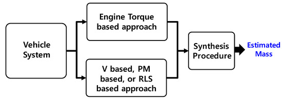
Figure 20.
Hybrid mass estimation strategy.
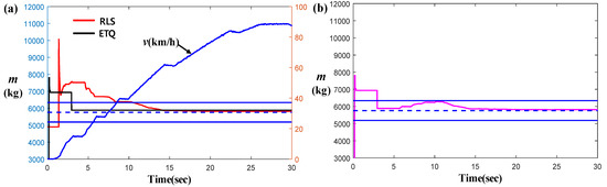
Figure 21.
Synthesized masse based on synthesis weight function in Figure 22 (RLS: recursive-least-square-based estimate, and ETQ: engine-torque-based result). (a) Two individual mass estimates; (b) Combined mass estimates via synthesis weight function.
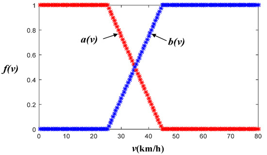
Figure 22.
Synthesis weight function (weight vs. velocity).
Author Contributions
Conceptualization, G.C. and D.J.; methodology, D.J. and G.C.; software, D.J. and G.C.; validation, D.J.; formal analysis, D.J.; investigation, D.J.; writing—original draft preparation, D.J. and G.C.; writing—review and editing, D.J. and G.C.; visualization, D.J.; supervision, G.C.; project administration, G.C.; funding acquisition, G.C. All authors have read and agreed to the published version of the manuscript.
Funding
This research received the funding from the KETEP, Resources Development Programs (Grant No. 20194010201800).
Acknowledgments
This work was supported by the KETEP, as Human Resources Development Programs (Grant No. 20194010201800). Also, this study was developed by the Ministry of Commerce, Industry and Energy “Development of pneumatic automatic emergency braking system for medium and large commercial vehicles over 4.5 tons”, task number: 20002814.
Conflicts of Interest
The authors declare no conflict of interest.
Appendix A
The condition can be made near the local convex minimum of engine torque.
Revisiting Equation (4), we can see the following:
Specifically,
Assuming that the road grade is close to 0 deg. (i.e., = 0), (A2) becomes the following:
Considering the absolute ratio of Equation (A3) for two consecutive times, t − 1 and t are given by the following equation:
Here, the subscript t − 1 is the prior moment right before the minimum of convex region, and t is the time to capture the minimum of convex region, as shown in Figure A1.
At the low-speed regions, the aerodynamic forces and in Equation (A4) are insignificant to other forces. Therefore, we get the following:
Since the driving force (i.e., ) is proportional to an engine torque, , the last part of Equation (A5) meets the following inequality:

Figure A1.
A typical local convex minimum in an engine torque.
Figure A1.
A typical local convex minimum in an engine torque.

On other hand, the accelerations of vehicle at the time steps t − 1 and t are approximated by the following:
The absolute ratio of two entities in (A7) yields is calculated as follows:
Finally, by combining Equation (A8) with Equation (A6), we can conclude the following:
Equation (A9) implies that the velocity difference at the local convex minimum region is relatively smaller than other . Therefore, it is possible that for the time steps, t − 1 and t, in the local convex.
Moreover, the derivation of (40) is presented here. Considering the average of mass for k − 1th and kth time step, we get the following:
Subtracting one from another yields the following:
Consequently,
References
- Vahidi, A.; Druzhinina, M.; Stefanopoulou, A.; Peng, H. Simultaneous Mass and Time-Varying Grade Estimation for Heavy-Duty Vehicles. In Proceedings of the American Control Conference, Denver, CO, USA, 4–6 June 2003. [Google Scholar]
- Vahidi, A.; Stefanopoulou, A.; Peng, H. Recursive least squares with forgetting for online estimation of vehicle mass and road grade: Theory and experiments. Veh. Syst. Dyn. 2005, 43, 31–55. [Google Scholar] [CrossRef]
- Feng, Y.; Xiong, L.; Yu, Z.; Qu, T. Recursive least square vehicle mass estimation based on acceleration partition. Chin. J. Mech. Eng. 2014, 27, 448–459. [Google Scholar] [CrossRef]
- Eriksson, A. Implementation and Evaluation of a Mass Estimation Algorithm. Master’s Thesis, Kungliga Tekniska Högskolan, Stockholm, Sweden, 2009. [Google Scholar]
- Fathy, H.K.; Kang, D.; Stein, J.L. Online Vehicle Mass Estimation Using Recursive Least Squares and Supervisory Data Extraction. In Proceedings of the American Control Conference, Seattle, WA, USA, 11–13 June 2008. [Google Scholar]
- Altmannshofer, S.; Endisch, C. Robust Vehicle Mass and Driving Resistance Estimation. In Proceedings of the American Control Conference Boston Marriott Copley Place, Boston, MA, USA, 6–8 July 2016. [Google Scholar]
- Ghosh, J.; Foulard, S.; Fietzek, R. Vehicle Mass Estimation from CAN Data and Drivetrain Torque Observer; SAE Technical Paper 2017-01-1590; SAE: Warrendale, PA, USA, 2017. [Google Scholar]
- Mahyuddin, M.N.; Na, J.; Herrmann, G.; Ren, X.; Barber, P. Adaptive observer-based parameter estimation with application to road gradient and vehicle mass estimation. IEEE Trans. Ind. Electron. 2014, 61, 2851–2863. [Google Scholar] [CrossRef]
- Sun, Y.; Li, L.; Yan, B.; Yang, C.; Tang, G. A hybrid algorithm combining EKF and RLS in synchronous estimation of road grade and vehicle’ mass for a hybrid electric bus. Mech. Syst. Signal Process. 2016, 68–69, 416–430. [Google Scholar] [CrossRef]
- Kidambi, N.; Harne, R.L.; Fujii, Y.; Pietron, G.M.; Wang, K.W. Methods in Vehicle Mass and Road Grade Estimation. SAE Int. J. Passeng. Cars Mech. Syst. 2014, 7, 981–991. [Google Scholar] [CrossRef]
- Mcintyre, M.L.; Ghotikar, T.J.; Vahidi, A.; Song, X.; Dawson, D.M. A two-stage lyapunov-based estimator for estimation of vehicle mass and road grade. IEEE Trans. Veh. Technol. 2009, 58, 3177–3185. [Google Scholar] [CrossRef]
- Wang, Z.; Qin, Y.; Gu, L.; Dong, M. Vehicle System State Estimation Based on Adaptive Unscented Kalman Filtering Combing with Road Classification. IEEE Access 2017, 5, 27786–27799. [Google Scholar] [CrossRef]
- Kim, S.; Shin, K.; Yoo, C.; Huh, K. Development of algorithms for commercial vehicle mass and road grade estimation. Int. J. Automot. Technol. 2017, 18, 1077–1083. [Google Scholar] [CrossRef]
- Lei, Y.; Fu, Y.; Liu, K.; Zeng, H.; Zhang, Y. Vehicle mass and road grade estimation based on extended kalman filter. Trans. Chin. Soc. Agric. Mach. 2014, 45, 9–13. [Google Scholar]
- Miller, E.; Konan, A.; Duran, A. Bayesian Parameter Estimation for Heavy-Duty Vehicles; SAE Technical Paper 2017-01-0528; SAE: Warrendale, PA, USA, 2017. [Google Scholar] [CrossRef]
- Bae, H.S.; Ryu, J.; Gerdes, J.C. Road Grade and Vehicle Parameter Estimation for Longitudinal Control Using GPS. In Proceedings of the IEEE Conference on Intelligent Transportation Systems, Oakland, CA, USA, 25–29 August 2001. [Google Scholar]
- McKay, T.R.; Salvaggio, C.; Faulring, J.W.; Sweeney, G.D. Sweeney, Remotely detected vehicle mass from engine torque-induced frame twisting. Opt. Eng. 2017, 56, 063101. [Google Scholar] [CrossRef]
- Lin, N.; Zong, C.; Shi, S. The Method of Mass Estimation Considering System Error in Vehicle Longitudinal Dynamics. Energies 2019, 12, 52. [Google Scholar] [CrossRef]


© 2020 by the authors. Licensee MDPI, Basel, Switzerland. This article is an open access article distributed under the terms and conditions of the Creative Commons Attribution (CC BY) license (http://creativecommons.org/licenses/by/4.0/).