Abstract
The paper proposes the validation of the latest System Advisor Model (SAM) vs. the experimental data for concentrated solar power energy facilities. Both parabolic trough, and solar tower, are considered, with and without thermal energy storage. The 250 MW parabolic trough facilities of Genesis, Mojave, and Solana, and the 110 MW solar tower facility of Crescent Dunes, all in the United States South-West, are modeled. The computed monthly average capacity factors for the average weather year are compared with the experimental data measured since the start of the operation of the facilities. While much higher sampling frequencies are needed for proper validation, as monthly averaging dramatically filters out differences between experiments and simulations, computational results are relatively close to measured values for the parabolic trough, and very far from for solar tower systems. The thermal energy storage is also introducing additional inaccuracies. It is concluded that the code needs further development, especially for the solar field and receiver of the solar tower modules, and the thermal energy storage. Validation of models and sub-models vs. high-frequency data collected on existing facilities, for both energy production, power plant parameters, and weather conditions, is a necessary step before using the code for designing novel facilities.
1. Introduction
The System Advisor Model (SAM) code is free software [1], very popular among policymakers and engineers. SAM can model many renewable energy facilities, including concentrating solar power systems for electric power generation, parabolic trough, or solar towers. The software is also able to model industrial process heat from the parabolic trough. A more detailed description of SAM can be found in [2,3,4]. Concentrating solar power modeling details may also be found in [5,6,7]. This software has not been validated yet vs. the latest concentrated solar power energy facilities that recently started operation in the US, with real-world production data available, and a reasonable guess of the weather conditions available. This contribution addresses this significant research gap.
A concentrating solar power parabolic trough is much simpler and reliable than a concentrating solar power solar tower. They still deliver much better capacity factors ε (ratio of average generating power to nominal power) in the real world (experience of plants built and operated so far with information available) despite the theoretically inferior performances in the virtual reality of model computations [8,9,10,11,12]. With reference to wind and solar (photovoltaic), concentrating solar power has, if coupled to thermal energy storage, the advantage of dispatchability vs. intermittency and variability [13,14,15]. Hence, concentrating solar power with thermal energy storage has huge potential in a world characterized by significant renewable energy supply. While wind and solar photovoltaic are unable to supply any given output at a given time without external energy storage (the Australian National Electricity Market data tell us that even installed capacity of 18.1 GW sometimes is not enough to deliver 0.2 GW to the grid in cases, for example, of low wind after sunset), the coupling of concentrating solar power with molten salt thermal energy storage is extremely attractive, as it may produce fully dispatchable energy.
While the concentrating solar power solar tower coupled with thermal energy storage has so far performed badly in the real world, the concentrating solar power parabolic trough with thermal energy storage is already delivering good performances, [8,9,10,11,12], even if still less than the predictions. Solar photovoltaic works with annual average ε about 0.27–0.29, but with much larger than the capacity factor high-frequency standard deviations, for coefficients of variability in excess of unity [15]. While in the virtual reality of model computations concentrating solar power with thermal energy storage may achieve much larger and more uniform ε, with average ε well in excess of 0.5, also addressing the issues of lack of production during night times, and drastically reduced production with clouds, with dramatically reduced standard deviations, the best real-world experience has so far delivered an annual average ε of about 0.36 (Solana). By contrast with photovoltaic, concentrating solar power, especially the solar tower, suffers from cloud coverage, and this may considerably affect the accuracy of the models.
As concluded in [8,9,10,11,12], the concentrating solar power parabolic trough has the potential, once a satisfactory design will be industrialized, to deliver the same or better than photovoltaic costs of electricity without any thermal energy storage. Once intermittency and unpredictability are factored in the costs, the addition of thermal energy storage, similarly in need of a satisfactory design to be industrialized, will be then cost-effective with wind and solar photovoltaic requesting battery energy storage.
The condenser of concentrating solar power that frequently adopts low maximum temperature steam Rankine cycle is usually air cooling or evaporative cooling. In the operation of concentrating solar power, additional to the solar direct normal irradiance (DNI), temperature and humidity also affect the performance.
The major issue facing concentrating solar power is the over-optimistic claims that have not come true in the real world (see the Crescent Dunes plant working at annual ε of 0.15 down from the planned larger than 0.52 ε of the models), that may jeopardize the further expansion of technology otherwise of great potential.
The latest concentrating solar power parabolic trough and solar tower performance data permit us to determine the best design option to consider. Reference [16] includes 7 projects worldwide of net capacity >100 MW and that are operational. Only 4 of them have a net capacity >150 MW. With the additional requirement of easily accessible real-world production data, the number of facilities to consider above 100 MW capacity, operational, and with experimental data, reduces to 5. These 5 facilities are all in the US, the 377 MW Ivanpah (Ivanpah Solar Electric Generating SystemI, ISEGS), the 250 MW Solana, Genesis, and Mojave, and the 110 MW Crescent Dunes. ISEGS started production 01/2014, Solana 10/2013. Genesis 03/2014, Mojave 12/2014 and Crescent Dunes 11/2015. These facilities are very recent, and thus the state-of-the-art of the technologies. The specific technology is solar tower, no thermal energy storage, natural gas boost for ISEGS; parabolic trough, thermal energy storage of 6 hours, no natural gas boost, for Solana; parabolic trough, no thermal energy storage nor natural gas boost, for Genesis and Mojave; solar tower, thermal energy storage of 10 hours and no natural gas boost for Crescent Dunes.
The production data of ISEGS indicates ε in the low 20%, despite burning substantial amounts of natural gas, is everything but planned. This translates in larger generating costs as well as the emission of air pollutants and CO2. By accounting for the natural gas energy at the thermal efficiency of a combined cycle gas turbine plant, almost double the thermal efficiency of a solar cycle steam turbine plant, the corrected ε drastically reduces to less than 15%. The planned ε was 32.68%, with a much-limited boost by natural gas [8]. As this plant features a significant contribution by natural gas combustion, with a schedule unknown, ISEGS is not considered in the validation exercise.
Crescent Dunes had a planned ε of 51.89%. However, it is working at about 10% ε. The plant has been out of service many times [8]. This plant is included in the validation exercise, despite performing well below expectations. While the annual averages below expectations suffer from discontinued production, the monthly averages are an indication of the inaccuracy of the modeling approach.
Better performing is the parabolic trough technology. A parabolic trough is simpler and more reliable than a solar tower. Solana has a production more than 10% less than planned, but much better than Crescent Dunes, and better than ISEGS. While the planned ε was 43.11%, the latest ε is 36.40%. Genesis and Mojave, also featuring the more established parabolic trough technology without thermal energy storage, are performing about the design values, less than Solana. The actual ε is 28.11% for Genesis, exceeding the planned ε of 26.48%. Mojave is similarly performing above the design value but recently has dropped production to 24.6% vs. the planned 27.40%. Solana, Genesis, and Mojave are included in the validation exercise. The latest 12-months moving averages of the ε are Ivanpah* (with the superscript symbol * we indicate that the natural gas combustion is accounted for by reducing the solar field energy supply accordingly) 22.87%, Ivanpah (without the superscript symbol * as we indicate that the natural gas combustion is neglected) 23.67%, Solana 36.40%, Genesis 28.11%, Mojave 24.45% and Crescent Dunes 12.46%. Only Solana is performing better (in terms of ε) than the solar photovoltaic facilities, that are working with ε of 0.27–0.29 featuring the much less expensive (at least for now) photovoltaic technology, but lacking dispatchability.
2. Method
The real-world performances of concentrating solar power solar tower and parabolic trough plants with and without thermal energy storage of Genesis, Mojave, Solana and Crescent Dunes are considered. The US Energy Information Administration (EIA) [17] provides data on electricity production for every facility, traditional or renewable. The data are available on a monthly basis as a net generation E in MWh. From the net installed capacity (power) P in MW, the annual and monthly ε are then computed by diving the annual and monthly values of E by the product of capacity P and number of hours n in a year or a month ε = E/(P · n).
Sample concentrating solar power parabolic trough and solar tower models are available in SAM [1]. These models are modified to reflect the information available for the individual facilities, and the weather data for their locations. There is a huge reliability issue in the models, that have been exposed by the recent solar tower plants in the US, Ivanpah, and especially Crescent Dunes, working in the real world very far from the virtual world of the models. Thus, models must be validated, and the differences between real-world and virtual world operations corrected through the development of better models.
Here we first attempt validation of the “physical” parabolic trough model in the code National Renewable Energy Laboratory (NREL) SAM Version 2018.11.11, updated to Revision 4, SSC 209 (National Renewable Energy Laboratory, 15013 Denver West Parkway, Golden, CO 80401, USA) by comparing monthly average results of experiments and simulations for the average year. Experimental data of the 3 latest largest concentrating solar power parabolic trough facilities in the US are considered, the 250 MW net, Mojave and Genesis, without thermal energy storage, and Solana, with molten salt thermal energy storage.
Different modules are used for parabolic trough and solar tower, sharing only some components, for example, the power cycle.
Modeling of concentrating solar power parabolic trough energy facilities is covered in [2,3,4,5,6,7]. A sketch of a parabolic trough plant from SAM is shown in Figure 1. The “physical” parabolic trough model calculates the power delivered to the grid of parabolic trough solar energy facilities. The solar field collects solar direct normal radiation (DNI). This energy is converted into thermal energy delivered to the power block. Thermal energy storage is optional. The “physical” parabolic trough model characterizes many of the components by using basic equations for thermodynamics and heat transfer. The “physical” parabolic trough model is relatively flexible and physically grounded. However, it needs the support of experimental data to accurately predict the performances of the different components and of the system. The major components of a “physical” parabolic trough model are the solar field, power block, and, when available, the thermal energy storage. Fossil fuel combustion for backup and ramp-up of operation is also an option. The solar field is made up of the parabolic-shaped, solar collectors that focus the solar DNI onto a central tubular receiver. Each collector assembly consists of mirrors and the receivers. Tracking is done on one single axis. The robust design can withstand wind-induced forces, with smaller effects of weather conditions, and can secure and maintain performance. The receiver is a metal tube with a surface solar radiation absorbing. It is in a vacuum, inside a coated glass tube. A heat transfer fluid transports the thermal energy from the solar field to the heat exchanger that produces the steam for the power block. The power cycle is a low-temperature Rankine cycle that uses an expansion of the steam into a turbine to the condenser pressure to produce electricity. Further details of the parabolic trough technology and modeling may be found in [18,19,20,21,22,23,24,25,26,27].
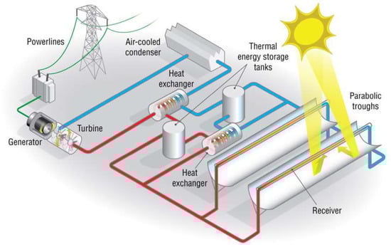
Figure 1.
System Advisor Model (SAM) sketch of a parabolic trough plant. Credit NREL/SAM.
The “physical” parabolic trough model is relatively complex involving a certain number of parameters to describe the different components. As such, there is uncertainty in prescribing all the geometric and operating parameters. The uncertainty at the components level translates into uncertainty at the system level. Tuning of the model vs. known plant operation is a necessary step before attempting any use of the model in designing new plants. Here the problem is that the experimental data to validate the models’ details, as well as the performance at the system level, are mostly missing. The “physical” parabolic trough model may include some transient effects, related to the thermal capacity of the heat transfer fluid, but it is certainly not expected to work well on short transients such as the passage of clouds, or, at least, it has never been validated towards transients.
A sample “physical” parabolic trough model of a solar facility for a 125 MW rated power and 6 hours of thermal energy storage located in Gila Bend is shown in Appendix A. The model is clearly very basic, describing the most part of the components by using simple equations plus empirical data.
Then, we attempt validation of the molten salt solar tower model in the same SAM Version 2018.11.11, updated to Revision 4, SSC 209. Also, in this case, we compare the monthly average results of experiments and simulations for the average year. In this case, there is one solar facility only to consider. The world’s largest concentrating solar power solar tower with thermal energy storage, the 110 MW Crescent Dunes, is also considered. Regarding the molten salt solar tower module, this is a semi-empirical model, less physically grounded than the “physical” parabolic trough model, and much more challenging. A sketch of a solar tower plant from SAM is shown in Figure 2.
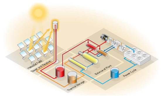
Figure 2.
SAM sketch of a solar tower plant. Credit NREL/SAM.
The central receiver system of concentrating solar power consists of a solar field of heliostats, a receiver atop of a central tall tower, the power block, and the optional thermal energy storage. Fossil fuel combustion for backup and ramp-up of operation is also an option. The solar field is made up of the many heliostats. They are flat, sun-tracking mirrors that focus the solar DNI onto the receiver atop of the tall tower. Thermal energy is collected by the heat transfer fluid heated in the receiver and delivered to the power block. Tracking is performed on two axes. The design is much more complicated vs. the parabolic trough collectors. It is more sensitive to wind-induced forces, and other environmental variables, and it does not produce, nor maintain, the much more challenging performances very easily. The distance between the heliostats and the central receiver is very large compared to the short distance of the parabolic trough mirror and collector. Every heliostat needs very careful and demanding control and misalignments are not uncommon. As an advantage, the power cycle is typically medium temperature steam, Rankine cycle, with typically also a slightly higher pressure to the turbine. The molten salt solar tower model is adapted from [28]. The heliostat solar field model is described in [28]. Receiver height and geometry, the geometry of heliostats and their layout in the solar field, and their optical, thermal and heat-transfer properties dictate the operation of the molten salt solar tower system. The heliostat solar field layout can be managed by using the code National Renewable Energy Laboratory (NREL) Solar PILOT Version 1.1 (National Renewable Energy Laboratory, 15013 Denver West Parkway, Golden, CO 80401, USA) [29]. This software permits the optimization of the position of every heliostat. The receiver model is based on semi-empirical equations. The receiver model is one of the weakest parts of the molten salt solar tower system model, as semi-empirical relations are dependent on the missing good experimental data. The semi-empirical equations for the receiver are proposed in [28]. The receiver is made up of a number of panels. Each panel consists of a set of parallel tubes in a common heat transfer fluid header. The heat transfer fluid flows through each panel in a serpentine. Despite the number of solar tower plants built and operated being minimal, there are many different options available for the heat-transfer fluid flow pattern through the receiver, such as a full circle or split path around the receiver, or split pass single cross-over.
There are similarities and differences with the “physical” parabolic trough model. The major difference is clearly the representation of the solar field and the receiver, which is definitively much more challenging in the molten salt solar tower model. Being semi-empirical, it requires more experimental support to work properly. Having less physical background, it may only work in a limited number of cases. If the real-world data of parabolic trough plants are limited, the real-world data of solar tower plants are in even shorter supply. Also considering the modeling of a solar tower system is much more challenging than a parabolic trough system, and the construction and operation of a solar tower system is much more challenging than the construction and operation of a parabolic trough system, the molten salt solar tower model should not be expected to work very well, being surely less accurate than the “physical” parabolic trough model. The molten salt solar tower model is much more complicated than the “physical” parabolic trough model, it presents a larger number of variants, it is less physical and more empirical, it necessitates a much larger number of good experimental data to work well over a limited number of circumstances.
A sample solar tower model of a solar facility for a 110 MW rated power and 10 hours of thermal energy storage located in Tonopah is shown in Appendix B. Also, this model is clearly very basic, describing most of the components by simple equations plus empirical data.
The validation exercises of SAM that have been performed so far were not exactly detailed validation exercises. In the specific section Concentrating Solar Power Validation [30], NREL reports about one parabolic trough and one solar tower studies performed with SAM 2013.1.15. Additionally, the only other study mentioned in the validation section of SAM is the recently published paper [31] on a solar tower study with SAM 2017.9.5. Also, this model is available for download in [32]. This is, however, a study on a plant “similar to Gemasolar” that only focuses on the short-term forecasts of DNI for plant operation without performing any comparison of experiments and simulations for what concerns the operation of the plant as a system and their components. This is not a validation.
One of the test cases is Andasol-1, a parabolic trough system in Aldeire, Spain [33,34]. As admitted in [34], real validation is missing. “Performance data from the plant is proprietary but even without a very accurate weather file the SAM model predicts an annual energy output and a PPA proportional to the values reported in the media”. Hence, a media “guess” of the electricity production over a year is used to validate the hourly operation of the solar facility by the model. The other test case is Gemasolar, a molten salt solar tower in Fuentes de Andalucia, Spain [35,36]. Also here a guess of the annual production is used as a single parameter for validation of the hourly electricity production over one year, as admitted in [36] by using the same sentence reproduced above. This is clearly not enough for a validation exercise.
These two “attempted” validation studies were performed by using only guesses of the annual electricity production as the single parameter to compare. The models developed are available for download in [33,35]. This is not an acceptable validation exercise. To address this major downfall, a study is performed here for the 3 largest concentrating solar power plants in the US not featuring natural gas burning. Genesis, Solana, and Mojave, all parabolic troughs, with monthly results of simulations compared to the experiments. No computations are performed for ISEGS, a solar tower plant featuring massive natural gas combustion, as the missing information about the natural gas combustion schedule is mandatory to understand the operation of the plant. Computations are performed for Crescent Dunes, the largest operational concentrating solar power solar tower in the US without natural gas combustion.
3. Results
3.1. Genesis (Blythe)
Data for Genesis is sourced from [37]. Figure 3 presents an image of Genesis. Figure 4 and Figure 5 are the computational and experimental results. Figure 4a is the computational thermal power produced by half the solar field and thermal power input to half the power cycle and Figure 4b is the computational net power output from one of the two turbines on the average day of every month. Figure 5 is the computed ε with a frequency every hour, and their daily and monthly averages, plus the experimental monthly average ε.
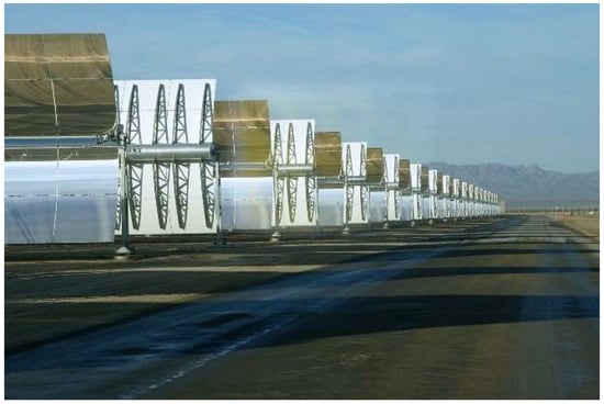
Figure 3.
Genesis solar facility. One image of the plant (from https://commons.wikimedia.org/wiki/File:Mirrors.JPG, CC-BY-SA-3.0).
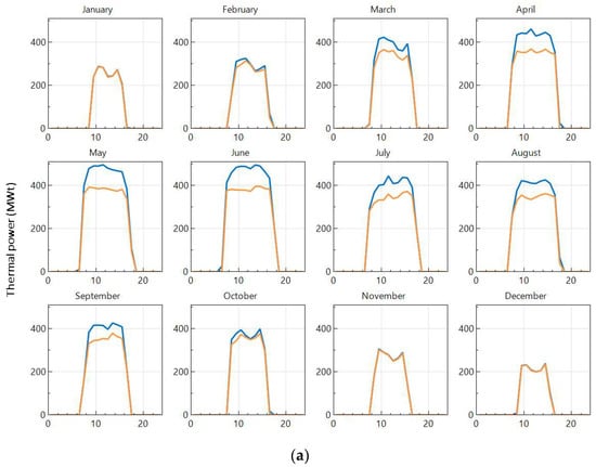
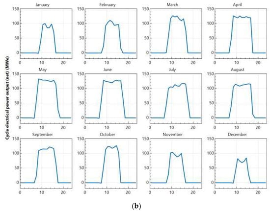
Figure 4.
Genesis solar facility. (a) Computational thermal power produced by half the solar field and thermal power input to half the power cycle and (b) computational net power output from one of the two turbines in the average day of every month. X is the time of the day in hours and Y the power in MW.
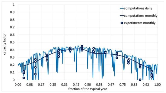
Figure 5.
Genesis solar facility. Daily and monthly capacity factors from computations and monthly capacity factors from experiments. X is the fraction of the year. Y is the capacity factor. The computation is made for the typical year. The experiments are the values measured since the completion of the plant (multiple entries per month).
Genesis is a concentrating solar power parabolic trough project. It includes two 125 MW power units. More than 500,000 parabolic mirrors are assembled in rows. The plant is located on 1950 acres close to Blythe, Riverside County, CA, US. The latitude and longitude location is 33°40′0.00″ North 114°59′0.00″ West. The electricity generation planned was 580,000 MWh/yr. The solar field is made up of 1480 Solar Collector Assemblies (SCAs), the number of loops is 460, the number of SCAs per loop is 4. The SCA manufacturer (model) is Sener (SenerTrough). The mirror manufacturer (Model) is Flabeg (RP3). The heat transfer fluid type is Therminol VP-1. The solar field inlet temperature is 293 °C. The solar field outlet temperature is 393 °C. The heat transfer fluid company is Solutia. The net turbine capacity is 250 MW by two turbines. The output type is steam Rankine, with a cooling method of a dry cooling, air-cooled condenser. There is no thermal energy storage. The pressure to the turbine is 100 bar.
Only half of the solar field is modeled, and 1 of the 2 turbines in the power block. The solar field is 779,674 m2. The power cycle has a design gross output of 140 MW. For an estimated gross to a net conversion factor of 0.895, the estimated net output at design (nameplate) is 125.30 MW. Note, the computed maximum generating power is in excess of the net turbine output for ε largely in excess of 1. Surprisingly, while the design gross output is 140 MW and the estimated net output at design (nameplate) is 125.30 MW, SAM computes values of the cycle electrical power output (net) from −7.44 MW to 160.65 MW.
The average year weather produces highs and lows fluctuations about the monthly averages that are reasonable. The seasonal variability is also well predicted. The computed monthly average values are always about the measured values, that suffer from about the same seasonal variability. Only in January are the model predictions significantly above the measurements, but this is only a minor departure from an otherwise well-predicted pattern. The latest experimental annual average ε is 0.28. Slightly higher annual average ε has been measured before, up to 0.29. The computational annual average ε, over the typical year, is 0.30. In the limit of an only low-frequency comparison with everything occurring overtime scales smaller than one month neglected, the agreement is satisfactory.
3.2. Mojave (Daggett)
Data for Mojave is sourced from [38]. The results for Mojave are presented in Figure 6 and Figure 7. Figure 6a is the computational thermal power produced by half the solar field and thermal power input to half the power cycle and Figure 6b is the computational net power output from one of the two turbines on the average day of every month. Figure 7 is the computed ε with a frequency every hour, and their daily and monthly averages, plus the experimental monthly average ε. Mojave is a concentrating solar power solar tower project located in Harper Dry Lake, San Bernardino County, CA, US. The latitude and longitude location is 35°1′0.00″ North 117°20′0.00″ West. As no weather data is available for this specific location, the weather data of Daggett are used. The land area is 1765 acres. The electricity generation expected 600,000 is MWh/yr. The solar field SCA manufacturer is Abengoa Solar. The mirror manufacturer is Rioglass. The HCE manufacturer (model) is Schott (PTR70). The heat-transfer fluid type is Therminol VP-1. The turbine capacity (net) is 250 MW by two turbines. The output type is steam, Rankine. The cooling method is wet cooling, cooling towers. There is no thermal energy storage. The pressure to the turbine is 100 bar, the same as Genesis. The temperature to and from the solar field is also the same as Genesis.
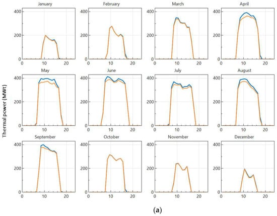
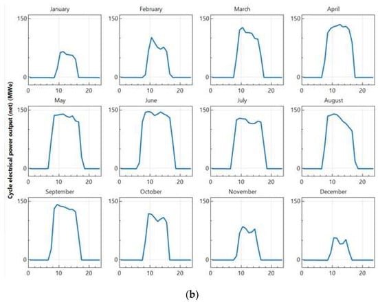
Figure 6.
Mojave solar facility. (a) Computational thermal power produced by half the solar field and thermal power input to half the power cycle. (b) Computational net power output from one of the two turbines in the average day of every month. X is the time of the day in hours and Y the power in MW.
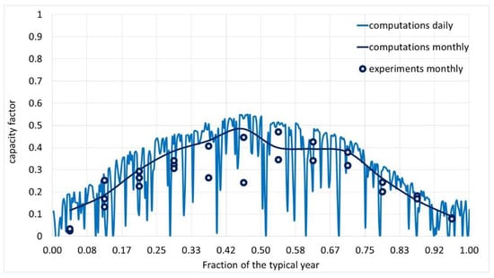
Figure 7.
Mojave solar facility. Daily and monthly capacity factors from computations and monthly capacity factors from experiments. X is the fraction of the year. Y is the capacity factor. The experiments are the values measured since the completion of the plant (multiple entries per month).
Only half of the solar field is modeled, and 1 of the 2 turbines in the power block. The solar field is 779,674 m2. The power cycle has a design gross output of 140 MW. For an estimated gross to a net conversion factor of 0.895, the estimated net output at design (nameplate) is 125.30 MW. Similarly, to Genesis, the computed maximum generating power is in excess of the net turbines’ output. The average year weather produces highs and lows about the monthly averages that are reasonable, as reasonable is the seasonal variation. The computed monthly average values are always about the measured values, which also suffers from seasonal variability. Only in January are the model predictions significantly above the measurements. The latest experimental annual average ε is 0.24 but a much higher annual average ε has been measured before, up to 0.29. The computational annual average ε over the typical year is 0.30. This is again a satisfactory agreement, as maintenance and other real-world issues may only detract from the computed performances.
3.3. Solana (Gila Bend)
Data for Solana is sourced from [39]. The results for Solana are presented in Figure 8 and Figure 9. Figure 8a is the computational thermal power produced by half the solar field, half the thermal energy storage power in and out, and thermal power input to half the power cycle and Figure 8b is the computational net power output from one of the two turbines in the average day of every month. Figure 9 is the computed ε with a frequency every hour, and their daily and monthly averages, plus the experimental monthly average ε. Solana is 70 miles from Phoenix, AZ. Thermal energy storage provides up to 6 hours of generating capacity after sunset. The land area is 780 hectares. The solar field aperture area is 2,200,000 m2. The number of SCAs is 3232. The number of loops is 808. The number of SCAs per loop is 4. The number of modules per SCA is 10. The receiver fluid is Therminol VP-1. The solar field inlet temperature is 293 °C. The solar field outlet temperature is 393 °C. The net capacity of the two turbines is 250 MW. The power cycle is steam Rankine with maximum pressure of 100 bar. The thermal energy storage is by 2-tank indirect, with a storage capacity of 6 hours using molten salt. The location is Gila Bend, Maricopa County, AZ, US. The latitude and longitude location is 32°55’0.00″ North 112°58’0.00" West. The electricity generation expected is 944,000 MWh/yr. The heat-transfer fluid company is Solutia.
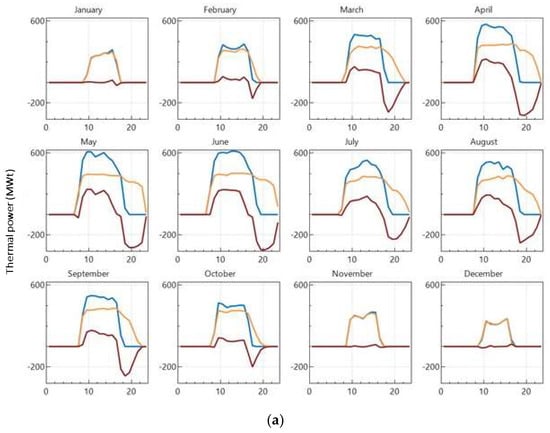
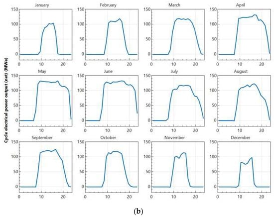
Figure 8.
Solana solar facility. (a) Computational thermal power produced by half the solar field, half the thermal energy storage power in and out, and thermal power input to half the power cycle. (b) Computational net power output from one of the two turbines in the average day of every month. X is the time of the day in hours and Y the power in MW.
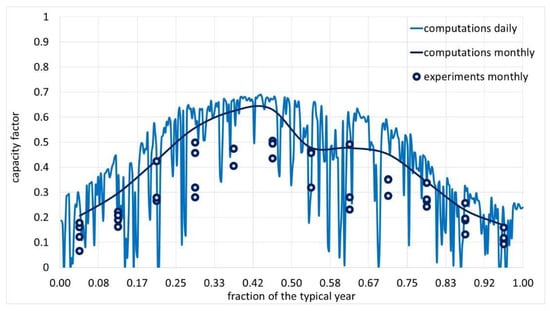
Figure 9.
Solana solar facility. Daily and monthly capacity factors from computations and monthly capacity factors from experiments. X is the fraction of the year. Y is the capacity factor. The experiments are the values measured since the completion of the plant (multiple entries per month).
Only half of the solar field is modeled, and 1 of the 2 turbines in the power block. The solar field is 1,100,000 m2. The power cycle has a design gross output of 140 MW. For an estimated gross to a net conversion factor of 0.895, the estimated net output at design (nameplate) is 125.30 MW. Compared to Genesis, and Mojave, of generally similar design parameters, apart from some changes in the size of the solar field, despite the same turbine output, the major difference is the thermal energy storage. The overrating of the maximum generating power is experienced also in this model. The average year weather produces reasonable highs and lows about the monthly averages that follow a reasonable seasonal pattern. The sharp decline of performances in June is well predicted. The delivered performances are on average 14% below the computational performances. The computed monthly average values are on average 14% larger than the measured values. The latest experimental annual average ε is 0.36. Only smaller annual average ε has been measured so far, as the learning curve for this kind of large solar plants is not completed. The computational annual average ε over the typical year is 0.41 (+14%). The impression (a population of 1 is insufficient to infer any proper statistic) is that, apart from operating issues due to the more complex design, the thermal energy storage module overrates the performance.
3.4. Crescent Dunes
Data for Crescent Dunes is sourced from [40,41,42,43]. An image of Crescent Dunes is presented in Figure 10. Figure 11a is the computational thermal power produced by the solar field, the thermal energy storage power in and out, and thermal power input to the power cycle and 11.b is the computational net power output from the turbine on the average day of every month. Figure 12 is the computed ε with a frequency every hour, and their daily and monthly averages, plus the experimental monthly average ε. The generation capacity is 110 MW net. The projected annual generation is 482,000 MWh (ε = 0.50) in [40], and more than 500,000 MWh (ε >0.52) in [41,42]. This electricity is calculated by using the project/NREL Technology specific ε. The plant is made up of 17,170 heliostat mirrors. The technology is a solar tower, the preferred technology supported by NREL. The location is Tonopah, NV, US. The latitude and longitude location is 38°14′20.00″ North, 117°21′48.00″ West.
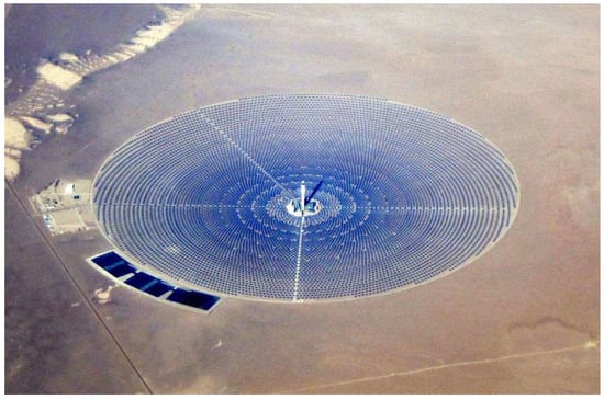
Figure 10.
Crescent Dunes solar facility. Image of the plant (from en.wikipedia.org/wiki/Crescent_Dunes_Solar_Energy_Project#/media/File:Crescent_Dunes_Solar_December_2014.JPG, CC BY-SA 4.0).
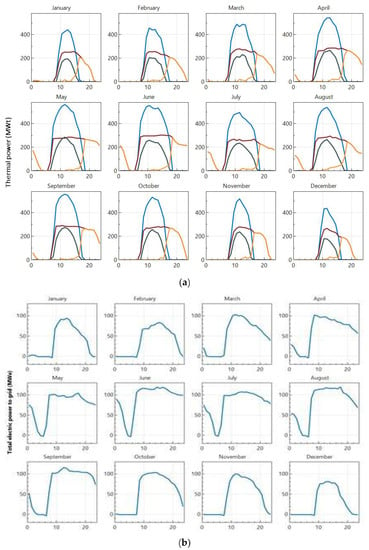
Figure 11.
Crescent Dunes solar facility. (a) Computational thermal power produced by the solar field, the thermal energy storage power in and out, and the thermal power input to the power cycle. (b) Computational net power output from the turbine in the average day of every month. The model for parabolic trough and the model for the solar tower have different outputs for the thermal energy storage. The solar tower has the charges and discharges separated. The parabolic trough has a single curve. X is the time of day in hours and Y the power in MW.
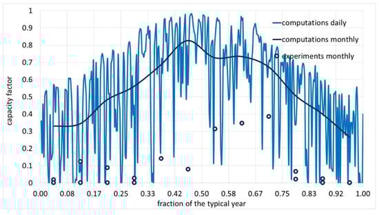
Figure 12.
Crescent Dunes solar facility. Hourly, daily and monthly capacity factors from computations and monthly capacity factors from experiments. X is the fraction of the year. Y is the capacity factor. The experiments are the values measured since the completion of the plant (multiple entries per month).
The land area is 1600 acres. The solar field heat transfer fluid type is molten salt. The heliostat solar field aperture area is 1,197,148 m2. The number of heliostats is 10,347. The heliostat aperture area is 115.7 m2. The tower height is 195 m. The receiver type is external–cylindrical. The receiver panel height (for the external receiver) is 30.48 m. The receiver inlet temperature is 288 °C. The receiver outlet temperature is 566 °C. The power block is characterized by a turbine of capacity (net) 110 MW. The steam Rankine power cycle has a maximum pressure of 115 bar. The cooling method is hybrid. Thermal energy storage is 2-tank direct, with storage capacity of 10 hours. Thermal energy storage is achieved by raising the molten salt temperature from 288 to 566 °C. Thermal energy storage efficiency is claimed to be 99%.
The heliostats’ reflective area is 1,161,235 m2. The power cycle has a design gross output of 122 MW. For an estimated gross to a net conversion factor of 0.9, the estimated net output at design (nameplate) is 109.8 MW. By contrast with Genesis, Mojave, and Solana, the design is a solar tower, and the same as Solana there is thermal energy storage, but larger. The higher pressure (115 vs. 100 bar) and the higher temperature (565 vs. 393 °C) are expected to translate in slightly higher efficiency of the power cycle. The computed efficiency is, however, much larger than any concentrating solar power parabolic trough facility considered, and this is due to the way the solar field and the collector are modeled, which is completely different from the parabolic trough model, and very likely fairly optimistic.
As with the parabolic trough models, the maximum computational ε are in excess of 1. The measured performances are dramatically below the computational performance. The computed monthly average ε are on average much larger than the measured values. The latest experimental annual average ε is 0.12. The largest 12 months’ average ε is 0.24. The computational annual average ε over the typical year is 0.54. This is more than double the experimental value. In no single month has the plant delivered the expected monthly ε. The impression (again, a population of 1 is insufficient to infer any proper statistic) is that the thermal energy storage module, as well as the solar field and collector models, overrate the performances, i.e., the sun’s energy collection is much less than what is assumed in the model and passing through the molten salt thermal energy storage, the energy lost is much more than what is modeled.
4. Discussion
The latest 12 months moving average of the capacity factor is 36.40% for Solana, 28.11% for Genesis, 24.45% for Mojave and 12.46% for Crescent Dunes. While the performances of Solana have been improving since the start of the operation, those for Genesis have been pretty much stable, while those for Mojave have been drastically reduced over the last 12 months by 4 percentage points from above 28% which is about the same as Genesis. Crescent Dunes has never been operational 12 months in a row, and not a single month has delivered the expected electricity production. The computational result from SAM is 30% for Genesis and Mojave, 41% for Solana, and 54% for Crescent Dunes. Solana is still suffering from some development issues, as demonstrated by the 12 months moving average increasing. The 5% percentage points of difference reflect the performance of some of the model components not reached yet in the real world. Crescent Dunes is conversely suffering from major development issues, as the differences are huge.
Concentrating solar power, especially solar tower, have performed so far much worse than the model predictions, while concentrating solar power parabolic trough model predictions have been much closer to the real-world operation. In particular, the example of the solar tower with thermal energy storage of Crescent Dunes, which has not delivered yet an annual average ε larger than 0.24, when the planned ε was >0.52, indicates the need for better models, with a more accurate representation of processes and components, to be finally properly validated. Real-world components seem to work differently from what is simplistically assumed in the models that are thus anything but accurate and reliable.
Things are much better with parabolic troughs than solar towers simply because it is much easier to operate a smaller number of single-axis reflectors focusing the sun on a central receiver, than to focus a multitude of two-axis reflectors on a small receiver atop of a tall tower that is very far from the reflectors, and similarly collect energy in the centralized receiver rather than the many receivers in every parabolic trough collector section. Additionally, the components of parabolic troughs have been studied more, this technology being much more widespread, and the model benefits from the feedback from real-world experiences, that are minimal with the solar tower. Furthermore, some of the environmental effects, for example, the effect of clouds, cannot be represented by simply using an average cloudiness factor, and full solar radiation, or simply an average DNI, and the solar tower definitively suffers from cloud transients much more than the parabolic trough. Similarly, the modeling of thermal energy storage is in need of a better definition, especially when the size of the storage increases.
What is needed for model development and validation is the availability of detailed experimental data, for both the operation of the plant and the environmental variables. A comparison of experiments and simulations with high-frequency sampling, every 1 min or less, as is requested for grid management, is mandatory to validate the simulations. Unfortunately, experimental data are difficult to find for the operation of concentrating solar power energy facilities. Similarly, it is difficult to source the weather data needed to describe the environmental conditions with the same frequency, which should also be simultaneous to the operation of the facility in order to serve model development and validation purposes. Without the high-frequency time series of operational parameters of the facilities and the weather conditions, there is no opportunity to develop accurate, reliable models.
5. Conclusions
The proposed validation of the latest SAM Version 2018.11.11, updated to Revision 4, SSC 209, vs. the experimental data of monthly electricity production for concentrating solar power parabolic trough and solar tower energy facilities, permits us to draw some conclusions. Figure 3, Figure 4, Figure 5 and Figure 6 permit us to assess the reliability of the solar field and receiver models for the solar tower and parabolic trough systems, as well as of the thermal energy storage models. Despite a much higher sampling frequency being needed to perform a proper validation, the exercise, the first of its kind for the latest concentrating solar power facilities, has significant reference value. The results of the simulations are relatively close to the measured operation for the parabolic trough, but very far from for the solar tower. Systematic errors in SAM must be corrected. The model of the solar field and receiver in the solar tower must be improved. Similarly, in need of improvement is the thermal energy storage model. Despite simple, the parabolic trough module is trustworthy. Some preliminary studies such as [44] can be attempted, but not full-scale design simulations, for parabolic trough installations. Further development of the SAM software, and the validation of this software vs. high-frequency data collected on the existing facilities, both for energy production, and weather conditions, is considered a necessary step before further progressing the design of novel concentrating solar power facilities by using this software. The relevance of good data monitoring is also discussed in [45]. The performance of the solar plant may change for any reason, linked to the variability of the resource, for example [46], as well as operation, maintenance, grid conditions, and many other causes, that need to be addressed. Lacking validation, SAM may only provide a very rough estimation of the power cycle output from a very rough estimation of the power cycle input from the solar field, and the charge and discharge of the thermal energy storage. SAM has outputs every hour of the year that have never been validated so far versus similarly detailed experiments, for both the resources, and the operation of the plant as a system and at the individual component level. SAM is a precious tool for the renewable energy community in general, and for those studying concentrated solar power in particular. It is now necessary to collect simultaneously high-frequency data of the resource and the weather conditions, as well as parameters detailing the operation of the system’s components and the total system output in order to perform a proper validation and refine the many semi-empirical models used in SAM. Once this necessary step is completed, then it will be possible to use SAM in designing new plants with reasonable confidence in the simulation results.
It must be added that concentrated solar power has a bright perspective that may only improve as soon as their design can improve through accurate, validated models. The advantages vs. PV are not only dispatchability, higher annual average capacity factor, a reduced standard deviation of the capacity factor, and production of electricity after sunset. Once a further evolved design can be proposed for an industrial product, mass production could then bring down the cost of kWh well below the value of PV, [8,9,10,11,12], which also needs batteries. Additionally, for the specific application in Saudi Arabia in general, but Al Khobar in particular, the enclosed trough with saltwater condenser suffers much less from sand, dust, humidity, salt and extreme temperatures than PV. PV in Saudi Arabia in general and Al Khobar in particular dramatically suffer from the above issues, [47,48,49] that are preventing the uptake of this technology. The panels collect much less solar energy, being quickly covered by a layer of dust, that is converted to less electricity also because of the high temperature. Additionally, failure of the panels also occurs due to rust and thermal-induced cracks. Better models may definitively accelerate the further progress of concentrated solar power.
The manuscript has proposed the best possible validation exercise of one of the best available software tools to model concentrated solar power plants, SAM. The validation is based on the best available data of electricity production from the US Energy Information Administration (EIA). Before this work, validation was improperly done by developing a model and comparing the annual model output with rumors from the general press of the output of 2 plants. With this work, validation is done by comparing high-quality electricity production data from the US EIA available monthly over multiple years with the 12-monthly results from the models developed in SAM for 5 plants. While much better data collected with a much higher frequency is certainly needed for a more proper validation, this exercise is certainly a giant step forward and, therefore, has reference value. The US EIA data are monthly values of very good quality, certainly the best in the world for concentrated solar power. Only the Australian Energy Market Operator (AEMO) data are possibly better, with data of contracts made available every 3 min. Unfortunately, Australia has no plant featuring this specific technology. The AEMO free market data properly satisfy every quality assurance requirement also through the auditing of buyers and sellers operations. The US EIA and the Australian AEMO are the best available measurements of electricity production and SAM is one of the best software tools developed to simulate the operation of concentrated solar power plants. Progress through further validation of detailed components as well as system operation sampled at high frequency is now a further step to permit better use of SAM in design and further uptake of concentrated solar power technology.
Author Contributions
A.B. and W.A.-K. collected the data, performed the simulations and compared the results of experiments and simulations. A.B., W.A.-K., and J.N. discussed the results and wrote the different sections of the manuscript. All authors have read and agreed to the published version of the manuscript.
Funding
This research received no external funding.
Conflicts of Interest
The authors declare no conflict of interest.
Appendix A. Sample “Physical” Parabolic trough Model of a Solar Facility for 125 MW Rated Power and 6 Hours of Thermal Energy Storage Located in Gila Bend
Here below are the input parameters. Highlighted are the parameters that are internally computed.


Appendix B. Sample Solar Tower Model of a Solar Facility for 110 MW Rated Power and 10 Hours of Thermal Energy Storage Located in Tonopah
Here below are the input parameters. Highlighted are the parameters that are internally computed.


References
- National Renewable Energy Laboratory, System Advisor Model (SAM)-NREL. 2019. Available online: sam.nrel.gov (accessed on 30 November 2019).
- Wagner, M. Modeling Parabolic Trough Systems. 2014. Available online: sam.nrel.gov/images/webinar_files/sam-webinars-2014-parabolic-trough-systems.pdf (accessed on 30 November 2019).
- Freeman, J.M.; DiOrio, N.A.; Blair, N.J.; Neises, T.W.; Wagner, M.J.; Gilman, P.; Janzou, S. System Advisor Model (SAM) General Description (Version 2017.9.5), NREL/TP-6A20-70414. 2018. Available online: www.nrel.gov/docs/fy18osti/70414.pdf (accessed on 30 November 2019).
- Wagner, M.J.; Zhu, G. Generic CSP Performance Model for NREL’s System Advisor Model: Preprint. NREL Report No. CP-5500-52473; 2011; 10p. Available online: http://www.nrel.gov/docs/fy11osti/52473.pdf (accessed on 30 November 2019).
- Kesseli, D.; Wagner, M.; Guédez, R.; Turchi, C. CSP-Plant Modeling Guidelines and Compliance of the System Advisor Model (SAM). DRAFT SolarPACES Conference Paper. 2018. Available online: Sam.nrel.gov/sites/default/files/content/documents/pdf/SolarPACES_2018_GuiSmo_DRAFT_v5.pdf (accessed on 30 November 2019).
- Wagner, M.J.; Gilman, P. Technical Manual for the SAM Physical Trough Model. NREL Report No. TP-5500-51825; 2011; p. 124. Available online: www.nrel.gov/docs/fy11osti/51825.pdf (accessed on 30 November 2019).
- Turchi, C.; Neises, T. Parabolic Trough Solar-Thermal Output Model Decoupled from SAM Power Block Assumptions. Milestone Report Prepared for the U.S. Department of Energy; 2015. Available online: Sam.nrel.gov/sites/default/files/content/user-support/DOE%20Milestone%20Report%20-%20Stand-alone%20Parabolic%20Trough%20code%202015-03-30.pdf (accessed on 30 November 2019).
- Boretti, A. Concentrated Solar Power Plants Capacity Factors: A Review, Nonlinear Approaches. In Engineering Applications Energy: Vibrations, and Modern Applications; Dai, L., Reza Jazar, N., Eds.; Springer: New York, NY, USA, 2018. [Google Scholar] [CrossRef]
- Boretti, A.; Castelletto, S.; Al-Zubaidy, S. Concentrating solar power tower technology: Present status and outlook. Nonlinear Eng. Model. Appl. (NLENG) 2018, 8. [Google Scholar] [CrossRef]
- Boretti, A. Cost and Production of Solar Thermal and Solar Photovoltaics Power Plants in the United States. Renew. Energy Focus. 2018, 26, 93–99. [Google Scholar] [CrossRef]
- Boretti, A.; Al-Zubaidy, S. A case study on combined cycle power plant integrated with solar energy in Trinidad and Tobago. Sustain. Energy Technol. Assess. 2019, 32, 100–110. [Google Scholar] [CrossRef]
- Boretti, A. Realistic expectation of electricity production from current design concentrated solar power solar tower with thermal energy storage. Energy Storage 2019, 1, e57. [Google Scholar] [CrossRef]
- Boretti, A. Energy storage requirements to address wind energy variability. Energy Storage 2019, 1, e77. [Google Scholar] [CrossRef]
- Boretti, A. Energy storage needs for an Australian National Electricity Market grid without combustion fuels. Energy Storage 2019. [Google Scholar] [CrossRef]
- Boretti, A. High-frequency standard deviation of the capacity factor of renewable energy facilities-part 1: Solar photovoltaic. Energy Storage 2019. [Google Scholar] [CrossRef]
- National Renewable Energy Laboratory. Concentrating Solar Power Projects by Project Name. 2019. Available online: www.nrel.gov/csp/solarpaces/by_project.cfm (accessed on 30 November 2019).
- Energy Information Administration. Electricity Data Browser-Plant Level Data. 2019. Available online: www.eia.gov/electricity/data/browser/ (accessed on 30 November 2019).
- Burkholder, F.; Kutscher, C. Heat Loss Testing of Schott’s 2008 PTR70 Parabolic Trough Receiver. National Renewable Energy Laboratory NREL/TP-550-45633; 2009. Available online: www.nrel.gov/docs/fy09osti/45633.pdf (accessed on 30 November 2019).
- Forristall, R. Heat Transfer Analysis and Modeling of a Parabolic Trough Solar Receiver Implemented in Engineering Equation Solver. National Renewable Energy Laboratory NREL/TP-550-34169; 2003. Available online: www.nrel.gov/csp/troughnet/pdfs/34169.pdf (accessed on 30 November 2019).
- Kelly, B.; Kearney, D. Parabolic Trough Solar System Piping Model. National Renewable Energy Laboratory NREL/SR-550-40165; 2006. Available online: www.nrel.gov/csp/troughnet/pdfs/40165.pdf (accessed on 30 November 2019).
- McMahan, A. Design & Optimization of Organic Rankine Cycle Solar-Thermal Power Plants. Master’s Thesis, University of Wisconsin-Madison, Madison, WI, USA, 2006. Available online: sel.me.wisc.edu/publications/theses/mcmahan06.zip (accessed on 30 November 2019).
- Moens, L.; Blake, D.M. Advanced Heat Transfer and Thermal Storage Fluids. National Renewable Energy Laboratory; NREL/CP-510-37083; 2005. Available online: www.nrel.gov/docs/fy05osti/37083.pdf (accessed on 30 November 2019).
- Patnode, A. Simulation and Performance Evaluation of Parabolic Trough Solar Power Plants. Master’s Thesis, University of Wisconsin-Madison, Madison, WI, USA, 2006. Available online: sel.me.wisc.edu/publications/theses/patnode06.zip (accessed on 30 November 2019).
- Pilkington Solar International GmbH. Survey of Thermal Storage for Parabolic Trough Power Plants. National Renewable Energy Laboratory; NREL/SR-550-27925; 2000. Available online: www.nrel.gov/csp/troughnet/pdfs/27925.pdf (accessed on 30 November 2019).
- Price, H.; Forristall, R.; Wendelin, T.; Lewandowski, A.; Moss, T.; Gummo, C. Field Survey of Parabolic Trough Receiver Thermal Performance. National Renewable Energy Laboratory NREL/CP-550-39459; 2006. Available online: www.nrel.gov/docs/fy06osti/39459.pdf (accessed on 30 November 2019).
- Stuetzle, T. Automatic Control of the 30 MWe SEGS VI Parabolic Trough Plant. Master’s Thesis, University of Wisconsin-Madison, Madison, WI, USA, 2002. Available online: sel.me.wisc.edu/publications/theses/Stuetzle02.zip (accessed on 30 November 2019).
- Troughnet Parabolic Trough Solar Power Network, National Renewable Energy Laboratory. 2019. Available online: www.nrel.gov/csp/troughnet (accessed on 30 November 2019).
- Wagner, T. Simulation and Predictive Performance Modeling of Utility-Scale Central Receiver System Power Plants. 2008. Available online: sel.me.wisc.edu/publications/theses/wagner08.zip (accessed on 30 November 2019).
- National Renewable Energy Laboratory. SolarPilot. 2019. Available online: www.nrel.gov/csp/solarpilot.html (accessed on 30 November 2019).
- National Renewable Energy Laboratory. CSP Validation. 2019. Available online: sam.nrel.gov/concentrating-solar-power/csp-validation.html (accessed on 30 November 2019).
- Lopes, F.; Ricardo Conceição, R.; Silva, H.; Fasquelle, T.; Salgado, R.; Canhoto, P.; Collares-Pereira, M. Short-Term Forecasts of DNI from an Integrated Forecasting System (ECMWF) for Optimized Operational Strategies of a Central Receiver System. Energies 2019, 12, 1368. [Google Scholar] [CrossRef]
- National Renewable Energy Laboratory. Gemasolar. 2017. Available online: sam.nrel.gov/images/web_page_files/molten-salt-tower-based-on-gemasolar-2017-9-5.sam (accessed on 30 November 2019).
- National Renewable Energy Laboratory. Available online: sam.nrel.gov/images/web_page_files/sam_case_csp_physical_trough_andasol-1_2013-1-15.zsam (accessed on 30 November 2019).
- National Renewable Energy Laboratory. Available online: sam.nrel.gov/images/web_page_files/sam_case_csp_physical_trough_andasol-1_2013-1-15.pdf (accessed on 30 November 2019).
- National Renewable Energy Laboratory. Available online: sam.nrel.gov/images/web_page_files/sam_case_csp_salt_tower_gemasolar_2013-1-15.zsam (accessed on 30 November 2019).
- National Renewable Energy Laboratory. Available online: sam.nrel.gov/images/web_page_files/sam_case_csp_salt_tower_gemasolar_2013-1-15.pdf (accessed on 30 November 2019).
- National Renewable Energy Laboratory. Genesis. 2019. Available online: solarpaces.nrel.gov/genesis-solar-energy-project (accessed on 30 November 2019).
- National Renewable Energy Laboratory. Mojave. 2019. Available online: solarpaces.nrel.gov/mojave-solar- (accessed on 30 November 2019).
- National Renewable Energy Laboratory. Solana. 2019. Available online: solarpaces.nrel.gov/solana-generating-station (accessed on 30 November 2019).
- Energy.gov. Crescent Dunes. 2019. Available online: www.energy.gov/lpo/crescent-dunes (accessed on 30 November 2019).
- Wang, A. Crescent Dunes Project Overview. 2014. Available online: www.leg.state.nv.us/App/InterimCommittee/REL/Document/5931?rewrote=1 (accessed on 30 November 2019).
- Crescent Dunes. 2019. Available online: www.power-technology.com/projects/crescent-dunes-solar-energy-project-nevada/ (accessed on 30 November 2019).
- National Renewable Energy Laboratory. Crescent Dunes. 2019. Available online: solarpaces.nrel.gov/crescent-dunes-solar-energy-project (accessed on 30 November 2019).
- Al-Kouz, W.; Nayfeh, J.; Boretti, A. Design of a parabolic trough concentrated solar power plant in Al-Khobar, Saudi Arabia. In Proceedings of the 6th International Conference on Renewable Energy Technologies (ICRET 2020), Perth, Australia, 8–10 January 2020. [Google Scholar]
- Beránek, V.; Olšan, T.; Libra, M.; Poulek, V.; Sedláček, J.; Dang, M.-Q.; Tyukhov, I.I. New Monitoring System for Photovoltaic Power Plants’ Management. Energies 2018, 11, 2495. [Google Scholar] [CrossRef]
- Libra, M.; Beránek, V.; Sedláček, J.; Poulek, V.; Tyukhov, I.I. Roof photovoltaic power plant operation during the solar eclipse. Sol. Energy 2016, 140, 109–112. [Google Scholar] [CrossRef]
- Al-Bashir, A.; Al-Dweri, M.; Al-Ghandoor, A.; Hammad, B.; Al-Kouz, W. Analysis of Effects of Solar Irradiance, Cell Temperature and Wind Speed on Photovoltaic Systems Performance. Int. J. Energy Econ. Policy 2020, 10, 353–359. [Google Scholar] [CrossRef]
- Al-Kouz, W.; Al-Dahidi, S.; Hammad, B.; Al-Abed, M. Modeling and analysis framework for investigating the impact of dust and temperature on PV systems’ performance and optimum cleaning frequency. Appl. Sci. 2019, 9, 1397. [Google Scholar] [CrossRef]
- Nader, N.; Al-Kouz, W.; Al-Dahidi, S. Assessment of Existing Photovoltaic System with Cooling and Cleaning System: Case Study at Al-Khobar City. Processes 2020, 8, 9. [Google Scholar] [CrossRef]


© 2020 by the authors. Licensee MDPI, Basel, Switzerland. This article is an open access article distributed under the terms and conditions of the Creative Commons Attribution (CC BY) license (http://creativecommons.org/licenses/by/4.0/).