Article

Real-Time Reconstruction of Contaminant Dispersion from Sparse Sensor Observations with Gappy POD Method

1
State Key Laboratory of Fluid Power and Mechatronic Systems, Zhejiang University, Hangzhou 310027, China
2
School of Mechanical Engineering, Zhejiang University, Hangzhou 310027, China
*
Author to whom correspondence should be addressed.
These authors contributed equally to this work.
Energies 2020, 13(8), 1956; https://doi.org/10.3390/en13081956
Submission received: 25 March 2020 / Revised: 9 April 2020 / Accepted: 11 April 2020 / Published: 15 April 2020
(This article belongs to the Special Issue Energy Efficiency and Indoor Environment Quality)

Abstract

:
Real-time estimation of three-dimensional field data for enclosed spaces is critical to HVAC control. This task is challenging, especially for large enclosed spaces with complex geometry, due to the nonuniform distribution and nonlinear variations of many environmental variables. Moreover, constructing and maintaining a network of sensors to fully cover the entire space is very costly, and insufficient sensor data might deteriorate system performance. Facing such a dilemma, gappy proper orthogonal decomposition (POD) offers a solution to provide three-dimensional field data with a limited number of sensor measurements. In this study, a gappy POD method for real-time reconstruction of contaminant distribution in an enclosed space is proposed by combining the POD method with a limited number of sensor measurements. To evaluate the gappy POD method, a computational fluid dynamics (CFD) model is utilized to perform a numerical simulation to validate the effectiveness of the gappy POD method in reconstructing contaminant distributions. In addition, the optimal sensor placement is given based on a quantitative metric to maximize the reconstruction accuracy, and the sensor placement constraints are also considered during the sensor design process. The gappy POD method is found to yield accurate reconstruction results. Further works will include the implementation of real-time control based on the POD method.

Graphical Abstract

1. Introduction

Automatic control of the HVAC system plays a significant role in improving indoor air [1,2,3,4] and reducing building energy consumption [5,6,7,8]. Real-time estimation of contaminant distribution inside any enclosed space could provide immediate feedback to the control of ventilation systems and, thus, is of great significance. However, the temporal evolution of contaminant distribution is characterized by complex nonlinear dynamics. It is challenging to reconstruct the spatiotemporal distribution of contaminants for real-time control of the ventilation system [9].
There are three main approaches to constructing indoor field data: spatial data interpolation, physics-based simulation, and the data-driven approach. Generally, ordinary Kriging is the most widely used spatial interpolation method [10] and could produce an effective estimate of an indoor thermal map [11] and pollutant distributions [11,12,13] based on sensor measurements. However, the accuracy of the interpolation is strongly dependent on sensor placements and the number of sensors. Typically, a large number of sensors are required to achieve adequate spatial resolution [11]. On another hand, physics-based models such as computational fluid dynamics (CFD) [14,15,16], fast fluid dynamics (FFD) [17,18,19,20,21,22], and zonal models [23,24,25] can provide three-dimensional field data for an indoor environment with only a small number of boundary conditions that are, however often difficult to obtain in real applications. Even though CFD have been widely employed for predicting the spatial variation of indoor environmental variables [26], the large amount of computational time makes real-time prediction extremely difficult and, thereby, unlikely to achieve real-time control. To overcome the large computational cost, the FFD model is proposed by solving the continuity equation and unsteady Navier-Stokes equations with a time-splitting approach [21]. In addition, the computational speed of FFD could be further accelerated by using parallel and GPU computing [19]. Considering its reasonable accuracy and high computational efficiency, the FFD method has been extensively studied for fast simulation of transient flow [18,19] and for inverse design of the ventilation parameters [20]. Although the reduction in computing time is significant, it is still computationally costly to implement, especially for real-time control. Different from CFD and FFD models, the zonal models are easily incorporated into the control system [25] and require very little computation time, because they only solve energy and mass balance equations at each thermal zone. However, based on the assumption that all quantities are uniform at each zone, zonal models are unable to provide detailed spatial information for a room space [23]. The third category is the data-driven approach. The artificial neural network (ANN) is one of the most widely used data-driven approaches for fast estimation of an indoor environment [27,28,29,30]. ANN models the nonlinear relationships between boundary conditions and environmental variables by training the data obtained from CFD simulations. However, an ANN model is very prone to over-fitting [12]. Moreover, as a black box model, it is difficult to interpret the results predicted by an ANN model.
Recently, the proper orthogonal decomposition (POD) has been extensively studied as a major class of data-driven approaches for dynamics reconstruction, since it provides a powerful tool to identify low-order modes of a system. Compared with ANN, POD provides a more interpretative reconstruction result by capturing the dominant physics-based coherent structures. At present, POD has wide application for dynamic reconstruction in the context of fluid mechanics [31,32], structural dynamics [33], ocean engineering [34,35], etc. As for the application in fluid dynamics, POD utilizes a few dominant POD bases for representation of the extracted flow features [36]. Moreover, to achieve active flow control in practice, sensor measurements must be introduced to the POD framework. Thus, gappy POD has been recently developed as an extension of the POD method by combining the POD model and sensor measurements [37]. Given a set of POD modes, gappy POD is able to reconstruct fluid dynamics with a limited number of sensor measurements through linear regression.
POD has recently been introduced to the field of built environment for fast reconstruction of the indoor temperature field [38,39,40,41,42,43] and airflow pattern [38,44]. For example, Allery et al. estimated the air flow pattern in a two-dimensional ventilated cavity by a POD-Galerkin construction [44]. Sempey et al. obtained reduced-order models of temperature distribution in an air-conditioned room under steady flow conditions based on the POD-Galerkin method [42]. Phan et al. applied the POD model for investigation of the temperature distribution in a data center by using the POD-Galerkin method and further investigated the effects of design parameters on the reconstruction accuracy [43]. Li et al. established a reduced-order model for fast estimation of the indoor thermal map by using Galerkin projection and further developed a real-time controller based on the reduced order model [41]. Tallet et al. used a POD model for real-time reconstruction of indoor temperature distribution based on sensor measurements [38]. Meyer et al. combined the POD method with the linear stochastic estimation method for reconstruction of the fluctuating thermal field in an experimental room based on real-time sensor measurements [40]. Jiang et al. fuse the input parameters of a CFD simulation and sparse sensor observations for reconstruction of a steady indoor thermal field [39]. However, gappy POD, which has been confirmed to perform well in turbulent flow sensing [37,45], has seldom been used for reconstructing the transient variations of the indoor environment.
Sensor measurements are critical to the estimation and control of the indoor environment. Considering the nonuniform distribution of indoor contaminants, a large number of sensors are required to guarantee satisfactory HVAC performance, which, however, is usually cost-expensive. Thus, it is of great significance to extrapolate the three-dimensional distribution of indoor air contaminants based on limited sensor measurements. In this paper, a gappy POD method for the real-time reconstruction of contaminant distribution in an enclosed space is proposed by combining the POD method with a limited number of sensor measurements. Even though gappy POD has been confirmed to perform well in the field of turbulent flow sensing, the effects of gappy POD on the real-time reconstruction of contaminant distributions remain to be investigated. To evaluate the effects of gappy POD for the reconstruction of indoor environments, CFD models are utilized to perform the simulation study to validate the reconstruction results. The article is organized as follows. Section 2 briefly introduces the gappy POD method and the algorithm for optimal sensor placement. The reconstruction results of the contaminant distribution are presented in Section 3. Finally, the main conclusions are presented in Section 4.

2. Materials and Methods

2.1. Standard POD

The spatiotemporal distribution of contaminants is characterized by complex nonlinear dynamics. The POD method provides a powerful tool to decompose the high-dimensional dynamics to basic POD modes for representation of the coherent structures for contaminant distribution. The snapshot method was introduced by Sirovich et al. for determination of the basic POD modes [46]. The snapshots X are formed by collecting the time-series data.
X = [ x ( t 1 ) x ( t 2 ) x ( t k ) x ( t m ) ]
where x ( t k ) is a vector of n elements representing the spatial distribution of the contaminants at a time t k . The snapshot x ( t k ) could be obtained from CFD simulation results. The correlation matrix R of size m × m is defined by
R = 1 m   X T X
Then, the eigenvectors φ = [ φ 1 , φ 2 , φ m ] of the correlation matrix R, and its corresponding eigenvalues λ = [ λ 1 , λ 2 , λ m ] are computed. The basic POD modes ϕ is given by a linear combination of snapshots
ϕ j = X φ j X φ j 2
where φ j denotes the j t h eigenvector. The eigenvalue is ordered in terms of the importance of their corresponding POD modes ( λ 1 > λ 2 > λ 3 > λ m ). The lager eigenvalue means that the corresponding basic POD modes plays a more important role in describing the contaminant distribution. By using the first p eigenvectors, the contaminant concentration could be reconstructed as
x i = 1 p b i Φ i
where b i are temporal coefficients of the i t h POD basis mode, and x is the vector representing the estimation of contaminant distribution in the enclosed space. For POD applications, the most important issue is the determination of the coefficients for basic POD modes.

2.2. Gappy POD

Gappy POD provides an effective method for the calculation of POD coefficients based on sparse sensor observations. The mask vector H of the n elements records the sensor locations. If the sensor is located on the ith grid point, then the ith element in H is equal to one; otherwise, the ith element in H is equal to zero. The incomplete vector x of the n elements describes the contaminant concentration at n locations corresponding to sensor locations but also has some elements missing. The full vector x ˜ of the n elements represents the reconstructed contaminant concentration. The gappy POD could reconstruct the full vector x ˜ from the incomplete vector x . The POD coefficient could be obtained by solving a linear regression in Equation (5).
M b ˜ = f
where
M i j = ( ( H , Φ i ) , ( H , Φ j ) )
and
f i = ( x , ( H , Φ i ) )
The coefficient b ˜ could be obtained by solving Equation (5), and the spatial distribution of contaminants could be immediately reconstructed through Equation (4).

2.3. Sensor Placement

According to Equation (5), the POD coefficient is obtained through data regression. The condition number of matrix M is a good proxy for evaluating the solution accuracy of Equation (5). The smaller condition number could contribute to the higher solution stability for Equation (5). The optimal sensor placement for the N sensors could be determined by the following equations:
min κ ( M ) s . t .   K ( i , 1 )   ϵ   { 0 , 1 } ,   i = 1 , 2 , , n j = 1 n K ( i , 1 ) = N
where κ ( M ) is the condition number of M.
The sensor placement could be obtained based on a greedy algorithm to minimize κ ( M ) [37]. Firstly, loop over all possible placement points, evaluate the condition number of M for each point, and choose the point that minimizes κ(M) to locate the first sensor. Then, determine the location of the next sensor that could minimize the condition number κ ( M ) . Repeat the previous steps until all the N sensors are placed in appropriate locations. For sensors with placement constraints, the number of possible sensor placement points would be fewer, and the only change we have to make is to loop over locations within location constraints for the optimal sensor placement.

2.4. Numerical Model

In the present study, the turbulent model based on Reynolds-Averaged Navier Stokes (RANS) is adopted. According to the previous studies focusing on gaseous contaminant dispersion in an enclosed space, the Eulerian method is able to provide an effective solution for simulating an indoor concentration distribution [26,47]. Therefore, the Eulerian method is used to predict the contaminant distributions in this study. Moreover, it is assumed that there is no chemical reaction during the gaseous contaminant dispersion process.
The experimental results given by Yuan et al. were utilized to validate the reliability of our numerical model [48]. The experiments were conducted in a test chamber with a size of 5.16 m × 3.65 m × 2.43 m (length × width × height) under the displacement ventilation. The total flow rate was 0.05 m3/s. The supply inlet was placed at the middle of the side wall near the floor, and the exhaust device of size 0.43 m × 0.43 m was fixed at the center of the ceiling. Two heated manikins, two computers, and six lamps were used to simulate heat sources. SF6 was used to simulate contaminants from occupants, and the contaminant source was placed above the simulated occupants.
Figure 1 gives the comparisons of the velocity and dimensionless SF6 concentration profiles between the numerical results and the experimental data. It could be observed that the agreement between the CFD results and the experimental data is reasonably good. Discrepancies between the simulated results and experimental values could be observed in the upper part of the space. Additionally, the discrepancies could also be found in the simulation study by Yuan et al. [49], who conducted this experiment and explained that this was because of recirculating flows in the upper part of the space. Moreover, it should be noted that the uncertainties for the experimental data are 0.01 m/s and 10% for the SF6 concentration [49].

2.5. Model Setup

In this study, the case is set in an enclosed space with dimensions of 4 m (L) × 3 m (W) × 2.5 m (H). Both airflow inlet and outlet are located on the left wall with dimensions of 0.6 m × 0.3 m. The inlet is located in the upper part of the left-side wall of 0.3 m beneath the ceiling, while the outlet is located in the lower part of the left-side wall of 0.3 m above the floor. A gaseous contaminant source is located in the center of the room. Detailed configurations of the ventilation system are shown in Figure 2. Moreover, the sensor locations are assumed to be constrained on the left and the back wall.
The reconstruction of the contaminant distribution is decomposed into two steps: the offline stage and online stage (Figure 3). In the offline stage, the snapshots are decomposed into basic POD modes, and the optimal sensor placement is determined. In the online stage, the temporal coefficients for POD modes are obtained based on the sparse sensor measurements through linear regression and then are applied for reconstruction of the contaminant distribution through a linear combination of the dominant POD modes. The POD-based online-offline algorithm has already been applied to many cases for optimal control of the dynamic systems, including optimal control of the water flooding reservoir [50] and optimal control of the indoor temperature [38,41]. The detailed procedure is described as follows:
(1) Collect a set of snapshots with a combination of different inlet velocities and contaminant source strengths. In case I, we first obtain the steady contaminant distribution with the CFD model for an inlet velocity of 1 m/s, and the gaseous contaminant is steadily released with a source strength of 1 mL per cubic meter per second. Using the steady contaminant distribution as the initial condition, the inlet velocity experiences a step change from 1 m/s to 2 m/s, and the source strength remains unchanged. The simulation results are recorded as snapshots until the next steady state is reached. In summary, the snapshots are recorded every 1 s, and 180 snapshots are obtained during the response process in case I. Case II follows a similar procedure as case I; the only difference between case I and case II is that the gaseous contaminant is steadily released with a source strength of 2 times higher than the source strength in case I. A sum of 320 snapshots are recorded for case II. Finally, a snapshot matrix combining the snapshots in both case I and case II is formed.
(2) Decompose the snapshots to obtain the POD modes, and then the optimal senor placement can be determined by minimizing the condition number in Equation (8). Moreover, it should be noted that the number of sensors should be more than the number of the dominant POD modes to make sure that the optimal algorithm for sensor placement is not an underdetermined problem.
(3) In the online stage, the temporal coefficients of the POD modes are determined based on the real-time measurements from the sparse sensors. The CFD simulations in the test case are used to provide sensor observations for implementing gappy POD reconstruction and to validate the reconstruction results. In particular, it is noteworthy that the gappy POD in the online step does not rely on any CFD simulation, and the CFD simulation here is used to perform a simulation study to evaluate the gappy POD model. The test case is set when the contaminant is steadily released at a source strength of 1.5 times higher than the source strength in case I. We first obtain the steady contaminant distribution with the CFD model for an inlet velocity of 1.2 m/s, and then, the inlet velocity is subject to a 0.4 m/s positive step to 1.6 m/s. The gappy POD method can be applied for reconstruction of the contaminant distribution in this test case, because the airflow pattern in our test case shares similar coherent structures with the snapshots. Moreover, Sempey et al. confirmed that the POD method performs well in reconstructing system dynamics with boundary conditions different from the conditions used for constructing snapshots [42].
(4) Reconstruct the spatiotemporal distribution of the contaminants based on the basic POD modes and the corresponding temporal coefficients.

3. Results

3.1. POD Decomposition

The snapshots of the contaminant distributions are of great importance for characterizing the system dynamics, and the dominant POD modes are built based on the snapshot ensemble. In detail, the contaminant is released from the center of the enclosed space, and the concentration is highest around the contaminant source. The contaminant distribution evolves with time as a response to the step increase of the inlet velocity from 1 m/s to 2 m/s.
A total of 500 POD modes and 500 corresponding eigenvalues are obtained based on the POD decomposition process. The exponential decay of the normalized eigenvalues is demonstrated in Figure 4. The normalized eigenvalues are calculated by dividing the sum of the total 500 eigenvalues and are regarded as a significant parameter for evaluating the percentage of energy contained in their corresponding POD modes and for measuring the importance of the POD modes. The normalized eigenvalues in Figure 4 are ordered in terms of their ability to describe the spatiotemporal distribution of the contaminants. It could be observed that the first few modes account for most of the system’s energy. For example, the first, second, and third POD mode accounts for 66.63%, 17.83%, and 4.26% of the total system energy, respectively. In addition, the first six POD modes contain about 95% of the total system energy, while the first 16 POD modes contain about 99% of the total system energy. As the normalized eigenvalue decreases, the corresponding POD mode will exhibit less meaningful spatial structures and contribute less to reconstructing the contaminant dispersion process.

3.2. Sensor Placement

It is challenging to optimize the sensor placement to maximize the reconstruction accuracy, since there are thousands of potential locations for sensor placement. A quantitative framework is used to determine the sensor locations by minimizing the condition number of the M matrix in Equation (8). The sensor locations are assumed to be constrained on the left and the back wall. For example, the optimal sensor placements of 20 sensors with location constraints is demonstrated in Figure 5. The potential sensor location could be in any location of the approximately 3000 grids on the left and the back wall. The optimization strategy is to pick up 20 points from the 3000 potential locations for the placement of sensors that could minimize the condition number of M in Equation (8) based on the greedy algorithm. It should be noted that increasing the POD mode number or increasing the sensor number would both result in a higher computational cost for finding the optimal sensor location. However, the computation of the optimal sensor placement is in the off-line stage and would not affect the speed for the real-time contaminant reconstruction in the online stage. Moreover, it can be observed that the sensors with location constraints are always kept away from the contaminant source. This can benefit the sensors by protecting them from long-term exposure to high-concentration contaminants and can improve the sensors’ service lives.

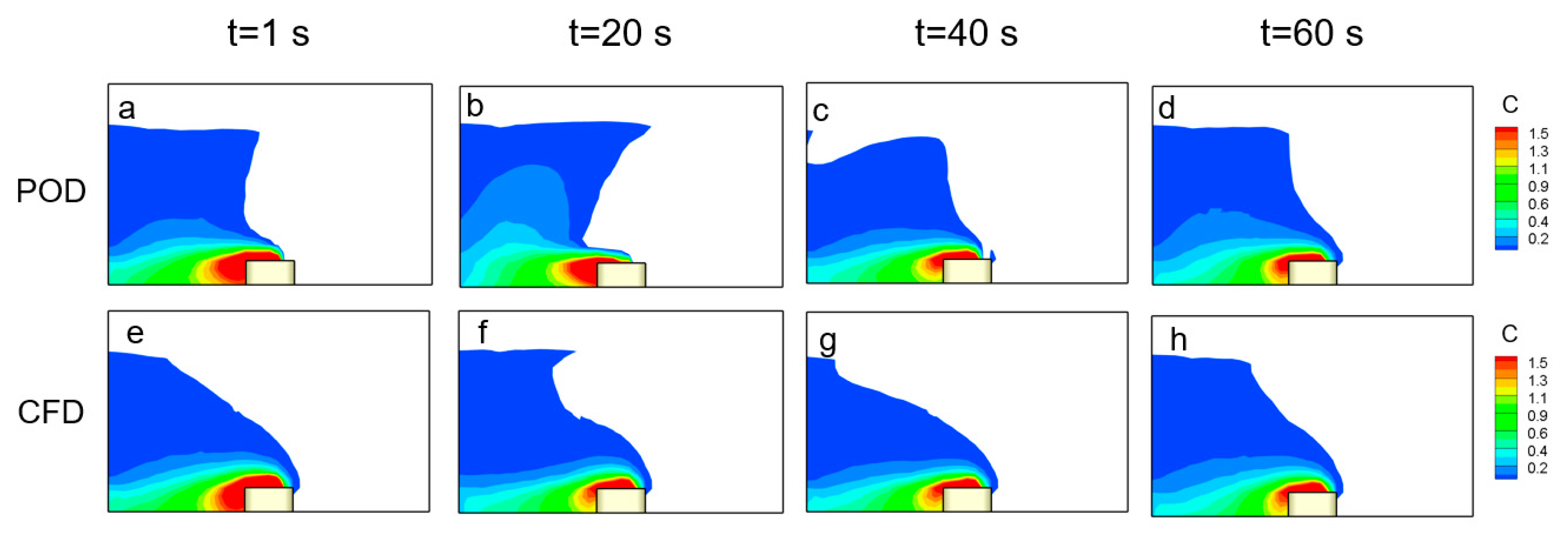
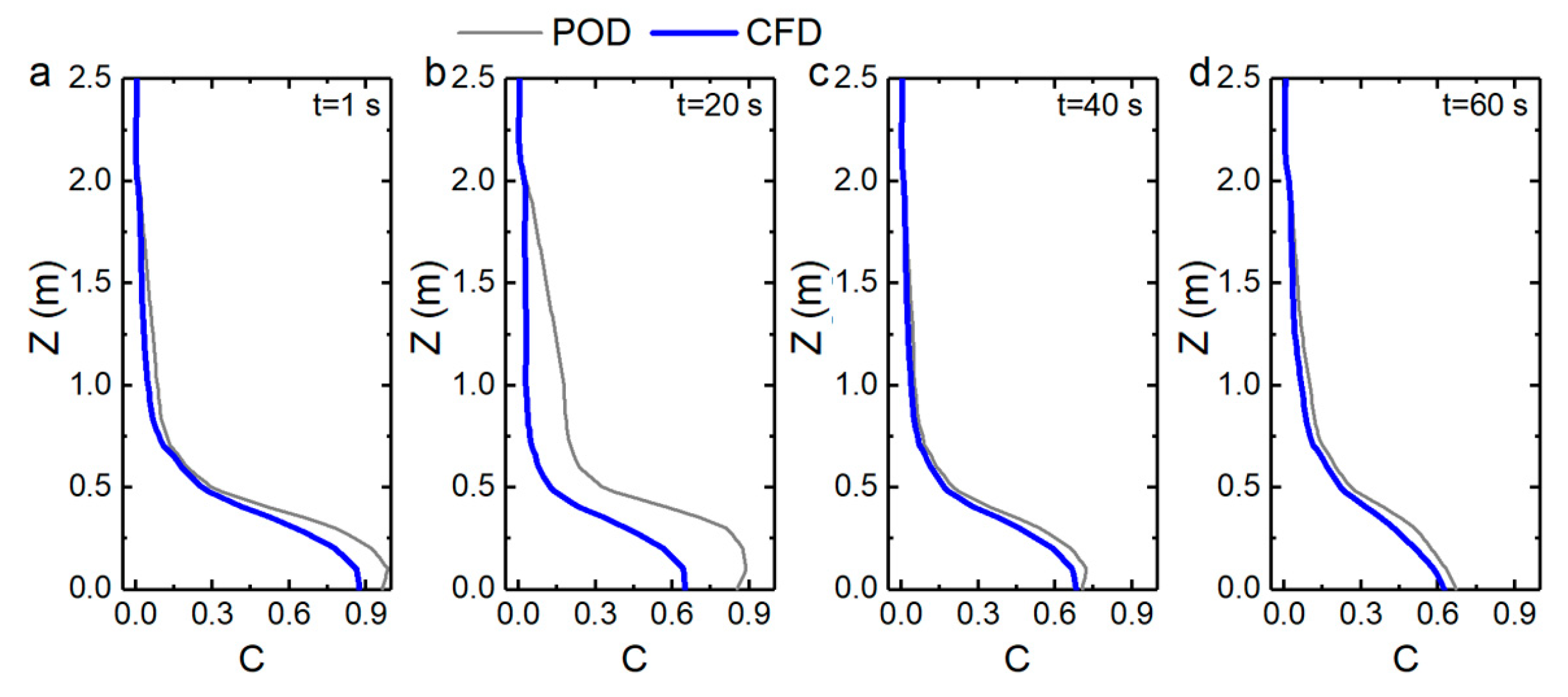
3.3. Gappy Flow Reconstruction

Quantifying the indoor air quality plays an important role in analyzing indoor occupant exposure [51]. Figure 6 demonstrates the estimation of the contaminant distribution based on 16 dominant POD modes with sensor placement constraints. It should be noted that the reconstruction accuracy is significantly limited by the number of dominant POD modes chosen for estimation of the contaminant distribution, and the first 16 modes contain more than 99% of the total system energy. As shown in Figure 6, the gappy POD method exhibits a high reconstruction accuracy and performs extremely well in estimating a contaminant concentration higher than 0.02 ppm. This is because 16 POD modes could capture a sufficiently detailed structure for reconstruction of the contaminant dispersion process. Moreover, the difference between gappy POD reconstruction and CFD simulation can be observed at t = 20 s, because it is difficult to reconstruct the contaminant distribution during this period with dramatical variations in the airflow field.
For further evaluation of the gappy POD method, comparison of the estimated contaminant concentration along the line x = 1.5 m, y = 1 m is conducted (Figure 7). The difference between the POD reconstruction and CFD simulation could be observed at t = 20 s due to the slightly different airflow pattern from the snapshots, which could also be observed in Figure 6. However, the gappy POD performs well in most conditions, because the airflow pattern in our test case shares similar coherent structures with snapshots in most conditions. Moreover, Sempey et al. confirmed that the POD method performs well in reconstructing system dynamics with boundary conditions different from the conditions used for constructing snapshots [42].
The reconstruction accuracy could be improved by increasing the dominant POD modes. This is because more POD modes can contribute to more detailed information for the description of the pollutant distribution. In our study, we found that 16 dominant POD modes are sufficient for estimation of the contaminant distribution in the enclosed space with sensor placement constraints.

4. Discussions and Conclusions

Real-time estimation of the contaminant distribution is essential for ventilation control and indoor air quality management. Moreover, it is known that automatic control is of great importance for improving a systems’ energy efficiency in engineering applications [52,53,54,55]. However, it is challenging to reconstruct spatiotemporal distributions of contaminants in an enclosed space, due to the ununiform distribution and nonlinear variations of indoor contaminants. As an essential part of active control, the sensor measurements only provide limited information about contaminant concentrations near sensor locations. Usually, a large number of sensors are required to guarantee the satisfactory performance of HVAC control, which might result in high costs for maintaining and conducting a sensor network in practice. Facing such a dilemma, the gappy POD offers a solution to provide real-time contaminant distributions with a limited number of sensor measurements.
In this study, a gappy POD method for the real-time reconstruction of pollutant distribution in an enclosed space is proposed by combining the POD method with a limited number of sensor measurements. In fact, the spatial distribution of indoor contaminants is often represented by a combination of a few dominant patterns, and this inherent property enables reconstruction of the contaminant distribution with sparse sensor observations. Moreover, our study gives the optimal sensor placement based on a quantitative metric in order to maximize the reconstruction accuracy. The sensor placement constraints are also considered during the sensor design process. It should be noted that the reconstruction accuracy is significantly limited by the number of dominant POD modes chosen for estimation of the pollutant distributions. For example, the first six POD modes only contain about 95% of the total system energy, while the first 16 POD modes contain about 99% of the total system energy. According to our study, reconstruction based on 16 POD modes are sufficient for accurate reconstruction of the pollutant distribution in the enclosed space.
For feedback control of the HVAC, gappy POD is able to provide a reliable estimation of three-dimensional data for the indoor environment with a high fidelity and low computational cost. Considering the low-order nature of the POD model, a closed-loop control might be achieved by controlling the coefficient of the POD modes, and the estimated POD coefficients could provide the necessary information for driving the HVAC actuators. Further work will include real-time control of the dynamic system based on the gappy POD method.

Author Contributions

Y.L.: conceptualization, methodology, and writing—original draft preparation. Z.T.: methodology, project administration and writing—review and editing. All authors have read and agreed to the published version of the manuscript.

Funding

This work was supported by the National Natural Science Foundation of China (51708493); Zhejiang Provincial Natural Science Foundation (LR19E050002); the National Key R&D Program of China (grant no. 2019YFB2004604); the Zhejiang Province Key Science and Technology Project (2018C01020, 2018C01060, and 2019C01057); and the Youth Funds of State Key Laboratory of Fluid Power & Mechatronic Systems (SKLoFP_QN_1804).

Conflicts of Interest

The authors declare no conflict of interest.

References

  1. Lim, E.; Ito, K.; Sandberg, M. Performance evaluation of contaminant removal and air quality control for local ventilation systems using the ventilation index Net Escape Velocity. Build. Environ. 2014, 79, 78–89. [Google Scholar] [CrossRef]
  2. Kolokotsa, D.; Pouliezos, A.; Stavrakakis, G.; Lazos, C. Predictive control techniques for energy and indoor environmental quality management in buildings. Build. Environ. 2009, 44, 1850–1863. [Google Scholar] [CrossRef]
  3. Lee, S.; Hwangbo, S.; Kim, J.T.; Yoo, C.K. Gain scheduling based ventilation control with varying periodic indoor air quality (IAQ) dynamics for healthy IAQ and energy savings. Energy Build. 2017, 153, 275–286. [Google Scholar] [CrossRef]
  4. Tong, Z.; Chen, Y.; Malkawi, A.; Liu, Z.; Freeman, R.B. Energy saving potential of natural ventilation in China: The impact of ambient air pollution. Appl. Energy 2016, 179, 660–668. [Google Scholar] [CrossRef] [Green Version]
  5. Cao, Y.; Du, J.; Soleymanzadeh, E. Model predictive control of commercial buildings in demand response programs in the presence of thermal storage. J. Clean. Prod. 2019, 218, 315–327. [Google Scholar] [CrossRef]
  6. King, J.; Perry, C. Smart Buildings: Using Smart Technology to Save Energy in Existing Buildings; Amercian Council for an Energy-Efficient Economy: Washington, DC, USA, 2017. [Google Scholar]
  7. Hu, S.; Hoare, C.; Raftery, P.; O’Donnell, J. Environmental and energy performance assessment of buildings using scenario modelling and fuzzy analytic network process. Appl. Energy 2019, 255, 113788. [Google Scholar] [CrossRef]
  8. Li, K.; Su, H. Forecasting building energy consumption with hybrid genetic algorithm-hierarchical adaptive network-based fuzzy inference system. Energy Build. 2010, 42, 2070–2076. [Google Scholar] [CrossRef]
  9. Manohar, K.; Brunton, B.W.; Kutz, J.N.; Brunton, S.L. Data-Driven Sparse Sensor Placement for Reconstruction: Demonstrating the Benefits of Exploiting Known Patterns. IEEE Contr. Syst. Mag. 2018, 38, 63–86. [Google Scholar]
  10. Burrough, P.A.; McDonnell, R.; McDonnell, R.A.; Lloyd, C.D. Principles of Geographical Information Systems; Oxford University Press: Oxford, UK, 2015. [Google Scholar]
  11. Huang, Y.; Shen, X.; Li, J.; Li, B.; Duan, R.; Lin, C.H.; Chen, Q. A method to optimize sampling locations for measuring indoor air distributions. Atmos. Environ. 2015, 102, 355–365. [Google Scholar] [CrossRef]
  12. Li, J.; Li, H.; Ma, Y.; Wang, Y.; Abokifa, A.A.; Lu, C.; Biswas, P. Spatiotemporal distribution of indoor particulate matter concentration with a low-cost sensor network. Build. Environ. 2018, 127, 138–147. [Google Scholar] [CrossRef]
  13. Cheng, K.-C.; Tseng, C.-H.; Hildemann, L.M. Using Indoor Positioning and Mobile Sensing for Spatial Exposure and Environmental Characterizations: Pilot Demonstration of PM2. 5 Mapping. Environ. Sci. Technol. Lett. 2019, 6, 153–158. [Google Scholar] [CrossRef]
  14. Kosutova, K.; van Hooff, T.; Vanderwel, C.; Blocken, B.; Hensen, J. Cross-ventilation in a generic isolated building equipped with louvers: Wind-tunnel experiments and CFD simulations. Build. Environ. 2019, 154, 263–280. [Google Scholar] [CrossRef]
  15. Aganovic, A.; Steffensen, M.; Cao, G. CFD study of the air distribution and occupant draught sensation in a patient ward equipped with protected zone ventilation. Build. Environ. 2019, 162, 106279. [Google Scholar] [CrossRef]
  16. Liu, W.; Liu, D.; Gao, N. CFD study on gaseous pollutant transmission characteristics under different ventilation strategies in a typical chemical laboratory. Build. Environ. 2017, 126, 238–251. [Google Scholar] [CrossRef]
  17. Zuo, W.; Chen, Q. Real-time or faster-than-real-time simulation of airflow in buildings. Indoor Air 2009, 19, 33. [Google Scholar] [CrossRef] [Green Version]
  18. Zuo, W.; Chen, Q. Fast and informative flow simulations in a building by using fast fluid dynamics model on graphics processing unit. Build. Environ. 2010, 45, 747–757. [Google Scholar] [CrossRef]
  19. Zuo, W.; Chen, Q. Simulations of Air Distributions in Buildings by FFD on GPU. HVAC&R Res. 2010, 16, 785–798. [Google Scholar]
  20. Xue, Y.; Liu, W.; Wang, Q.; Bu, F. Development of an integrated approach for the inverse design of built environment by a fast fluid dynamics-based generic algorithm. Build. Environ. 2019, 160, 106205. [Google Scholar] [CrossRef]
  21. Liu, W.; Jin, M.; Chen, C.; You, R.; Chen, Q. Implementation of a fast fluid dynamics model in OpenFOAM for simulating indoor airflow. Numer. Heat Transf. Part A Appl. 2016, 69, 748–762. [Google Scholar] [CrossRef]
  22. Jin, M.; Zuo, W.; Chen, Q. Improvements of Fast Fluid Dynamics for Simulating Air Flow in Buildings. Numer. Heat Transf. Part B Fundam. 2012, 62, 419–438. [Google Scholar] [CrossRef]
  23. Megri, C.A.; Haghighat, F. Zonal modeling for simulating indoor environment of buildings: Review, recent developments, and applications. HVAC&R Res. 2007, 13, 887–905. [Google Scholar]
  24. Jiru, E.T.; Haghighat, F. Modeling ventilated double skin façade—A zonal approach. Energy Build. 2008, 40, 1567–1576. [Google Scholar] [CrossRef]
  25. Song, Z.; Murray, B.T.; Sammakia, B. A dynamic compact thermal model for data center analysis and control using the zonal method and artificial neural networks. Appl. Therm. Eng. 2014, 62, 48–57. [Google Scholar] [CrossRef]
  26. Chen, Q. Ventilation performance prediction for buildings: A method overview and recent applications. Build. Environ. 2009, 44, 848–858. [Google Scholar] [CrossRef]
  27. Song, Z.; Murray, B.T.; Sammakia, B. Airflow and temperature distribution optimization in data centers using artificial neural networks. Int. J. Heat Mass Transf. 2013, 64, 80–90. [Google Scholar] [CrossRef]
  28. Cao, S.-J.; Ren, C. Ventilation control strategy using low-dimensional linear ventilation models and artificial neural network. Build. Environ. 2018, 144, 316–333. [Google Scholar] [CrossRef]
  29. Zhou, L.; Haghighat, F. Optimization of ventilation system design and operation in office environment, Part I: Methodology. Build. Environ. 2009, 44, 651–656. [Google Scholar] [CrossRef]
  30. Zhou, L.; Haghighat, F. Optimization of ventilation systems in office environment, Part II: Results and discussions. Build. Environ. 2009, 44, 657–665. [Google Scholar] [CrossRef]
  31. Oberleithner, K.; Sieber, M.; Nayeri, C.N.; Paschereit, C.O.; Petz, C.; Hege, H.C.; Wygnanski, I. Three-dimensional coherent structures in a swirling jet undergoing vortex breakdown: Stability analysis and empirical mode construction. J. Fluid Mech. 2011, 679, 383–414. [Google Scholar] [CrossRef] [Green Version]
  32. Lengani, D.; Simoni, D.; Pichler, R.; Sandberg, R.D.; Michelassi, V.; Bertini, F. Identification and quantification of losses in a LPT cascade by POD applied to LES data. Int. J. Heat Fluid Flow 2018, 70, 28–40. [Google Scholar] [CrossRef]
  33. Kumar, N.; Burton, T.D. Use of random excitation to develop POD based reduced order models for nonlinear structural dynamics. In Proceedings of the ASME 2007 International Design Engineering Technical Conferences and Computers and Information in Engineering Conference, Las Vegas, NV, USA, 4–7 September 2007; American Society of Mechanical Engineers Digital Collection: New York, NY, USA, 2007. [Google Scholar]
  34. Cao, Y.; Zhu, J.; Luo, Z.; Navon, I.M. Reduced-Order Modeling of the Upper Tropical Pacific Ocean Model using Proper Orthogonal Decomposition. Comput. Math. Appl. 2006, 52, 1373–1386. [Google Scholar] [CrossRef] [Green Version]
  35. Luo, Z.; Zhu, J.; Wang, R.; Navon, I.M. Proper orthogonal decomposition approach and error estimation of mixed finite element methods for the tropical Pacific Ocean reduced gravity model. Comput. Methods Appl. Mech. Eng. 2007, 196, 4184–4195. [Google Scholar] [CrossRef]
  36. Brunton, S.L.; Kutz, J.N. Data-Driven Science and Engineering: Machine Learning, Dynamical Systems, and Control; Cambridge University Press: Chambridge, UK, 2019. [Google Scholar]
  37. Willcox, K. Unsteady flow sensing and estimation via the gappy proper orthogonal decomposition. Comput. Fluids 2006, 35, 208–226. [Google Scholar] [CrossRef] [Green Version]
  38. Tallet, A.; Allery, C.; Allard, F. POD approach to determine in real-time the temperature distribution in a cavity. Build. Environ. 2015, 93, 34–49. [Google Scholar] [CrossRef]
  39. Jiang, C.; Soh, Y.C.; Li, H. Two-stage indoor physical field reconstruction from sparse sensor observations. Energy Build. 2017, 151, 548–563. [Google Scholar] [CrossRef]
  40. Meyer, R.D.; Tan, G. Provide detailed and real-time indoor environmental information using POD–LSE and limited measurements. Energy Build. 2014, 73, 59–68. [Google Scholar] [CrossRef]
  41. Li, K.; Su, H.; Chu, J.; Xu, C. A fast-POD model for simulation and control of indoor thermal environment of buildings. Build. Environ. 2013, 60, 150–157. [Google Scholar] [CrossRef]
  42. Sempey, A.; Inard, C.; Ghiaus, C.; Allery, C. Fast simulation of temperature distribution in air conditioned rooms by using proper orthogonal decomposition. Build. Environ. 2009, 44, 280–289. [Google Scholar] [CrossRef]
  43. Phan, L.; Lin, C.-X. Reduced order modeling of a data center model with multi-Parameters. Energy Build. 2017, 136, 86–99. [Google Scholar] [CrossRef]
  44. Allery, C.; Béghein, C.; Hamdouni, A. Applying proper orthogonal decomposition to the computation of particle dispersion in a two-dimensional ventilated cavity. Commun. Nonlinear Sci. Numer. Simul. 2005, 10, 907–920. [Google Scholar] [CrossRef]
  45. Bui-Thanh, T.; Damodaran, M.; Willcox, K. Proper Orthogonal Decomposition Extensions for Parametric Applications in Compressible Aerodynamics. In Proceedings of the 21st AIAA Applied Aerodynamics Conference, Orlando, FL, USA, 23–26 June 2003; American Institute of Aeronautics and Astronautics: Reston, VA, USA, 2003. [Google Scholar]
  46. Sirovich, L. Turbulence and the dynamics of coherent structures. I. Coherent structures. Q. Appl. Math. 1987, 45, 561–571. [Google Scholar]
  47. Ye, X.; Kang, Y.; Yang, F.; Zhong, K. Comparison study of contaminant distribution and indoor air quality in large-height spaces between impinging jet and mixing ventilation systems in heating mode. Build. Environ. 2019, 160, 106159. [Google Scholar] [CrossRef]
  48. Yuan, X.; Chen, Q.; Glicksman, L.R.; Hu, Y.; Yang, X. Measurements and computations of room airflow with displacement ventilation. Ashrae Trans. 1999, 105, 340. [Google Scholar]
  49. Stull, R.B. Review of non-local mixing in turbulent atmospheres: Transilient turbulence theory. Bound.-Lay. Meteorol. 1993, 62, 21–96. [Google Scholar] [CrossRef]
  50. Sun, X.-H.; Xu, M.-H. Optimal control of water flooding reservoir using proper orthogonal decomposition. J. Comput. Appl. Math. 2017, 320, 120–137. [Google Scholar] [CrossRef]
  51. Tong, Z.; Chen, Y.; Malkawi, A.; Adamkiewicz, G.; Spengler, J.D. Quantifying the impact of traffic-related air pollution on the indoor air quality of a naturally ventilated building. Environ. Int. 2016, 89, 138–146. [Google Scholar] [CrossRef]
  52. Tong, S.; Huang, Y.; Tong, Z.; Cong, F. A novel short-frequency slip fault energy distribution-based demodulation technique for gear diagnosis and prognosis. Int. J. Adv. Robot. Syst. 2020, 17, 1729881420915032. [Google Scholar] [CrossRef]
  53. Tong, S.; Cheng, Z.; Cong, F.; Tong, Z.; Zhang, Y. Developing a grid-connected power optimization strategy for the integration of wind power with low-temperature adiabatic compressed air energy storage. Renew. Energy 2018, 125, 73–86. [Google Scholar] [CrossRef]
  54. Cheng, Z.; Tong, S.; Tong, Z. Bi-directional nozzle control of multistage radial-inflow turbine for optimal part-load operation of compressed air energy storage. Energy Convers. Manag. 2019, 181, 485–500. [Google Scholar] [CrossRef]
  55. Tong, Z.M.; Xin, J.G.; Tong, S.G.; Yang, Z.Q.; Zhao, J.Y.; Mao, J.H. Internal flow structure, fault detection, and performance optimization of centrifugal pumps. J. Zhejiang Univ. Sci. A 2020, 21, 85–117. [Google Scholar] [CrossRef]
Figure 1. Validation of the numerical model. (a)–(e) Validation of the airflow model. (f)–(j) Validation of the contaminant transport model.
Energies 13 01956 g001
Figure 2. Geometry of the three-dimensional enclosed space.
Energies 13 01956 g002
Figure 3. Flow diagram illustrating the control process for indoor air quality management. POD: proper orthogonal decomposition.
Energies 13 01956 g003
Figure 4. The exponential decay of the normalized eigenvalue. The eigenvalue is normalized by dividing the sum of the 500 eigenvalues. The first 64 POD modes contain more than 99.9% of the total system energy.
Energies 13 01956 g004
Figure 5. Optimal sensor placements: (a): isometric view and (b): top view.
Energies 13 01956 g005
Figure 6. Comparison of the estimated contaminant distributions (ppm) at x = 1.5 m by the POD method and by CFD simulation at time 1s, 20 s, 40 s, and 60 s. (a)–(d): POD reconstruction; (e)–(h): CFD simulations.
Energies 13 01956 g006
Figure 7. Comparison of the estimated contaminant concentrations (ppm) along the line x = 1.5 m, y = 1 m at time (a): t = 1 s; (b): t = 20 s; (c): t = 40 s; (d): t = 60 s.
Energies 13 01956 g007

