Combining Artificial Intelligence with Physics-Based Methods for Probabilistic Renewable Energy Forecasting

Abstract

A modern renewable energy forecasting system blends physical models with artificial intelligence to aid in system operation and grid integration. This paper describes such a system being developed for the Shagaya Renewable Energy Park, which is being developed by the State of Kuwait. The park contains wind turbines, photovoltaic panels, and concentrated solar renewable energy technologies with storage capabilities. The fully operational Kuwait Renewable Energy Prediction System (KREPS) employs artificial intelligence (AI) in multiple portions of the forecasting structure and processes, both for short-range forecasting (i.e., the next six hours) as well as for forecasts several days out. These AI methods work synergistically with the dynamical/physical models employed. This paper briefly describes the methodology used for each of the AI methods, how they are blended, and provides a preliminary assessment of their relative value to the prediction system. Each operational AI component adds value to the system. KREPS is an example of a fully integrated state-of-the-science forecasting system for renewable energy.

1. Introduction

Renewable energy, specifically wind and solar power, is steadily increasing. By the end of 2017, grid-connected capacity for wind power totaled 515 GW (497 GW onshore and 18 GW offshore) and accounted for about 4% of global electric generation, while solar photovoltaic (PV) capacity totaled 398 GW, accounting for about 2% of global power generation [1]. By 2023 the International Energy Agency (IEA) projects that wind and solar PV will grow to account for 6% and 4% of global electricity production, respectively [1]. The growth trend is expected to continue as costs steadily fall and nations work to achieve carbon emissions reduction targets as part of the Paris Climate Accords. Certain markets already include higher penetrations of renewable energy. For example, Xcel Energy, a major utility company in the central U.S., produced 24% of its electric generation in Colorado from wind and 3% from solar power in 2018, with approved plans to achieve 55% total renewable generation in Colorado by 2026, through new large installations of wind, solar, and storage, and early retirements of coal capacity [2].

As wind and solar deployment grow, accurate real-time forecasting for these variable renewable energy resources becomes crucial for utilities, energy traders, and grid balancing authorities with significant renewable energy capacity. Forecasts of the base variables, wind speed and global horizontal irradiance (GHI), as well as the resulting power output, are needed on a range of time horizons, from minutes and hours ahead (for maintaining grid stability and dispatching resources) to day-ahead (optimizing unit commitment), to several days ahead (scheduling maintenance) (e.g., [3,4,5,6,7]). Such forecasts require integrating a variety of techniques, each with particular strengths, into a single forecasting system to deliver forecasts over this range of scales (e.g., [8,9]). Best-practice systems combine physical and dynamical prediction methods with statistical learning and artificial intelligence (AI) methods to leverage the predictive power of both.

Such short-range renewable energy forecasting systems need to be developed in advance of large plants being brought online to enable more efficient grid integration from the outset. One such example of this is the Kuwait Renewable Energy Prediction System (KREPS), which is being developed by the U.S. National Center for Atmospheric Research (NCAR) in collaboration with the Kuwait Institute for Scientific Research (KISR). As part of the State of Kuwait government’s target to achieve 15% renewable energy generation by 2035 [10], the Shagaya Renewable Energy Park was established in western Kuwait. Shagaya is located approximately 100 km west of Kuwait City (Figure 1). The park is being constructed in multiple phases and will eventually have about 4 GW of combined wind and solar capacity. Phase 1 of Shagaya is completed, with a 10-MW wind plant and 10-MW solar PV plant and commissioned in 2017. In addition, a 50-MW parabolic trough concentrated solar power (CSP) plant was commissioned in 2018 (Figure 2). (See [11] for details of the Shagaya PV plant performance over its first two years of operation.) KREPS is designed to predict wind and solar PV energy output from Shagaya at 15-min intervals out to several days to be used for grid integration within Kuwait. The components of KREPS are described in greater detail in the following section.

The physics-based portions of the system rely on initial conditions and boundary conditions from global models as well as remote and local observations. However, as such systems are typically built for a wide range of uses, they frequently show a bias for specific regions. Those biases can be corrected by blending multiple models and applying statistical learning. For short-range prediction, AI methods use historical observations to train algorithms to predict future states. In this work, we show how AI methods can augment and improve on the physically-based methods to produce more accurate forecasts that can lead to better optimization of using renewable energy.

The Section 2 provides an overview of the KREPS system and describes the primary blending algorithms. Section 3 explains the short-range wind and solar forecasting systems. Section 4 describes completing the forecast via AI-based power conversion and probabilistic prediction. The final Section 5 summarizes and concludes.

2. General Approach to System Forecasting

2.1. System Overview

The KREPS system blends observations, atmospheric physics and dynamics, and AI methods (Figure 3) to predict the best estimate of wind and solar power output. The KREPS forecasting system is grounded in data, both real-time and historical, to build and validate the systems. Surface observations (colored green in Figure 3) come from meteorological towers, use-specific measurements at the wind and PV plants, and actual power production by the individual wind turbines and PV blocks.

The physics-based models (colored purple in Figure 3) leverage numerical weather prediction (NWP), both at the global and the local scale. These NWP models integrate the fully compressible, non-hydrostatic equations of fluid momentum and temperature forward in time from initial conditions based on observations and boundary conditions from a global model. Important physics processes (such as radiative transfer, land surface processes, surface layer, atmospheric boundary layer, cloud physics, convective processes, and more) are parameterized in these models. NWP is described in more detail in [12] and as applied to renewable energy forecasting in [8,9,13]), among others.

The AI-based components of the modeling system, highlighted in orange and gold in Figure 3, are described in more detail herein. The centerpiece of the system (dark orange) is the Dynamic Integrated foreCasting (DICast^®( DICast is a registered trademark and licensed technology of the University Corporation for Atmospheric Research, Boulder, CO, USA)) system, which blends information from the NWP models and tunes the predictions to historical observations. Two nowcasting systems, StatCast-Wind and StatCast-Solar, focus on improved forecasts for the shortest ranges, the nowcast, which is defined in this work as the first six hours of the forecast. Beyond that, DICast blends in the NWP components. Because grid operators require information on power rather than the meteorological variables, wind speed and global horizontal irradiance (GHI), the results are converted to power using AI methods for both the wind and solar forecasts. The end users also request probabilistic information, provided by an analog ensemble (AnEn) for both wind and solar. We find that the AnEn is capable of doing both functions (power conversion and probabilistic prediction) in a single step [14,15]. Statistical verification systems are built into the full system, as are displays for both wind and solar irradiance and their resulting power output. The AI methods and their results are described in more detail below.

Because the system leverages real-time and historical data, it is necessary to provide quality control (QC) on those data. The QC that was implemented took a basic approach and was designed to remove any data point from the historical record that was questionable to avoid training AI on non-representative data. As a first cut, range and “stuck value” tests were implemented for all input variables. With data at 1-s frequency, the "stuck value" test was designed to remove data that has not changed over an interval of 60 seconds or longer. Additionally, we implemented a non-zero field check for solar power and GHI, which removes any non-zero solar power if a zero GHI was reported, and would remove a zero GHI value if a non-zero solar power was reported. Finally, each solar power reading is summed from three individual inverters (there are technically two 5-MW PV plants at Shagaya, and each plant has three inverters), and if any one of those three inverters reports a zero value, the corresponding solar power is removed. For wind power prediction, a turbine status variable is included with the real-time data. If that status value registers anything other than operational, the turbine’s wind power and wind speed values are removed from the training record.

2.2. DICast

DICast is an AI method that blends the NWP model output with the observational data. It outputs weather variables of interest with lower mean errors than the raw NWP output. Figure 4 depicts the DICast process. DICast seeks to emulate the human forecaster who compares each forecast to the known observations, mentally corrects for implicit biases, then smartly blends the information to produce integrated improved forecasts [16]. Thus, optimizing according to some quantitative measure (in this case RMSE of the target variable) allows optimization of the forecast on average. For KREPS, the input observation data come directly from the wind and solar farms at Shagaya. The NWP models include a customized version of the Weather Research and Forecasting (WRF) model [17] that is configured to predict wind speed and solar irradiance for the Kuwait desert environment (WRF-Solar-Wind) [18,19]. The base DICast system for Kuwait includes the latest version of the U.S. Global Forecast System (GFS) [20,21] model (1-hourly to 120 hours, 3-hourly to 240 hours, 4x daily), Canadian Global Environmental Multiscale (GEM) [22,23] model (3-hourly to 240 hours, 2x daily), and the WRF-Solar-Wind model (15-minute output out to 48 hours, 1x daily). Thus, DICast outputs hourly forecast values for a variety of lead times, following the models that go into it. More models can be added as they become available, such as the European Center for Medium-Range Weather Forecasting (ECMWF) model.

2.2.1. DICast Methodology

DICast includes two primary processes. First, it bias corrects each model independently by comparing model output to historical observations using multivariate linear regression, known in the meteorology community as Model Output Statistics (MOS) [24]. DICast uses a dynamic MOS that is updated once every week (DMOS). The second process optimizes blending coefficients for each model to produce a forecast equation that weights each model appropriately for each variable and each lead time of the forecast. The key to these two processes is that they are performed dynamically, with the blending weights being updated regularly, once per day. This dynamic and frequent update allows optimizing forecasts with roughly 30 to 90 days of data, which is substantially smaller than required for most other AI methods. A final step of the process, forward error correction (FEC), leverages the real-time observational data to correct the 0-lead time forecast with a blend of the latest observation and forecast data. FEC adds significant accuracy to the first 0–6-hour forecast. DICast has been applied in forecasting wind [8] and solar [9,24,25] as well as for various other applications, including precision agriculture forecasting [26].

2.2.2. DICast Results

DICast results are analyzed over a twelve-month period from 1 December 2018 to 30 November 2019. Figure 5 displays DICast blending performance in terms of root mean square error (RMSE) for each lead-time, comparing the DICast forecast to that of its components after the DMOS bias corrections. In this case, the components are GFS-dmos, GEM-dmos, and WRF-Solar-Wind-dmos. Figure 5 shows hub-height wind speed (78-m wind speed) error values averaged for all 06 UTC DICast forecasts. The 06 UTC DICast uses the 00 UTC GFS, 00 UTC GEM, and 00 UTC WRF-Solar-Wind models. DICast consistently displays the lowest errors across all lead times (blue line) and the impact of FEC is evident in the first six hours of the forecast.

Figure 6 displays forecast RMSE for GHI (average downward shortwave radiation in the NWP models), based on all 06 UTC DICast forecasts. DICast typically shows the lowest forecast errors, but it does not show as much separation (improvement) over the other models. This can be attributed to the fact that GHI has a higher variance from minute to minute (hour to hour) compared to other variables, such as temperature and wind speed. The impacts of FEC again improve the forecast for the first three hours.

3. Short-Range Forecasting for Wind and Solar

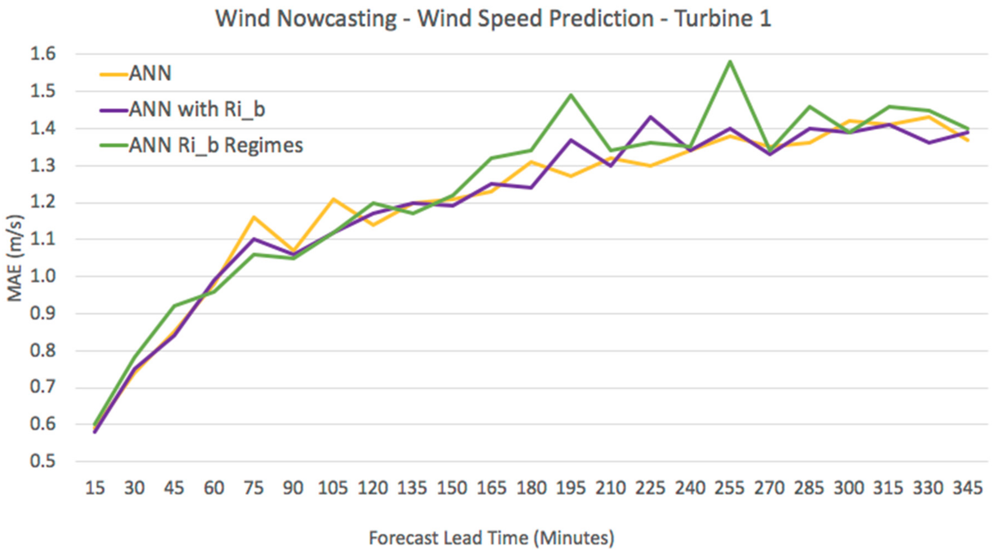
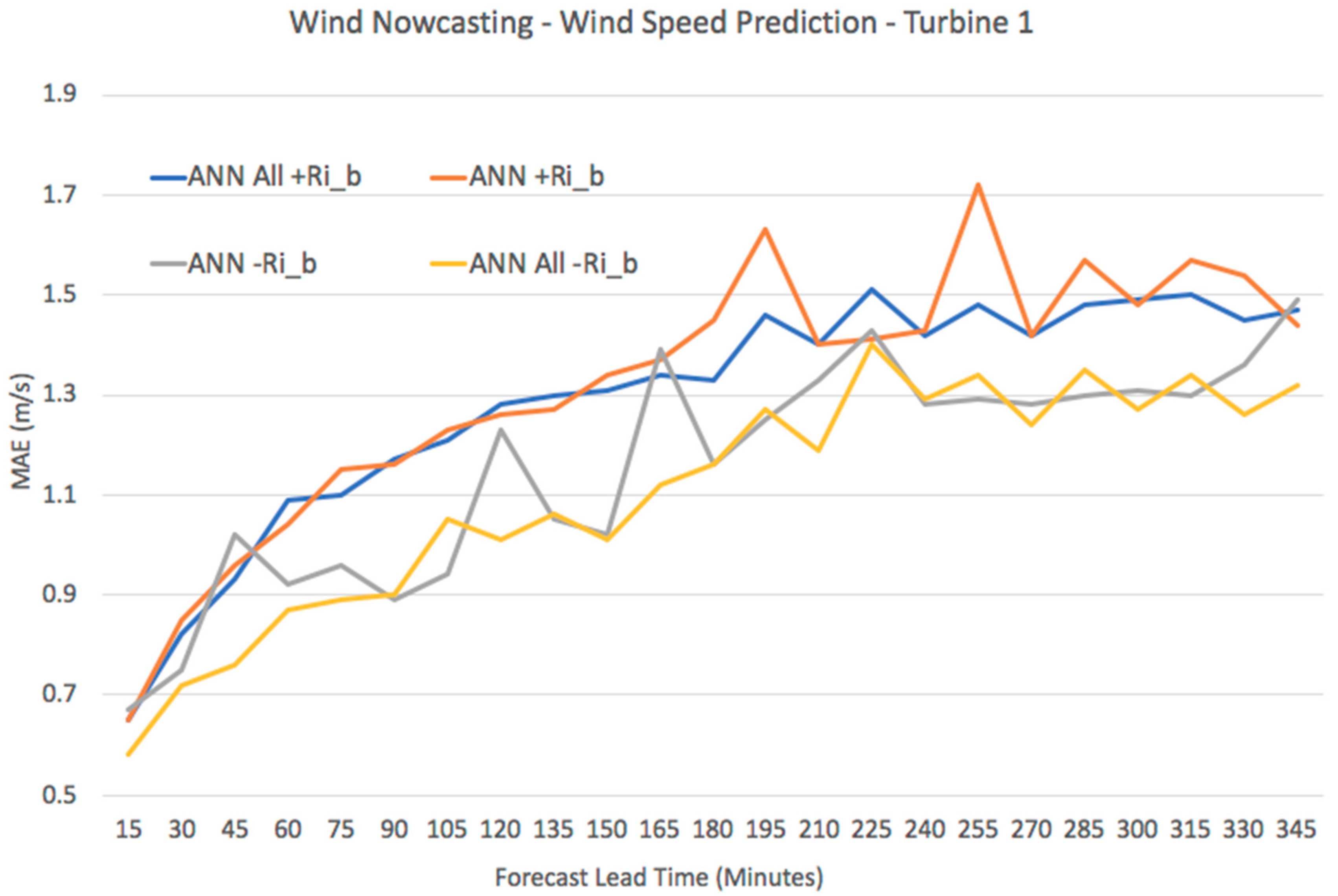
It is important to have high-quality short-range forecasts on the order of a few minutes out to about six hours to aid grid operators in maximizing wind and solar power utilization and minimizing associated costs in variable energy integration. To that end, KREPS includes AI-based “nowcasting” methods for both wind and solar as described in this section.

3.1. StatCast-Wind

The goal of the StatCast-Wind component of the prediction system is to improve wind speed prediction over DICast in the timeframe of 15 min to 6 h, utilizing machine learning with predictors including the DICast forecasts, surface observations, hour of the day, and month of the year.

3.1.1. StatCast-Wind Methodology

The wind energy climatology for the region near Shagaya [27] shows that the Shagaya plant experiences both diurnal and seasonal variability of hub-height wind speeds. The diurnal pattern of the wind speed tends to follow a pattern of lighter and more variable winds during the day, followed by an increase in wind speeds in the overnight hours, before decreasing around sunrise. Naegele et al. [27] indicates that this is likely due to the formation of a nocturnal low-level jet that produces stronger wind speeds in the evening and overnight hours. On the seasonal scale, the Asian monsoon has an impact on the region with Shamal winds producing strong, predominantly northwest wind during June, July, and August. The StatCast-Wind component attempts to improve upon what DICast is unable to capture in the physics of the predictability of the wind speed variability induced from the nocturnal low-level jets, Shamal wind patterns, and any synoptic or mesoscale weather phenomena. For the StatCast-Wind component, we test artificial neural networks (ANN) and random forest (RF) methods. Additionally, we assess utilizing stability information to build separate ANNs for unstable and stable regimes to better predict the evolution of the low-level nocturnal jet’s impact on hub-height wind speed.

3.1.2. StatCast-Wind Results

The StatCast-Wind machine learning methods were configured and tested over two years from 1 September 2017 through 31 August 2019. The initial step of the method assesses the impact of creating seasonal-based models on the system performance. The data were split into seasonal datasets for the Shamal wind dominated months (June, July, August) and non-Shamal wind dominated months. The baseline models were trained on the first year and tested on the second year. The seasonal models were trained on either the Shamal or non-Shamal seasonal datasets in the first year and applied to the respective Shamal or non-Shamal seasonal datasets for the second year. We conducted the test using both RFs and ANNs training on the entire year and for separate seasons. We found that there was no substantial difference for predictions of 15-min to 345-min forecast lead times between the seasonal models and the full-year model. As a result, we conclude that the underlying DICast model captures the Shamal wind synoptic-scale pattern that produces the typically higher wind speeds in the summer months.

Next, we tested the seasonal dependence of training the machine learning models and the stability-regime methodology for the non-Shamal season where the nocturnal low-level jets have more impact on the diurnal variability. Due to the availability of the Elecnor meteorological tower (the red star labeled ELE in Figure 2) observations necessary for computing the atmospheric stability in the boundary layer, we were limited to the period from 1 September 2017 through 27 February 2019. Therefore, we updated the training and test split to use the period from 1 September 2017 through 30 November 2018 as the training period and 1 December 2018 through 27 February 2019 as the testing period. The training period was further randomly split into 80% training and 20% validation to determine the optimal configurations of the machine learning models. A separate training and testing dataset were created for each forecast lead time, and individual models were trained for each forecast lead time independently. We removed any instance where there was a missing value in any of the predictors or predictand. Therefore, due to the amount of missing data for each of the observation stations, the final dataset consisted of a range of 5222 training instances and 1976 testing instances for the 15-min forecast lead time to 5007 training instances and 1974 testing instances for the 345-min forecast lead time. We present the results on the independent test dataset to quantify each model’s expected operational performance.

We used the bulk Richardson number (Ri_B) to identify whether the current state of the atmosphere is stable or unstable. Ri_B quantifies the ratio of buoyancy-driven turbulence to the shear-driven turbulence as described in [28]. The Ri_B calculation was performed using data from the nearby Elecnor meteorological tower (76-m anemometer and wind vane) and the surface weather stations (3 m for temperature and relative humidity and 4 m for wind speed and direction) in the PV farm. After the Ri_B was calculated for each 10-min interval to match the frequency of the observations, the datasets were merged with the DICast forecasts. Our initial test was to determine the sensitivity of the ANN to adding Ri_B as a predictor to the model or to separate the models by stability regime. We evaluated the performance of the methods compared to excluding Ri_B, and the results are displayed in Figure 7. On average, the ANN without regime separation or adding Ri_B as a predictor generally performs the best, but all methods perform similarly well. In the first hour of the model training the ANN separated by Ri_B tends to perform the worst, but transitions to performing slightly better during most of the second hour. After the second hour, the ANNs using stability regimes and the Ri_B as a predictor tends to have more variability in their predictions, which shows the sensitivity the ANN may have to small changes in stability; however, the errors tend to be worse, indicating that the stability models may be overfitting or over-emphasizing the effect of stability on wind speed evolution.

Next, we evaluated the error of the ANN and the stability regime ANNs when we separate the test dataset into unstable (-) and stable (+) regimes. The results on the test dataset are displayed in Figure 8, where the ANN “All” indicates the model was trained on all data and the errors are displayed in each regime, while the ANN +Ri_B indicates that the model was trained on the same (stable) stability regime as the test results. From this analysis, it is clear that the errors are higher in the unstable regime than the stable regime. Although the wind speed is typically higher at night when conditions are stable, it tends to be a less variable wind speed than during the day when conditions are unstable [27]. These results make physical sense as the model errors tend to be higher when there is higher variability (unstable) than in lower variability (stable) regimes. Generally, the ANN trained without regime identification displays less variability between forecast time periods, but the results on average are similar between the stability regime ANNs and the ANN trained on all data. One reason why the stability regime models may not show significant performance benefit is that by the time the final datasets were merged, there may not have been sufficient training cases to capture the full signal within the noise of the data. Another reason why the stability analysis may not show significant benefit is that the physics of the NWP underlying the DICast predictions as well as the nonlinear post-processing within the DICast integrator are adequately capturing the physics and the systematic error biases in each stability regime. If there were systematic errors in the different regimes, then the ANNs may capture those nonlinearities of the prediction problem, but there likely is not enough signal in the noise given the available data.

Finally, we evaluated DICast forecasts compared to machine learning techniques and a baseline of persistence and found that DICast and the RF performed the best overall. The results on the independent test dataset are shown in Figure 9 for forecast lead times of 15 min to 345 min ahead. All methods perform better than persistence (i.e., the wind speed remains steady at the current observation), which is not surprising given we would expect an NWP-based forecast to capture at least some of the physical evolution of the state of the atmosphere at Shagaya. It is also evident that the ANN performs worse than the RF and the DICast, which may indicate that the ANN tends to overfit the available training data. Although the RF and DICast perform similarly well, in the first hour (Figure 10), it is clear that the RF improves over DICast and may capture some of the non-linear relationships between the DICast forecast and the recent observations. Ultimately, the RF will be utilized for the first hour of predictions before transitioning to the DICast forecasts since the RF does not provide significant additional benefit after the first 60-min forecast lead time.

3.2. StatCast-Solar

The Shagaya PV farm is divided into two 5 MW sub-farms to evaluate the cost and performance of two different solar panel technologies (polycrystalline silicon and thin-film). All the panels in both PV farms are at a fixed tilt of 20°. PV panels use both direct and diffuse sunlight; therefore, an accurate prediction of GHI, a sum of the direct and diffuse radiation received on a horizontal plane at the earth’s surface, is critical in determining the energy generated from a PV farm. Both PV sub-farms at Shagaya include weather stations recording surface observations of wind speed and direction, relative humidity, temperature, panel temperature, GHI, and other meteorological variables. StatCast-Solar currently consists of a collection of AI models trained on surface observations from these weather stations, solar angles, and valid DICast forecast variables to make GHI predictions at 15-min intervals out to 345 min for each PV sub-farm.

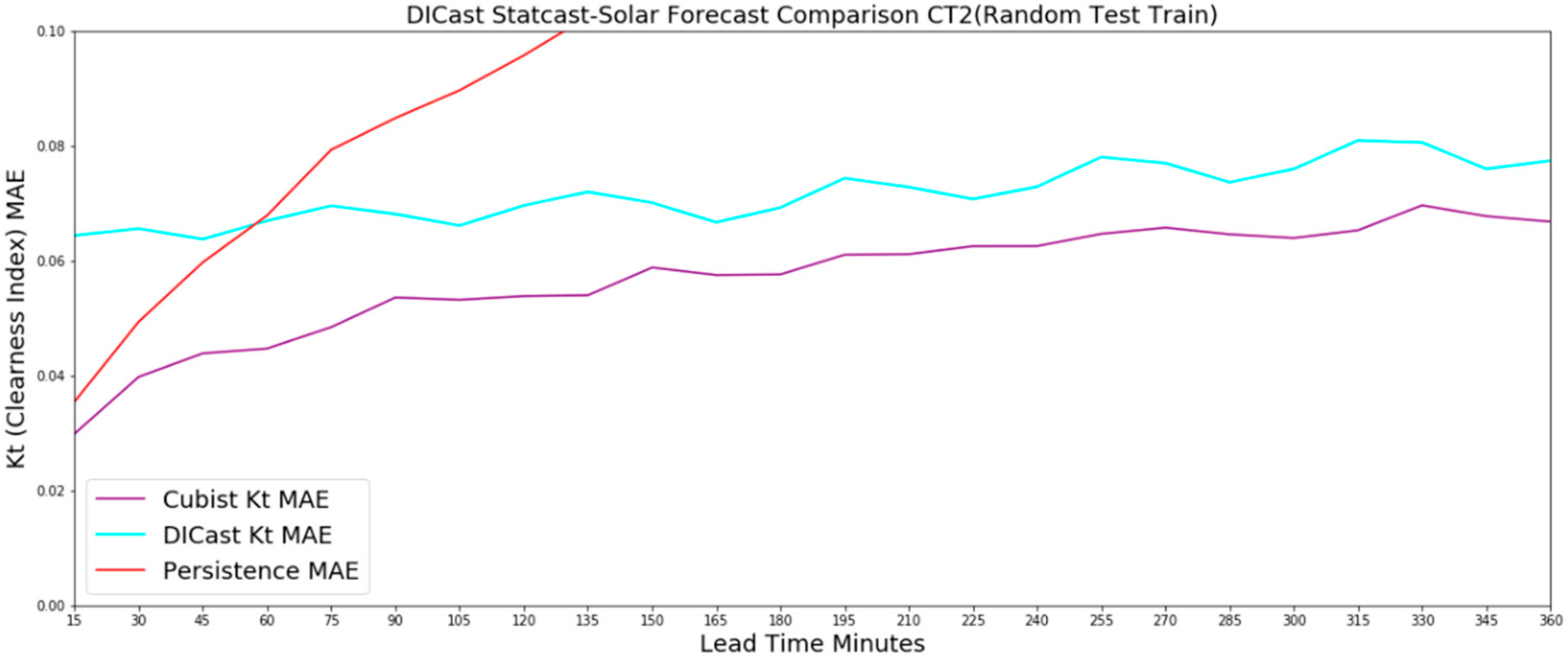
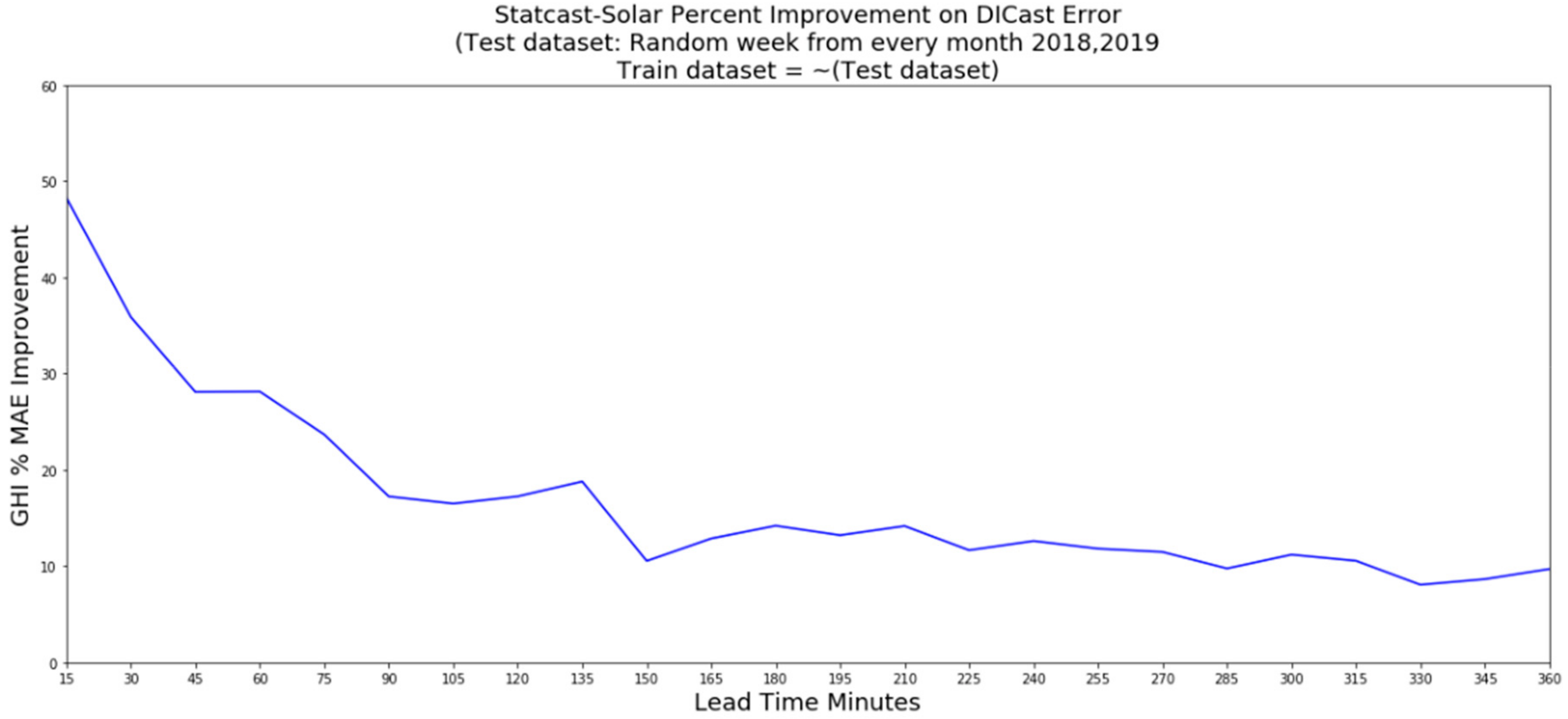
3.2.1. StatCast-Solar Methodology

The goal of StatCast-Solar is to make accurate short-range predictions of solar irradiance with machine learning algorithms. The predictand of the statistical learning models is the clearness index, Kt, which is the fraction of extraterrestrial radiation that reaches the earth’s surface after being scattered, reflected, and absorbed by the water droplets and ice crystals of clouds, air molecules, and aerosols. It is defined as the ratio of the GHI measured at the earth’s surface to the GHI at the top of the atmosphere. The clearness index is chosen over GHI as the predictand because it removes the diurnal and seasonal variations in GHI due to solar elevation cycles. Predictions of GHI are easily derived from predictions of Kt by multiplying by the appropriate value of the top of the atmosphere GHI (obtained by a model that is a function of date, time, and location).

To find the optimal machine learning algorithm for StatCast-Solar, we tested several supervised learning algorithms including RF, gradient boosted regression, ANN, and regression tree (Cubist) models. The models were trained and tested on data obtained from the Shagaya PV farm from September 2018–June 2019. The Cubist regression tree model had the best performance on the test dataset without overfitting the training dataset. The Cubist algorithm reduces the model tree, which has multivariate linear models at its nodes, into a set of understandable conditions and linear rules in which the predicted value is an average of values from all rules that apply to an input data sample. The algorithm makes an ensemble prediction and adds a boosting-like element by using a ‘committee’ scheme. A committee is formed by sequentially building model trees that adjust to errors in previous models, with the final prediction being an average of all of the predicted values of ‘members’ of the committee. For a detailed description of the Cubist algorithm see [29].

The following meteorological variables were available and considered as clearness index predictors: current observations of air temperature, Kt, meridional and zonal components of wind speed and direction, relative humidity, and average panel surface temperature; 90 minutes of historical averages of Kt over 15-min intervals; DICast value of cloud fraction at generation time; and valid DICast forecasts of Kt, air temperature, cloud cover, pressure, and dew point temperature. Different configurations of Cubist models were trained and tested for each forecast lead time from 15–345 minutes. Because ANN and cloud-based regime dependent ANNs (RD-ANN) performed successfully for Sacramento, California, USA [30,31], an in-depth comparison of ANN and Cubist regime-dependent and non-regime-dependent models was conducted to compare algorithm performance and to investigate the potential benefit of regime dependent models at the Shagaya PV farm. It was determined based on our testing and training data that Cubist models performed better than the ANN models and that there was no benefit to using regime-dependent models for this site with dominant clear sky conditions. Details of that analysis and results of experiments leading to that conclusion can be found in [32].

The following models were tested to determine the optimal model for each lead time:

• Cubist—Cubist models using only current observations of T, Kt, U, V, RH, and the previous 90-minute averages of Kt observations at 15-minute intervals plus valid DICast forecast variables of Kt, percent cloud cover, dew point, T, P.
• Kt Persistence—Clearness index remains constant between generation time and forecast time, also referred to as “smart” persistence because it allows the solar angle to change. This serves as a baseline.
• DICast—DICast forecast of Kt.

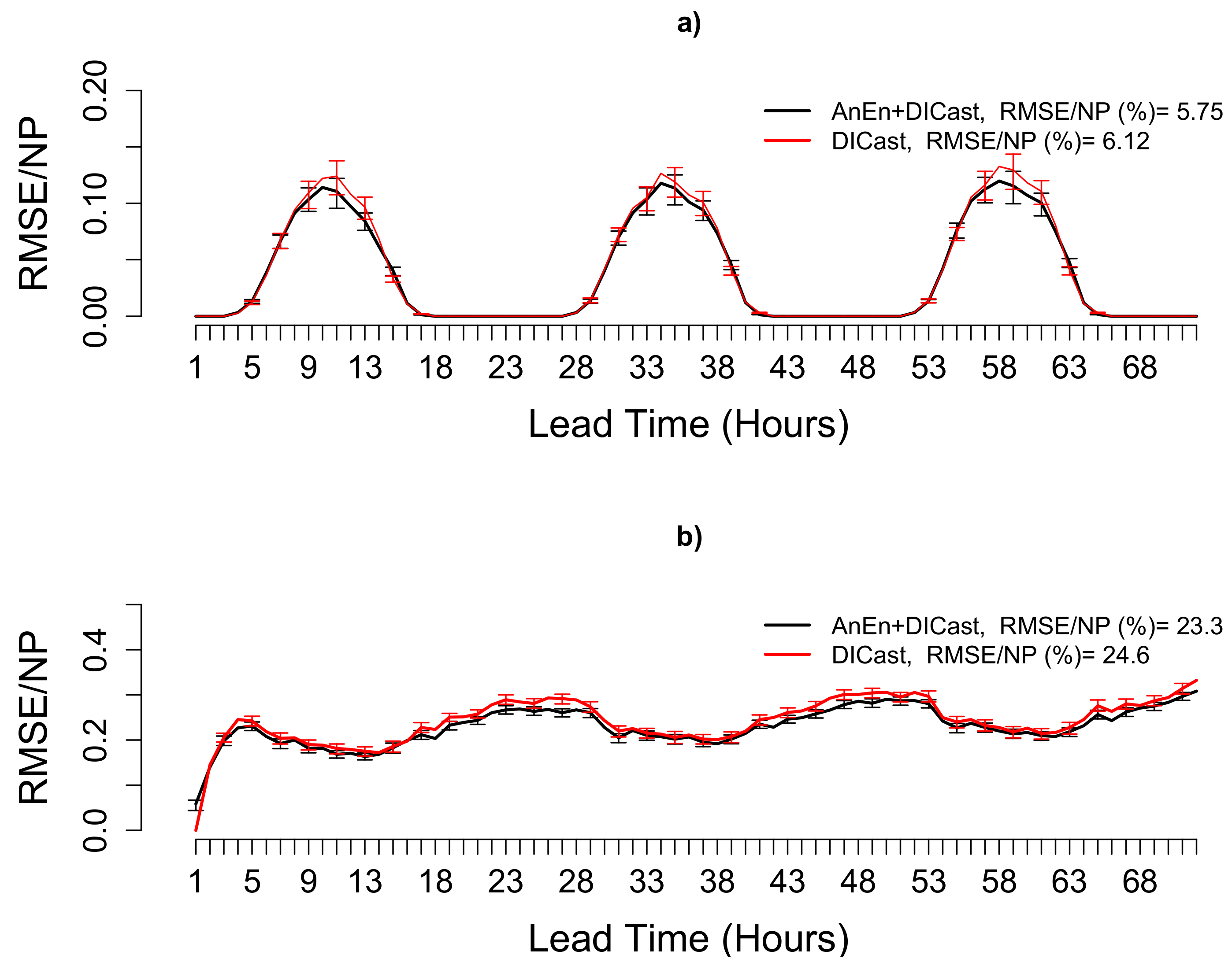
3.2.2. StatCast-Solar Results

The performance of the Cubist models can be seen in Figure 11 and Figure 12, which display mean absolute error (MAE) as a function of lead time. The Cubist-based models are superior to either smart persistence or the raw DICast forecast as seen in Figure 11. Figure 12 indicates the percentage improvement of StatCast-Solar over DICast in terms of MAE. We see improvements of nearly 50% at lead time 0 with decreases to about 10% beyond about 270 min.

4. Completing the Forecast

KREPS smartly blends the wind and solar forecasts from DICast, StatCast-Wind, and StatCast-Solar to produce a seamless forecast in time. A blended Nowcast forecast weights the nowcast components. Those weights vary with lead time and gradually weight DICast the highest to produce a smooth blend to the DICast forecast at the end of the 6-hour nowcast time period. The end-users, however, do not wish to focus on wind speed and GHI, but rather on power. Thus, KREPS includes the analog ensemble (AnEn) as a method to convert the meteorological variables to power as well as to quantify uncertainty as described in Section 4.1. In addition, users can leverage information on uncertainty in the predictions to better run reserve systems, prepare for large changes in the power output, and alleviate transmission bottlenecks [33,34,35]. The grid operators and KISR scientists need to be able to view the forecast, including the uncertainty quantification, in clear, actionable displays that are easy to read while providing the needed situational awareness. The displays are described in Section 4.2.

4.1. Analog Ensemble

To quantify uncertainty, the KREPS system uses the AnEn approach. These components include DICast^®, the AnEn, and the Schaake shuffle (SS) algorithm. DICast is used to build the archive of deterministic forecasts of the meteorological variables of interest, which are mainly hub-height wind speed and GHI. The AnEn takes the current meteorological DICast forecast as input and generates the wind and solar power ensemble predictions. The SS algorithm reorders the members to reestablish consistency across consecutive lead times and among production units.

4.1.1. AnEn Methodology

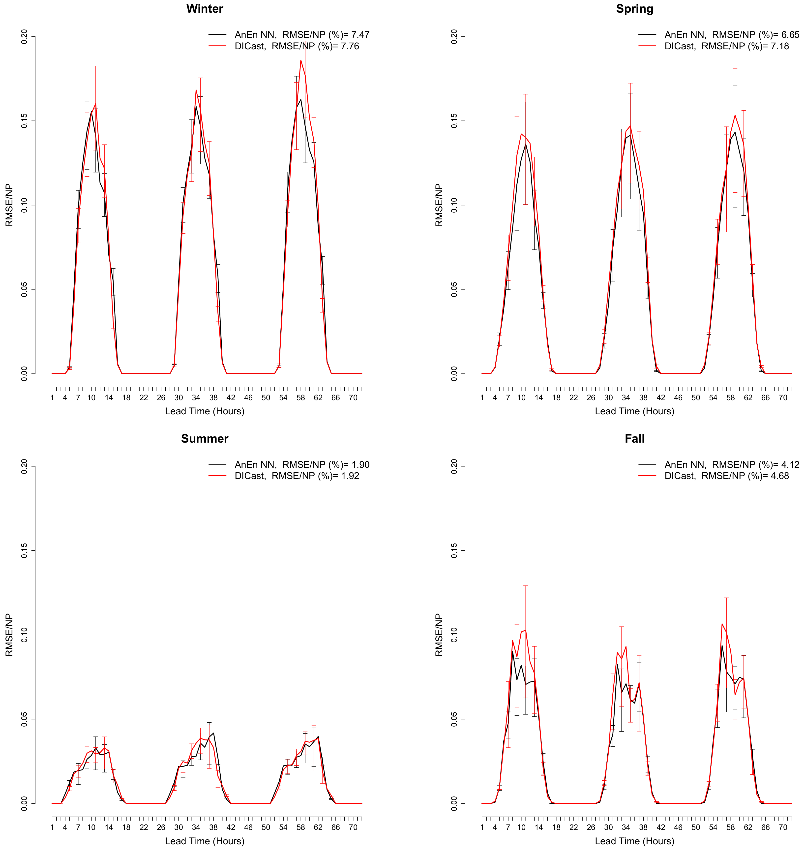
The AnEn technique has been widely used for renewable energy applications, among others, and is described in several works. Here we provide a brief description and refer the reader to [36,37,38] for more details. In this work, the AnEn is applied after the DICast^® post-processing of the meteorological variables (hereafter AnEn + DICast), which is similar to what was carried out in [39], where a neural network was used as a MOS [24] approach to improve the raw NWP deterministic output. For each lead time, and target forecast in the testing dataset, the AnEn set of power forecasts is constituted by 20 power observations in the training dataset, which are the ensemble members. These observations are those concurrent with the forecast at the same lead time, chosen across the training dataset based on their similarity to the target forecast. A Euclidean distance between the target and forecasts in the training dataset is used as a similarity criterion. Note that the AnEn does not employ a function (power conversion curve) to convert the meteorological quantities into power. In fact, the analog forecasts are selected using only meteorological predictors while the corresponding observed power values are compared directly with the ensemble power predictions. Wiener et al. [15] found that the AnEn performs at least as well as other potential power conversion algorithms.

The AnEn algorithm is applied independently for every forecast lead time and at each solar block and wind turbine. The order of the members is determined by the ranking of the Euclidean distance used as similarity criteria between the current forecast and the past analog forecasts. Hence, the first member in the ensemble is the past observation whose corresponding past forecast has the lowest distance while the 20th member is the one with the largest distance among the selected members. If this order is used to match the members across each wind or solar power site and at subsequent lead times, as demonstrated below, the resulting inter-production unit (PU) correlation structure from the ensemble members might not be the same as that of the observations. To overcome this limitation, the SS method [40] is applied to reorder the AnEn members as in previous work [41]. The application of the SS method to probabilistic power forecasts at Shagaya is described more fully in Alessandrini et al. [14]. In that work, the goal is to analyze the AnEn performance in terms of the spread/skill consistency of the ensemble predictions of total power obtained by adding the individual members from the individual wind and solar production units. A good correlation between the RMSE and spread (defined as the standard deviation about the ensemble mean) indicates that an ensemble system can predict its uncertainty [42] and ideally, the ensemble spread should match the RMSE at any lead time. In this paper instead, we limit our evaluation to the deterministic forecast obtained by taking the mean of the AnEn member at any lead time. We aim to further improve the DICast performance through the AnEn in terms of hourly wind and solar power prediction accuracy measured as RMSE.

4.1.2. AnEn Results

The dataset used to test our forecasting system consists of an archive from 1 September 2017 to 1 December 2019 of 0–72-h DICast forecasts. The solar application uses 1-h average GHI and cloud cover as meteorological predictors for the AnEn, along with power produced at the PV sub-farm, while the wind algorithm uses hub-height wind speed and direction, 2-m temperature, and the power observed at each wind turbine. Only forecasts initialized at 00 UTC are considered for this analysis, though the AnEn is run hourly in KREPS operationally. Data from 1 September 2017 to 31 August 2018 are used for training while data from 1 September 2018 to 1 December 2019 were used for testing. In Figure 13, the RMSE (solid lines) is plotted as a function of the forecast lead time for wind and solar power for both AnEn + DICast and DIcast. For both wind and solar power, AnEn + DICast exhibits slightly lower errors than DICast alone. The differences are more enhanced for wind power than solar power. In fact, the AnEn + DICast is statistically significantly better than DICast for a few lead times, as shown by the bootstrap intervals barely or not overlapping. At the first lead time, the DICast RMSE is 0 because the latest wind power observation is used as a forecast. On the other hand, the AnEn + DICast prediction at the first lead time is still made of an ensemble of past observations properly selected across the training dataset as explained earlier. The mean of this ensemble does not match the value of the latest wind power observation, which leads to an RMSE greater than 0.

Examining the RMSE values stratified by season (Figure 14 and Figure 15), winter and spring exhibit the worst performances for solar and wind power respectively, with the AnEn + DIcast generally still slightly overperforming compared to DICast alone. The performance is highly dependent on the season for solar power because of the climatology of Kuwait, with very frequent, easily predictable, clear sky conditions during the summer [43]. For wind power, there is an enhanced daily cycle in the RMSE in the summer with higher values during the night than during the day. This is explained by higher values of the wind speed during the night driven by the development of low-level jets as explained earlier in the paper and in [27]. Thus, we have demonstrated that the AnEn can be used to slightly improve upon the DICast deterministic forecast while additionally providing probabilistic information.

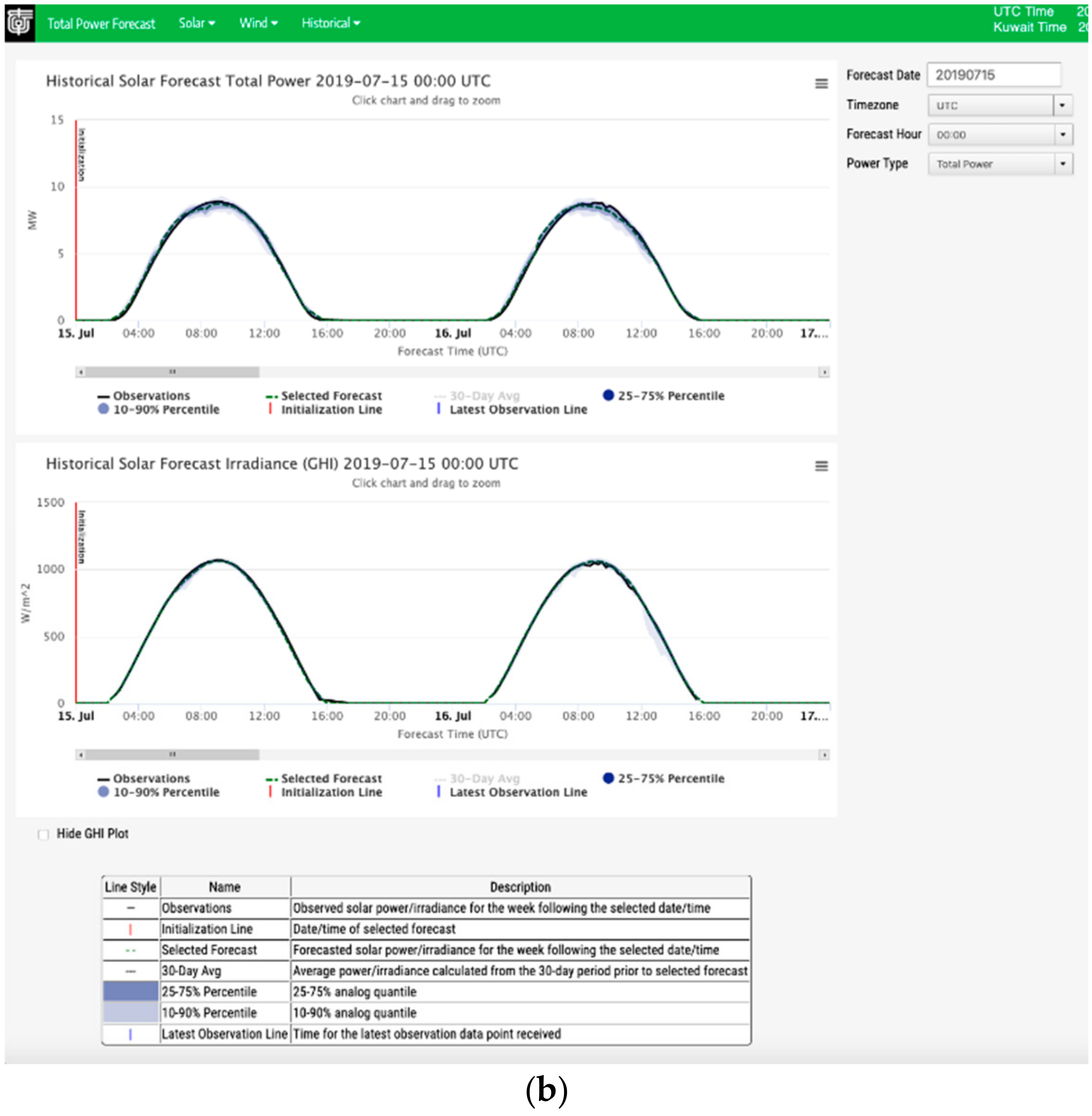
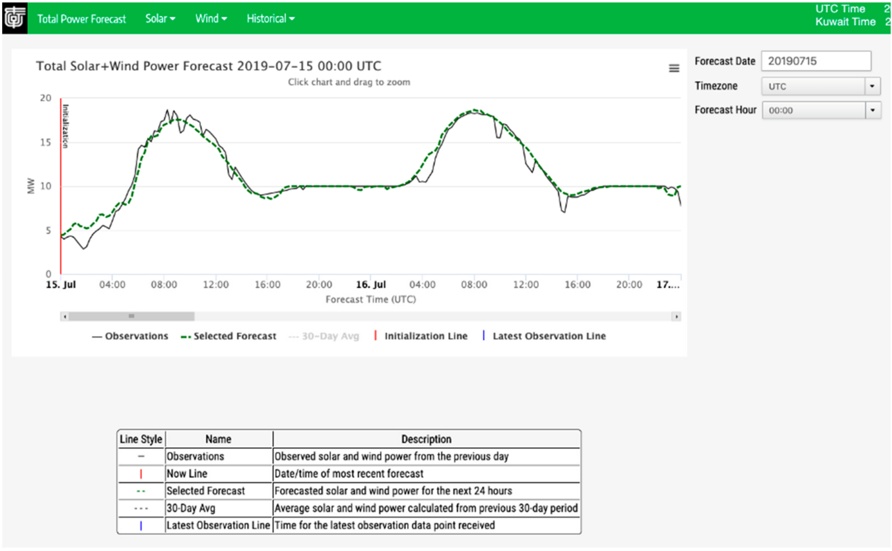
4.2. Viewing the Results

NCAR has developed web-based display technology as part of KREPS to allow grid operators and KISR personnel to interact with power forecast products, and to enable scientists to assess the performance of wind, solar, and total power predictions. The operator display is a three-tiered software application consisting of a database layer, RESTful web service layer, and web client as diagrammed in Figure 16.

This application is designed to provide decision support to end-users. It enables an interactive view into the forecast and observation time series and gives users the ability to zoom into specific sections of each series, scroll across dates and times, and toggle data series and error bars. The display plots the current wind and solar power forecasts, wind speed forecast, and GHI forecast, while blue-shaded quantile ranges based on the AnEn provide users an estimate of the forecast uncertainty (Figure 17). On the KREPS operator display, which was also designed to be colorblind-accessible, the forecasts (dashed green lines) are the AnEn mean, and, when available, observations are shown as solid black lines. When wind power observations are available, a solid purple line depicts the percentage of capacity available based on the operational status variable mentioned in Section 2.1.

Additionally, users can search for and view historical forecasts and their corresponding observations ingested from sensors at Shagaya as demonstrated in Figure 18. Using this feature, a retroactive assessment of forecast and observation data can be performed and general trends can be explored at specific forecast hours and times of the day.

The display also includes extreme event alerting capabilities for high wind speed and high temperatures that could cause wind turbine derating or cut-out. Additional techniques to infer the percent capacity of available wind turbines from sensor data are also being explored. There is a significant potential for the application of machine learning anomaly detection algorithms to assist with these problems and to monitor the state of the system while alerting display users to potential problems.

5. Conclusions

This paper describes a renewable power forecasting system that effectively blends physics-based forecasting with artificial intelligence methods. DICast directly bias corrects and optimizes blending coefficients to allow combining multiple NWP models in a forecast.

For nowcasting timeframes of less than about 6 hours, we saw that AI-based solar power forecasting methods are effective. Additionally, the AI-based wind power forecasting methods improve on the DICast forecast for the first hour for wind and beyond for solar.

The Analog Ensemble method provides well-calibrated probabilistic forecasts while converting to power. Note that in prior versions of the NCAR system [44], the AnEn corrected the wind speed or irradiance forecast, then a separate power conversion algorithm provided the power forecast. For KREPS, however, the AnEn is quite competitive with other power conversion algorithms [15] so it is directly trained to produce power forecasts. In addition, this is the first time that the uncertainty of wind and solar power forecasts are combined using a Schaake shuffle AnEn technique [14].

KREPS has demonstrated that improvements occur when AI is used both to correct and supplement the physically-based forecasting systems. Total error is decreased when AI methods are employed. It also allows smooth forecast blending across scales, where the nowcast which improves upon DICast, blend, and transitions into a smooth forecast. The probabilistic forecasts are displayed to the end-user to provide actionable decision support.

Future work will explore using these techniques in other climate regimes and emphasize fully gridded forecasting methods, particularly in locales where distributed variable generation is prevalent. In addition, NCAR is exploring forecasting for situations where storage is available and decisions must be made for when to charge and discharge the batteries. Such advances in forecasting for the variable renewables are becoming more necessary as the penetration of renewables is increasing. Thus, continued advances in forecasting methods are becoming more important to facilitate the transition to a renewable-based energy system that is reliable, economical, and efficient.

References

1. IEA. Renewables 2018: Market Analysis and Forecast from 2018 to 2023; International Energy Agency: Paris, France, 2018; Available online: https://www.iea.org/renewables2018 (accessed on 8 October 2019).
2. Xcel Energy. A Carbon-Free Future. Xcel Energy Corporate Responsibility Report. 2019. Available online: https://www.xcelenergy.com/company/corporate_responsibility_report/library_of_report_briefs/a_carbon_free_future (accessed on 8 October 2019).
3. Inman, R.H.; Pedro, H.T.C.; Coimbra, C.F.M. Solar forecasting methods for renewable energy integration. Prog. Energy Combust. Sci. 2013, 39, 535–576. [Google Scholar] [CrossRef]
4. Tuohy, A.; Zack, J.; Haupt, S.E.; Sharp, J.; Ahlstrom, M.; Dise, S.; Grimit, E.; Möhrlen, C.; Lange, M.; Garcia Casado, M.; et al. Solar forecasting: Methods, challenges, and performance. IEEE Power Energy Mag. 2015, 13, 50–59. [Google Scholar] [CrossRef]
5. Giebel, G.; Kariniotakis, G. Wind power forecasting—A review of the state of the art. In Renewable Energy Forecasting: From Models to Applications; Kariniotakis, G., Ed.; Woodhead Publishing: Cambridge, MA, USA, 2017; 373p. [Google Scholar] [CrossRef]
6. Orwig, K.D.; Ahlstrom, M.; Banunarayanan, V.; Sharp, J.; Wilczak, J.M.; Freedman, J.; Haupt, S.E.; Cline, J.; Bartholomie, O.; Hamman, H.; et al. Recent trends in variable generation forecasting and its value to the power system. IEEE Trans. Renew. Energy 2014, 6, 924–933. [Google Scholar] [CrossRef]
7. Haupt, S.E. Short-range forecasting for energy. In Weather & Climate Services for the Energy Industry; Troccoli, A., Ed.; Palgrave Macmillan: Cham, Switzerland, 2018; 197p. [Google Scholar] [CrossRef] [Green Version]
8. Mahoney, W.P.; Parks, K.; Wiener, G.; Liu, Y.; Myers, W.L.; Sun, J.; Delle Monache, L.; Hopson, T.; Johnson, D.; Haupt, S.E. A wind power forecasting system to optimize grid integration. IEEE Trans. Sustain. Energy 2012, 3, 670–682. [Google Scholar] [CrossRef]
9. Haupt, S.E.; Kosović, B.; Jensen, T.; Lazo, J.K.; Lee, J.A.; Jiménez, P.A.; Cowie, J.; Wiener, G.; McCandless, T.C.; Rogers, M.; et al. Building the Sun4Cast system: Improvements in solar power forecasting. Bull. Am. Meteor. Soc. 2018, 99, 121–136. [Google Scholar] [CrossRef]
10. KISR. 2019 Kuwait Energy Outlook: Sustaining Prosperity through Strategic Energy Management; Kuwait Institute for Scientific Research: Shuwaikh, Kuwait, 2019; 84p, Available online: https://www.arabstates.undp.org/content/dam/rbas/doc/Energy%20and%20Environment/KEO_report_English.pdf (accessed on 8 October 2019).
11. Al-Rasheedi, M.; Gueymard, C.A.; Al-Khayat, M.; Ismail, A.; Lee, J.A.; Al-Duaj, H. Performance evaluation of a utility-scale dual-technology photovoltaic power plant at the Shagaya Renewable Energy Park in Kuwait. Renew. Sustain. Energy Rev. 2020. submitted. [Google Scholar]
12. Warner, T.T. Numerical Weather and Climate Prediction; Cambridge University Press: New York, NY, USA, 2011; 526p, ISBN 978-0-521-51389-0. [Google Scholar]
13. Jiménez, P.A.; Lee, J.A.; Kosović, B.; Haupt, S.E. Solar resource evaluation with numerical weather prediction models. In Solar Resources Mapping: Fundamentals and Applications; Polo, J., Sanfilippo, A., Pomares, L., Eds.; Green Energy and Technology; Springer Nature: Cham, Switzerland, 2019; 367p. [Google Scholar] [CrossRef]
14. Alessandrini, S.; McCandless, T.C. The Schaake shuffle technique to combine solar and wind power probabilistic forecasting. Energies 2020. submitted for publication. [Google Scholar]
15. Wiener, G.; Brummet, T.; Linden, S.; Pearson, J.; Srivastava, I.; Alessandrini, S.; Al-Rasheedi, M. An evaluation of wind and solar power conversion methods. Energies 2020. submitted for publication. [Google Scholar]
16. Myers, W.; Wiener, G.; Linden, S.; Haupt, S.E. A consensus forecasting approach for improved turbine hub height wind speed predictions. In Proceedings of the AWEA Windpower Conference & Exhibition, Anaheim, CA, USA, 24 May 2011. [Google Scholar]
17. Powers, J.G.; Klemp, J.B.; Skamarock, W.C.; Davis, C.A.; Dudhia, J.; Gill, D.O.; Coen, J.L.; Gochis, D.J.; Ahmadov, R.; Peckham, S.E.; et al. The Weather Research and Forecasting model: Overview, system efforts, and future directions. Bull. Am. Meteor. Soc. 2017, 98, 1717–1737. [Google Scholar] [CrossRef]
18. Jiménez, P.A.; Hacker, J.P.; Dudhia, J.; Haupt, S.E.; Ruiz-Arias, J.A.; Gueymard, C.A.; Thompson, G.; Eidhammer, T.; Deng, A. WRF-Solar: An augmented NWP model for solar power prediction. Bull. Am. Meteor. Soc. 2016, 97, 1249–1264. [Google Scholar] [CrossRef]
19. Jiménez, P.A.; Alessandrini, S.; Haupt, S.E.; Deng, A.; Kosović, B.; Lee, J.A.; Delle Monache, L. The role of unresolved clouds on short-range global horizontal irradiance predictability. Mon. Weather Rev. 2016, 144, 3099–3107. [Google Scholar] [CrossRef]
20. Tallapragada, V.; Manikin, G. Implementation of NGGPS/FV3GFS V1.0: GDAS/GFS V15.0.0 for Q2FY2019. NCEP OD Science and Decisional Brief; 1 October 2018. Available online: http://www.emc.ncep.noaa.gov/users/Alicia.Bentley/fv3gfs/updates/OD_Brief_10-01-18_FV3GFS.pptx (accessed on 29 January 2020).
21. Manikin, G.; Bentley, A.; Dawson, L.; Dorian, T. The Implementation of GFSv15. NCEP/EMC Model Evaluation Group; 13 June 2019. Available online: http://www.emc.ncep.noaa.gov/users/Alicia.Bentley/fv3gfs/updates/MEG_6-13-19_GFSv15.pptx (accessed on 29 January 2020).
22. Husain, S.Z.; Girard, C.; Qaddouri, A.; Plante, A. A new dynamical core of the Global Environmental Multiscale (GEM) model with a height-based terrain-following vertical coordinate. Mon. Weather Rev. 2019, 147, 2555–2578. [Google Scholar] [CrossRef] [Green Version]
23. McTaggart-Cowan, R.; Vaillancourt, P.A.; Zadra, A.; Chamberland, S.; Charron, M.; Corvec, S.; Milbrandt, J.A.; Paquin-Ricard, D.; Patoine, A.; Roch, M.; et al. Modernization of atmospheric physics parameterization in Canadian NWP. J. Adv. Model. Earth Syst. 2019, 11, 3593–3635. [Google Scholar] [CrossRef] [Green Version]
24. Glahn, H.R.; Lowry, D.A. The use of Model Output Statistics (MOS) in objective weather forecasting. J. Appl. Meteorol. 1972, 11, 1203–1211. [Google Scholar] [CrossRef] [Green Version]
25. Haupt, S.E.; Kosović, B. Variable generation power forecasting as a big data problem. IEEE Trans. Sustain. Energy 2017, 8, 725–732. [Google Scholar] [CrossRef]
26. Myers, W.; Chen, F.; Block, J.; Burnsville, M.N. Application of atmospheric and land data assimilation systems to an agricultural decision support system. In Proceedings of the 28th Conference on Agricultural and Forest Meteorology, American Meteorological Society, Orlando, FL, USA, 27 April–2 May 2008; Available online: http://ams.confex.com/ams/28Hurricanes/techprogram/paper_138947.htm (accessed on 10 February 2020).
27. Naegele, S.M.; McCandless, T.C.; Greybush, S.J.; Young, G.S.; Haupt, S.E.; Al-Rasheedi, M. Climatology of wind variability for the Kuwait region. Renew. Sustain. Energy Rev. 2020. conditionally accepted and in revision. [Google Scholar]
28. Stull, R.B. An Introduction to Boundary Layer Meteorology; Kluwer Academic Publishers: Boston, MA, USA, 1988; 666p. [Google Scholar] [CrossRef]
29. Quinlan, J.R. Learning with continuous classes. In Proceedings of the Australian Joint Conference on AI, Hobart, Australia, 16–18 May 1992; pp. 343–348. [Google Scholar]
30. McCandless, T.C.; Young, G.S.; Haupt, S.E.; Hinkelman, L.M. Regime-dependent short-range solar irradiance forecasting. J. Appl. Meteorol. Climatol. 2016, 55, 1599–1613. [Google Scholar] [CrossRef]
31. McCandless, T.C.; Haupt, S.E.; Young, G.S. A regime-dependent artificial neural network technique for short-range solar irradiance forecasting. Renew. Energy 2016, 89, 351–359. [Google Scholar] [CrossRef] [Green Version]
32. McCandless, T.C.; Dettling, S.; Haupt, S.E. Comparison of implicit vs. explicit regime identification in machine learning methods for solar irradiance prediction. Energies 2020, 13, 689. [Google Scholar] [CrossRef] [Green Version]
33. Dobschinski, J.; Bessa, R.; Du, P.; Geisler, K.; Haupt, S.E.; Lange, M.; Möhrlen, C.; Nakafuji, D.; de la Torre Rodriguez, M. Uncertainty forecasting in a nutshell. IEEE Power Eng. Syst. 2017, 15, 40–49. [Google Scholar] [CrossRef] [Green Version]
34. Bessa, R.J.; Möhrlen, C.; Fundel, V.; Siefert, M.; Browell, J.; Haglund El Gaidi, S.; Hodge, B.-M.; Cali, U.; Kariniotakis, G. Towards improved understanding of the applicability of uncertainty forecasts in the electric power industry. Energies 2017, 10, 1402. [Google Scholar] [CrossRef]
35. Haupt, S.E.; Garcia Casado, M.; Davidson, M.; Dobschinski, J.; Du, P.; Lange, M.; Miller, T.; Möhrlen, C.; Motley, A.; Pestana, R.; et al. The use of probabilistic forecasts: Applying them in theory and practice. IEEE Power Energy Mag. 2019, 17, 46–57. [Google Scholar] [CrossRef]
36. Alessandrini, S.; Delle Monache, L.; Sperati, S.; Nissen, J. A novel application of an analog ensemble for short-term wind power forecasting. Renew. Energy 2015, 76, 768–781. [Google Scholar] [CrossRef]
37. Alessandrini, S.; Delle Monache, L.; Sperati, S.; Cervone, G. An analog ensemble for short-term probabilistic solar power forecast. Appl. Energy 2015, 157, 95–110. [Google Scholar] [CrossRef] [Green Version]
38. Delle Monache, L.; Eckel, F.A.; Rife, D.L.; Nagarajan, B.; Searight, K. Probabilistic weather prediction with an analog ensemble. Mon. Weather Rev. 2013, 141, 3498–3516. [Google Scholar] [CrossRef] [Green Version]
39. Cervone, G.; Clemente-Harding, L.; Alessandrini, S.; Delle Monache, L. Short-term photovoltaic power forecasting using Artificial Neural Networks and an Analog Ensemble. Renew. Energy 2017, 108, 274–286. [Google Scholar] [CrossRef] [Green Version]
40. Clark, M.; Gangopadhyay, S.; Hay, L.; Rajagopalan, B.; Wilby, R. The Schaake shuffle: A method for reconstructing space–time variability in forecasted precipitation and temperature fields. J. Hydrometeorol. 2004, 5, 243–262. [Google Scholar] [CrossRef] [Green Version]
41. Sperati, S.; Alessandrini, S.; Delle Monache, L. Gridded probabilistic weather forecasts with an analog ensemble. Q. J. R. Meteor. Soc. 2017, 143, 2874–2885. [Google Scholar] [CrossRef]
42. Hopson, T.M. Assessing the ensemble spread-error relationship. Mon. Weather Rev. 2014, 142, 1125–1142. [Google Scholar] [CrossRef]
43. Tye, M.R.; Haupt, S.E.; Gilleland, E.; Kalb, C.; Jensen, T. Assessing evidence for weather regimes governing solar power generation in Kuwait. Energies 2019, 12, 4409. [Google Scholar] [CrossRef] [Green Version]
44. Kosović, B.; Haupt, S.E.; Adriaansen, D.; Alessandrini, S.; Wiener, G.; Delle Monache, L.; Liu, Y.; Linden, S.; Jensen, T.; Cheng, W.; et al. A comprehensive wind power forecasting system integrating artificial intelligence and numerical weather prediction. Energies 2020, 13, 1372. [Google Scholar] [CrossRef] [Green Version]
Figure 1. Map of Kuwait (yellow outline), with the Shagaya Renewable EnergyPark boundary (black polygon) in western Kuwait.
Energies 13 01979 g001
Figure 2. Map of Shagaya Renewable Energy Park Phase 1 installations, with Phase 1 & 2 boundary fence (black polygon), 10-MW wind plant (turbine icons), 10-MW PV plant (green rectangle), 50-MW CSP plant (blue rectangle), weather stations (yellow diamonds), and met towers (red stars).
Energies 13 01979 g002
Figure 3. Diagram of components of KREPS. AI-based forecasting components are colored orange and gold.
Energies 13 01979 g003
Figure 4. A schematic view of DICast®.
Energies 13 01979 g004
Figure 5. Average root mean square error (RMSE) of hub-height wind speed over the period 1 December 2018 to 30 November 2019 for forecasts valid at 06 UTC.
Energies 13 01979 g005
Figure 6. Average RMSE of global horizonal irradiance (GHI) over the period 1 December 2018 to 30 November 2019 for forecasts valid at 06 UTC.
Energies 13 01979 g006
Figure 7. Results (MAE) for the artificial neural networks (ANN) (gold line) compared to stability-regime dependent ANNs separated by unstable (−) and stable (+) regimes (green line) compared to the ANNs trained with bulk Richardson number (RiB) as a predictor (purple line).
Energies 13 01979 g007
Figure 8. Results (MAE) for the ANN trained on all data and applied to each stability regime separately compared to the stability-regime dependent ANNs separated by unstable (−) and stable (+) regimes and applied to the same stability regime as the one trained on.
Energies 13 01979 g008
Figure 9. Results (MAE) for the random forest (blue line), ANN (gold line), persistence (orange line), and the DICast hub height wind speed forecast (gray line) that show the DICast and RF perform similarly well.
Energies 13 01979 g009
Figure 10. Results (MAE)for the random forest (blue line), ANN (gold line), persistence (orange line), and the DICast hub height wind speed forecast (gray line) in the first 60 min show that the RF improves upon DICast for the first hour and the ANN improves upon DICast for the first 45 minutes.
Energies 13 01979 g010
Figure 11. Results for the Cubist model configurations compared to the DICast forecasts of Kt and smart persistence. The Cubist-based method performs best for all time periods from 15 min to 360 min compared to either DICast or smart persistence.
Energies 13 01979 g011
Figure 12. Percentage improvement of StatCast-Solar over DICast for all lead times from 15 min to 360 min.
Energies 13 01979 g012
Figure 13. Root mean squared error for AnEn + DICast (black) and DICast (red) for solar power (a) and wind power (b). The vertical bars represent the 5%–95% bootstrap intervals that are plotted every other lead time to reduce clutter. RMSE values are normalized by the nominal power of a single turbine (2 MW) or of a single PV plant (5 MW) and they are obtained by pooling data from all wind turbines or solar plants together. The values in the legends are obtained by averaging over the lead times and are shown as a percentage.
Energies 13 01979 g013
Figure 14. As Figure 13, but for solar power only with data stratified by season.
Energies 13 01979 g014
Figure 15. As Figure 13, but for wind power only with data stratified by season.
Energies 13 01979 g015
Figure 16. The architecture of the KREPS display.
Energies 13 01979 g016
Figure 17. Example forecasts (dashed green lines) and observations (solid black lines) for (a) wind and (b) solar power for the KREPS forecast issued on 15 Jul 2019 at 00 UTC.
Energies 13 01979 g017aEnergies 13 01979 g017b
Figure 18. Historical total power forecast issued on 15 Jul 2019 at 00 UTC.
Energies 13 01979 g018