Fuzzy Control of Waves Generation in a Towing Tank


1
Department of Electric Drives and Energy Conversion, Faculty of Electrical and Control Engineering, Gdańsk University of Technology, Narutowicza 11/12, 80-233 Gdańsk, Poland
2
Maritime Advanced Research Centre (CTO S.A.), Szczecińska 65, 80-392 Gdańsk, Poland
*
Author to whom correspondence should be addressed.
Energies 2020, 13(8), 2049; https://doi.org/10.3390/en13082049
Submission received: 6 March 2020
/
Revised: 2 April 2020
/
Accepted: 11 April 2020
/
Published: 20 April 2020
(This article belongs to the Special Issue Control Strategies for Power Conversion Systems)
Abstract
:This paper presents the results of research related to the transformation of electrical energy into potential and kinetic energy of waves generated on the water surface. The waves are generated to model the environmental conditions for the needs of the model tests. The model tests are performed on model-scale objects to predict the features of full-scale maritime objects. It is done to improve human safety and the survivability of constructions. Electrical energy is transformed into the energy of the water waves using a wave maker. The wave maker considered is a facility with an electrohydraulic drive and an actuator submerged into the water. The actuator movement results in the waves being mechanically-generated in accordance with the wave maker theory. The study aimed to investigate the advantage of the newly implemented fuzzy-logic controller over the hitherto cascading proportional-integral controllers of the wave maker actuator. The research was focused on experimental investigation of the transformation process outcomes harvested under the fuzzy-logic controller, versus the cascading proportional-integral controllers. The waves were generated and measured in the real towing tank, located in the Maritime Advanced Research Centre (CTO S.A.). The investigation confirmed the advantage of the fuzzy-logic controller. It provides more accurate transformation of energy into the desired form of the water waves of specified parameters—frequency and amplitude—and more flat amplitude-frequency characteristic of the transformation process.
1. Introduction
Physical model tests are of paramount importance for improving the safety of maritime structures. The model tests, carried out on the reduced-scale models (Figure 1), allow the prediction of the properties of full-scale objects, such as ships, oil rigs, wind turbines or wave energy converters, in their environment conditions [1]. The full-scale prediction, based on the reduced-scale model tests, is justified under the similitude, pursuant to the Buckingham theorem [2]. This kind of model test is performed in hydromechanics laboratories worldwide [3,4,5,6]. It finally improves the maritime safety and survivability of naval, offshore and onshore constructions as well as improving their performance.
The proper realization of the model tests requires accurate modelling of the environmental conditions in the scope of waves. The waves are modelled to reflect the conditions of the target type of sea and state of the sea on the model-scale, with the use of a wave maker [8]. The wave maker is a facility intended for transformation of the energy into the desired form of water waves. The facility consists of the actuator submerged into the water and the drive. The actuator oscillates into the water and mechanically generates the waves in accordance with a transfer function derived from wave maker theory and specific to geometry of the actuator.
The wave maker theory was early formulated by Havelock in 1929 [9]. Afterwards, the formulas called Biésel Transfer Functions, were derived by Biésel and Suquet in 1951 [10,11,12,13]. These works relate to the linear wave maker theory, that links the movements of the wave maker actuator with the profile of the generated wave. The experimental research carried out in the hydromechanics laboratories, validated the linear wave maker theory as sustainable within the waves of low steepness [14,15,16,17]. For the waves of high steepness, the nonlinearities and energy losses appear, making the linear theory inapplicable [17]. The development of weakly-nonlinear wave maker theories, allowed to extend the range of the theoretically covered physics, related to wave generation processes in typical wave flumes [18,19,20,21,22]. The more advanced techniques were also considered to simulate the generation of nonlinear waves numerically [23,24,25,26,27,28,29,30,31,32,33]. The complete nonlinear theory of the wave maker for the physical towing tank, up to now, is being developed and improved [34,35,36]. Thus, the linear wave maker theory, is validated to link the movements of the wave maker actuator with the profile of the low steepness waves, generated in the real towing tank. This is covered by the general formulation (1), where is the wave amplitude, is a wave maker stroke, h is a level of the waterplane above the bottom and k is a wave number [10,11,12,13].
The wave maker of a flap-type actuator with an electrohydraulic or electric drive is broadly applied [37]. This type of the facility was made available for the research in the deepwater towing tank by the Maritime Advanced Research Centre (CTO S.A.). The wave maker considered, is presented in Figure 2.
On the basis of the transfer function derived, for the geometry of the flap-type wave maker [34], the is associated with the amplitude of the wave maker flap oscillations at the waterplane a as follows (2).
is a constant coefficient, specific for the facility considered, and is equal to 0.8 [34]. It reflects the efficiency of the mechanical energy transformation into the form of the progressive sinusoidal waves due to the pressure loss in the water gap between the walls of the towing tank and the flap of the wave maker. is the level of the hinge above the bottom. k is associated with the harmonic frequency via the dispersion relation (3).
The previous control system of the wave maker considered, was composed of two obsolete cascading proportional–integral–derivative PID controllers, designed in the 1970s. The first one controlled the wave maker flap velocity in the inner loop. The second one controlled the wave maker flap position in the outer loop. The control algorithm was applied using an operational amplifiers and capacitors [38]. It was modernized by translation the original control algorithm into a digital form using an 8-bit AVR microcontroller [39,40]. Subsequently, it was tuned with the Åström-Hägglund relay method [41]. Afterwards, the control algorithm was successfully developed into the form of two cascading PI controllers, properly tuned and implemented with a 32-bit Advanced RISC Machine ARM microcontroller [7]. Despite the stability and fine quality of regulation of the implemented control system, there was still room for improvement. The amplitude-frequency characteristic, experimentally determined for the proportional–integral controllers PIs-based system, was not flat enough within the operating frequencies [7]. It induced unfavourable dependence of generated wave amplitude on its frequency. This disadvantage was manifested by a decrease of the wave amplitude whilst the desired wave frequency increased. It was hindering the model tests significantly. However, fuzzy-logic controller of Mamdani-type was successfully applied versus PI and PID controllers to achieve higher performance of electrohydraulic actuators in other applications [42,43,44]. The greatly satisfactory results reported there allowed us to expect improvement of the wave maker performance for the control system based on the fuzzy-logic controller, versus the hitherto applied cascading PI ones.
The objectives and scope of the research aimed to investigate the flatness improvement of the amplitude-frequency characteristics for waves generation process with use of the one fuzzy-logic controller (FL), versus the cascading PIs. The FL was expected to improve the performance of the energy transformation process and obtain a much more flat amplitude-frequency characteristic to provide more accurate control over the process of modeling the environmental conditions.
2. Energy Transformation
The energy , related to progressive sinusoidal wave on the water surface, includes the potential energy and kinetic energy . It is given by the formula (4), that expresses amount of the energy per unit of the water surface [1].
The is the water density. The g is the standard acceleration due to gravity. The is the amplitude of progressive sinusoidal wave of the frequency f. The two-dimensional progressive sinusoidal wave on the water surface is graphically depicted in Figure 3.
The time domain model of the water waves that occur in the environment can be considered a summation of two-dimensional progressive sinusoidal waves, derived in the form of (5) [8].
The and are the amplitude and frequency of the subsequent components—sinusoidal progressive waves. The is the random phase distributed in the range of 0 to and applied due to the space-time randomness of the process in the environmental conditions, related to waves. The summation of two-dimensional progressive sinusoidal waves in accordance with (5) is graphically depicted in Figure 4.
Therefore, the energy E, expressed per unit of the water surface and related to the water waves considered as (5), is derived as (6).
The time domain mathematical model of the subsequent progressive sinusoidal waves can be transformed to the frequency domain into the form of harmonics of the amplitudes at the frequencies of . Consequently, the waves on the water surface can be formulated in the form of the energy spectral density harmonics , as follows (7) [45].
A and B are the parameters that can be specified depending on the modelled type of sea [45] and the modelled state of the sea [46].
Accordingly, the energy expressed per unit of the water surface and related to the harmonic of the energy spectral density (7) is derived as (8).
The energy of the wind waves, naturally occurring in the sea, is harvested with the wave energy converters for electricity generation [47,48,49,50]. Opposite to that, the energy transformation process is inverted for the needs of the model tests. The wave maker consumes electricity to generate waves and model the environmental conditions in the hydromechanics laboratories [3,4,5,6]. Thus, the in (4) and the in (6) are associated with the movements of the wave maker actuator, in accordance with the formulations (1) and (2).
In view of the above, the efficient control of the wave maker is essential for the process of energy transformation into the desired form of two-dimensional progressive sinusoidal waves and for proper realization of the model tests. It was the great motivation for insight into the more advanced control method, than the hitherto applied ones.
3. Model of the Fuzzy-Logic Controller
The fuzzy-logic controller (FL) is a type of nonlinear controller that uses a logic based on a fuzzy set theory [51]. The FL models the quantification of the crisp values acquired, estimated by the human brain with the linguistic values, such as hot, cold, fast, slow. It acquires the crisp input values and determines its membership with the predefined fuzzy sets within the fuzzification process. The fuzzy inference system of the FL, models the decision process, made by the human brain, such as—if the input value is cold, then the output value is heat. It realizes the actions in accordance with the rules, predefined in the system. The linguistic value heat is subsequently translated into the crisp value within the defuzzification, to process the signal further, out of the FL. This kind of the nonlinear control process is suitable for the real world and is particularly recommended for the plants that are actually nonlinear [52]. Thus, it is widely applied to improve the performance of the energy converting devices [53,54,55].
The fuzzy-logic system was developed with use of the Xcos/Scilab simulation environment. The Xcos is the dynamic systems modeller and simulator, available with the Scilab—the open source software, intended for numerical computation and analysis with use of the dedicated modules [56]. The Scilab software of 5.5.2 release and the Fuzzy Logic Toolbox module of 0.4.7 version [57] were used. The FL was developed in the form of the Mamdani-type fuzzy inference system. The Mamdani-type was chosen due to previous successive applications, reported in related work [42,43,44]. The FL applied to the wave maker actuators was established with two inputs and one output. The structure uses the flap velocity feedback signal and the flap position feedback signal . The structural diagram of the developed fuzzy-control system is shown in Figure 5.
The first input of the FL is a flap position error —the difference in the measured flap position signal versus the reference flap position signal . The second input of the FL is a flap velocity error —the difference in measured flap velocity signal versus reference flap velocity signal . The output of the FL is the S signal. It is processed further via the actuators: flap velocity module (I1) and flap position module (I2) to move the flap of the wave maker, submerged into the water. It, finally, generates the waves on the water surface. The FL internal variables were applied in range from 0 [a.u.] to 1 [a.u.] to cover the whole threshold of analogue signal values from −10.2 V to 10.2 V [39]. The fuzzy inference process is realized within the fuzzy sets and fuzzy rules as presented below.
The fuzzy sets of the input crisp value , were defined as follows:
- Negative Fast (NF) with L-type membership function,
- Negative Medium (NM) with -type membership function,
- Zero (ZO) with -type membership function,
- Positive Medium (PM) with -type membership function,
- Positive Fast (PF) with -type membership function.
The membership functions defined for the are graphically presented in Figure 6. According to the functions defined, the crisp value is quantified to the NF, NM, ZO, PM, PF fuzzy sets. The -type membership functions were applied due to common use and proven efficiency [42,43,44,52]. The -type and L-type of the membership functions were applied due to the thresholds of the sensors and actuators [40,42,52].
The fuzzy sets of the input crisp value , were defined as follows:
- Negative Large (NL) with L-type membership function,
- Negative Medium (NM) with -type membership function,
- Zero (ZO) with -type membership function,
- Positive Medium (PM) with -type membership function,
- Positive Large (PL) with -type membership function.
The membership functions defined for the are graphically presented in Figure 7. According to the functions defined, the crisp value is quantified to the NL, NM, ZO, PM, PL fuzzy sets. The L-, - and - types of the membership functions were applied for the , in the same way as previously applied for the .
Subsequently, the fuzzy rules base of the Mamdani-type fuzzy inference system is defined in accordance with Table 1.
Afterwards, the fuzzy sets of the crisp output value S, were defined as follows:
- Positive Large (PL) with -type membership function,
- Positive Medium (PM) with -type membership function,
- Zero (ZO) with -type membership function,
- Negative Medium (NM) with -type membership function,
- Negative Large (NL) with -type membership function.
The membership functions defined for the S, are graphically presented in Figure 8.
The fuzzy implication of the membership functions is realized with the algebraic product method. The aggregation of the active rules is realized with the algebraic sum method. The inference and defuzzyfication are realized with the output membership functions (Figure 8) and the center of gravity method (CoG), respectively [52]. Finally, the resultant output control surface of the FL is presented in Figure 9.
The stability of developed model of fuzzy-logic controller was examined in the Lyapunov sense. It was done following the procedure of state variable trajectory tracking [58]. This procedure is applicable and recommended for nonlinear systems, such as the fuzzy-logic ones [52,58]. Accordingly, a system is stable, if the state variables tend to the origin from any initial state on the phase plan. The examination was carried out in simulation of work of closed-loop system presented in Figure 5. The flap velocity module and the flap position module were identified within the related works [7,41]. The , within current examination, was modelled as an integral term (9), with = 10.15.
The , within current examination, was modelled as an integral term with inertia (10), with = 2.48 and = 0.12 s.
The trajectories of the derived model with fuzzy-logic controller were tracked for initial values of state variables— and —along the bound of the phase plane. The trajectories acquired on the phase plane are presented in Figure 10.
The threshold of internal variables is of range from 0 [a.u.] to 1 [a.u.]. Thus, the origin is coordinated as (0.5;0.5). Respectively, the state variables tend to the origin. Thus, the proposed system is stable in Lyapunov sense and could be applied.
4. Implementation of the Model
The developed model of the FL was applied with .NET micro framework platform, in C# code, in Microsoft Visual Studio [59]—an integrated development environment. The Microsoft.SPOT.Hardware namespace and STM32F429I_Discovery.Netmf.Hardware.cs managed library were used [60]. The source code was uploaded to the embedded system, based on the microcontroller of STM32F4 type with a 32-bit ARM Cortex-M4 processor core. The embedded system is presented in Figure 11. It is equipped with a Graphical User Interface, composed of thin-film-transistor liquid-crystal display panel and resistive touch panel.
The control algorithm was realized in accordance with Figure 5. The embedded system acquires the analogue feedback signals of and . The feedback signals are acquired using the wave maker sensors [40]. The acquired signals are processed to calculate the error signals of and . The error signals are further processed to the FL. The fuzzy-inference process is realized in accordance with the FL model developed. The FL processing results in the S control signal. The S is further processed with the wave maker actuators [40]. The analogue-to-digital and digital-to-analogue conversions are realized with 12-bit converters and signal matching circuits [40]. The control algorithm was implemented as discrete-time and interrupt-driven with the interrupt every 62 ms. It was successfully launched and could be evaluated within the validation process.
5. Validation of the Solution
The validation was realized for the real object—the deepwater towing tank, equipped with the flap-type wave maker. The facility is located in the Hydromechanics Laboratory of the Maritime Advanced Research Centre (CTO S.A.). The validation was aimed to evaluate the newly developed FL versus the hitherto PI, within the control of the energy transformation process whilst waves generation. The validation scenario included the generation, measurement and analysis of the progressive sinusoidal waves and their summation in the form of the Pierson-Moskowitz spectrum for 5th state of sea in North Atlantic for model scale equal to 1:20 [45,46]. The waves were generated at the frequencies f within the operating range, usually applied for the facility during the model tests [38].
The waves were generated using both alternative control algorithms—FL versus PI. The generated waves were measured in the axis of the towing tank, using an ultra-sound device for a wave profile measurement [61], installed to the towing carriage. The measured signal was transmitted using the Bluetooth transmission. The signal HW was acquired and recorded using the HBM Spider8 4.8 kHz data acquisition module and the personal computer, equipped with the HBM Catman Professional 4.5 data acquisition software. The measurement and registration were carried out with a sampling frequency equal to 25 Hz and with 12-bit resolution at the span of 20 V. The structural diagram of the system, used for the measurement, is presented in Figure 12.
The registered signals were time-domain and frequency-domain analyzed. The performance of the process of electrical energy transformation into potential and kinetic energy of generated waves, is reflected in the amplitude of the generated wave. If the wave amplitude does not decreases along subsequent frequencies, then the amplitude-frequency characteristic is more flat. The validation scenario assumed that the control algorithm—FL or PI—that provides more flat amplitude-frequency characteristic, would be evaluated as more robust over the second one.
The numerical analysis and graphic presentation of the results were realized in the GNU Octave—the open source software, intended for numerical computation and analysis with use of the dedicated packages [62]. The GNU Octave software of 5.1.0 release and the Signal Processing package of 1.4.1 version [63] were used. The measured and analyzed amplitudes at the desired frequencies f were calculated into the logarithmic values, applicable for the amplitude-frequency characteristic. It was calculated in accordance with (11).
The L is the amplitude of sinusoidal progressive wave related to the reference value and translated into decibels. The results are presented in the following section.
6. Results
The progressive sinusoidal wave profiles obtained for two alternative control algorithms—FL versus PI—were measured and the results are presented in Figure 13. The wave profiles seem to be slightly more homogeneous for the case with use of the FL. However, are decidedly more consistent with the desired value of 3.5 cm for the FL one.
The measured signals were FFT analyzed. The harmonic amplitudes and the reference values at the desired frequencies of f, are compared in Table 2—FL versus PI. The results show that the use of the FL provides better consistency of the with the desired .
The harmonic spectra of the wave profiles are presented in Figure 14.
The discrete logarithmic values of the amplitude-frequency characteristic L, calculated in accordance with (11), are listed in Table 3. It can be distinguished that the logarithmic values are far more homogeneous for the process realized with the use of the FL.
The summation of progressive sinusoidal waves defined in the form of the Pierson-Moskowitz spectrum for 5th state of sea in North Atlantic for model scale equal to 1:20, obtained for two alternative control algorithms—FL versus PI—were measured and the results are presented in Figure 15. The wave spectrum is decidedly more consistent with the desired reference for the FL one.
The amplitude-frequency characteristics, calculated for the FL versus PI, are presented in Figure 16 and Figure 17. The flatness of the FL-characteristic over the PI-characteristic can be clearly assessed.
The characteristics related to the summation of the progressive sinusoidal waves—Figure 15 and Figure 17—are apparently disturbed in the frequency range below 0.45 Hz. It results from the presence of the long wave in the towing tank. The presence of the long wave is the consequence of the towing tank longitudinal dimension and limited absorption of such long waves. This type of wave and issues related to its absorption, are out of the scope of the present study.
7. Conclusions
The results of the research meet the anticipations. The newly implemented FL control algorithm provides better accuracy relative to the reference. It also provides more flat amplitude-frequency characteristic, versus the hitherto PI. Finally, the FL was validated as superior over the PI for control of the wave generation process.
The advantages of the FL improve the modelling of the environmental conditions on a reduced-scale. It improves the accuracy of prediction of the full-scale objects behaviour, and ultimately contributes significantly the maritime safety.
Author Contributions
Conceptualization, M.D. and J.G.; methodology, M.D. and J.G.; software, M.D.; validation, M.D. and J.G.; formal analysis, M.D.; investigation, M.D.; resources, M.D.; data curation, M.D.; writing–original draft preparation, M.D. and J.G.; writing–review and editing, J.G.; visualization, M.D.; supervision, J.G.; project administration, M.D. and J.G.; funding acquisition, M.D. and J.G. All authors have read and agreed to the published version of the manuscript.
Funding
The APC was funded by the Faculty of Electrical and Control Engineering at the Gdańsk University of Technology. The experimental research was funded by the Maritime Advanced Research Centre (CTO S.A.).
Conflicts of Interest
The authors declare no conflict of interest.
Abbreviations
The following abbreviations are used in this manuscript:
| APC | Article processing charges |
| CTO S.A. | Centrum Techniki Okrętowej Spółka Akcyjna (Maritime Advanced Research Centre in Polish) |
| FL | Fuzzy-logic controller |
| PI | Proportional-integral cascading controllers |
References
- Dudziak, J. Dynamika środowiska. In Teoria OkręTu; Dudziak, J., Ed.; Wydawnictwo Morskie: Gdańsk, Poland, 1988; p. 338. (In Polish) [Google Scholar]
- Buckingham, E. On Physically Similar Systems; Illustrations of the Use of Dimensional Equations. Phys. Rev. 1914, 4, 345–376. [Google Scholar] [CrossRef]
- Ordonez-Sanchez, S.; Allmark, M.; Porter, K.; Ellis, R.; Lloyd, C.; Santic, I.; O’Doherty, T.; Johnstone, C. Analysis of a Horizontal-Axis Tidal Turbine Performance in the Presence of Regular and Irregular Waves Using Two Control Strategies. Energies 2019, 12, 367. [Google Scholar] [CrossRef] [Green Version]
- Chybowski, L.; Grządziel, Z.; Gawdzińska, K. Simulation and Experimental Studies of a Multi-Tubular Floating Sea Wave Damper. Energies 2018, 11, 1012. [Google Scholar] [CrossRef] [Green Version]
- Stratigaki, V.; Troch, P.; Stallard, T.; Forehand, D.; Kofoed, J.P.; Folley, M.; Benoit, M.; Babarit, A.; Kirkegaard, J. Wave Basin Experiments with Large Wave Energy Converter Arrays to Study Interactions between the Converters and Effects on Other Users in the Sea and the Coastal Area. Energies 2014, 7, 701–734. [Google Scholar] [CrossRef]
- Poguluri, S.K.; Cho, I.-H.; Bae, Y.H. A Study of the Hydrodynamic Performance of a Pitch-type Wave Energy Converter–Rotor. Energies 2019, 12, 842. [Google Scholar] [CrossRef] [Green Version]
- Drzewiecki, M. Control of the Waves in a Towing Tank with the Use of a Black-Box Model. ZN WEiA PG 2018, 59, 37–42. [Google Scholar] [CrossRef]
- Iafrati, A.; Drazen, D.; Kent, C.; Fujiwara, T.; Zong, Z.; Ma, Y.; Kim, H.J.; Xiao, L.; Hennig, J.; Sharnke, J. Laboratory modelling of Waves: Regular, irregular and extreme events. In Proceedings of the 28th ITTC Specialist Committee on Modeling of Environmental Conditions, Wuxi, China, 17–22 September 2017; p. 8. [Google Scholar]
- Havelock, T.H. Forced surface-wave on water. Phyl. Mag. 1929, 8, 569–576. [Google Scholar] [CrossRef]
- Biésel, F.; Suquet, F. Les appareils en générateurs laboratoire, Laboratory wave generating apparatus. LHB 1951, 2, 147–165. [Google Scholar] [CrossRef] [Green Version]
- Biésel, F.; Suquet, F. Les appareils en générateurs laboratoire, Laboratory wave generating apparatus. LHB 1951, 4, 475–496. [Google Scholar] [CrossRef] [Green Version]
- Biésel, F.; Suquet, F. Les appareils en générateurs laboratoire, Laboratory wave generating apparatus. LHB 1951, 5, 723–737. [Google Scholar] [CrossRef] [Green Version]
- Biésel, F.; Suquet, F. Les appareils en générateurs laboratoire, Laboratory wave generating apparatus. LHB 1952, 6, 779–801. [Google Scholar] [CrossRef] [Green Version]
- Ursell, F.; Dean, R.G.; Yu, Y.S. Forced small amplitude waves: A comparison of theory and experiment. J. Fluid Mech. 1960, 7, 33–52. [Google Scholar] [CrossRef]
- Galvin, C.J. Wave-height prediction for wave generators in shallow water. In Technical Memorandum No. 4; Department of the Army Corps of Engineers: Washington, DC, USA, 1964; pp. 1–20. [Google Scholar]
- Keating, T.; Webber, N.B. The generation of periodic waves in a laboratory channel: A comparison between theory and experiment. In Proceedings of the Institution of Civil Engineers—Volume 63; Department of Civil Engineering: Southampton, UK, 1977; pp. 819–832. [Google Scholar] [CrossRef]
- Campos, C.; Silveira, F.; Mendes, M. Waves inducted by non-permanent paddle movements. In Coastal Engineering Proceedings—Volume 13; American Society of Civil Engineers: Vancouver, BC, Canada, 1972; pp. 707–722. [Google Scholar] [CrossRef]
- Hudspeth, R.T.; Sulisz, W. Stokes drift in 2-D wave flumes. J. Fluid Mech. 1991, 230, 209–229. [Google Scholar] [CrossRef]
- Madsen, O.S. On the generation of long waves. J. Geo. Res. 1971, 76, 8672–8683. [Google Scholar] [CrossRef]
- Moubayed, W.I.; Williams, A.N. Second-order bichromatic waves produced by a generic planar wavemaker in a two-dimensional wave flume. J. Fluids Struct. 1994, 8, 73–92. [Google Scholar] [CrossRef]
- Schaffer, H.A. Second-order wavemaker theory for irregular waves. Ocean Eng. 1996, 23, 47–88. [Google Scholar] [CrossRef]
- Sulisz, W.; Hudspeth, R.T. Complete second order solution for water waves generated in wave flumes. J. Fluids Struct. 1993, 7, 253–268. [Google Scholar] [CrossRef]
- Grilli, S.; Horrillo, J. Numerical Generation and Absorption of Fully Nonlinear Periodic Waves. J. Eng. Mech. 1997, 123, 1060–1069. [Google Scholar] [CrossRef] [Green Version]
- Liu, S.-X.; Teng, B.; Yu, Y.-X. Wave generation in a computation domain. Appl. Math. Mod. 2005, 29, 1–17. [Google Scholar] [CrossRef]
- Liu, X.; Lin, P.; Shao, S. ISPH wave simulation by using an internal wave maker. Coast. Eng. 2015, 95, 160–170. [Google Scholar] [CrossRef] [Green Version]
- Multer, R.H. Exact nonlinear model of wave generator. J. Hydr. Res. 1973, 99, 31–46. [Google Scholar]
- Zhang, X.T.; Khoo, B.C.; Lou, J. Wave propagation in a fully nonlinear numerical wave tank: A desingularized method. Ocean Eng. 2006, 33, 2310–2331. [Google Scholar] [CrossRef]
- Zheng, J.; Soe, M.M.; Zhang, C.; Hsu, T.-W. Numerical wave flume with improved smoothed particle hydrodynamics. J. Hydr. 2010, 22, 773–781. [Google Scholar] [CrossRef]
- Wang, W.; Kamath, A.; Pakozdi, C.; Bihs, H. Investigation of Focusing Wave Properties in a Numerical Wave Tank with a Fully Nonlinear Potential Flow Model. J. Mar. Sci. Eng. 2019, 7, 375. [Google Scholar] [CrossRef] [Green Version]
- Windt, C.; Davidson, J.; Schmitt, P.; Ringwood, J.V. On the Assessment of Numerical Wave Makers in CFD Simulations. J. Mar. Sci. Eng. 2019, 7, 47. [Google Scholar] [CrossRef] [Green Version]
- Schmitt, P.; Windt, C.; Davidson, J.; Ringwood, J.V.; Whittaker, T. The Efficient Application of an Impulse Source Wavemaker to CFD Simulations. J. Mar. Sci. Eng. 2019, 7, 71. [Google Scholar] [CrossRef] [Green Version]
- Lee, S.; Hong, J.-W. A Semi-Infinite Numerical Wave Tank Using Discrete Particle Simulations. J. Mar. Sci. Eng. 2020, 8, 159. [Google Scholar] [CrossRef] [Green Version]
- Jia, W.; Liu, S.; Li, J.; Fan, Y. A Three-Dimensional Numerical Model with an L-Type Wave-Maker System for Water Wave Simulations by the Moving Boundary Method. Water 2020, 12, 161. [Google Scholar] [CrossRef] [Green Version]
- Drzewiecki, M.; Sulisz, W. Generation and Propagation of Nonlinear Waves in a Towing Tank. PMR 2019, 1, 125–133. [Google Scholar] [CrossRef] [Green Version]
- Xu, G.; Hao, H.; Ma, Q.; Gui, Q. An Experimental Study of Focusing Wave Generation with Improved Wave Amplitude Spectra. Water 2019, 11, 2521. [Google Scholar] [CrossRef] [Green Version]
- Eldrup, M.R.; Lykke Andersen, T. Applicability of Nonlinear Wavemaker Theory. J. Mar. Sci. Eng. 2019, 7, 14. [Google Scholar] [CrossRef] [Green Version]
- Iafrati, A.; Drazen, D.; Kent, C.; Fujiwara, T.; Zong, Z.; Ma, Y.; Kim, H.J.; Xiao, L.; Hennig, J.; Sharnke, J. Report of the Specialist Committee on Modelling of Environmental Conditions. In Proceedings of the 28th ITTC Specialist Committee on Modeling of Environmental Conditions, Wuxi, China, 17−22 Septemper 2017; pp. 757–778. [Google Scholar]
- Lechevallier, F. 12 metre wave generator operator’s manual. In Maritime Advanced Research Centre (CTO S.A.) Archives; ALSTHOM techniques des fluids: Gdańsk, Poland, 1974. [Google Scholar]
- Drzewiecki, M. The modernizing of cascade control system of the wave generator for towing tank. ZN WEiA PG 2015, 47, 39–42. [Google Scholar]
- Drzewiecki, M. Digital control system of the wave maker in the towing tank. AEZ 2016, 7, 138–146. [Google Scholar] [CrossRef]
- Drzewiecki, M. Modelling, Simulation and Optimization of the Wavemaker in a Towing Tank. In Advances in Intelligent Systems and Computing—Volume 577; Mitkowski, W., Kacprzyk, J., Oprzędkiewicz, K., Skruch, P., Eds.; Springer International Publishing AG: Cham, Switzerland, 2017; pp. 570–579. [Google Scholar]
- Sinthipsomboon, K.; Hunsacharoonroj, I.; Khedari, J.; Pongaen, W.; Pratumsuwan, P. A Hybrid of Fuzzy and Fuzzy Self-Tuning PID Controller for Servo Electro-Hydraulic System. In Recent Advances in Theory and Applications; INTECH: London, UK, 2012; pp. 299–314. [Google Scholar]
- Jianxin, L.; Ping, T. Fuzzy Logic Control of Integrated Hydraulic Actuator Unit Using High Speed Switch Valves. In Proceedings of the 2009 International Conference on Computational Intelligence and Natural Computing—Volume 01, Wuhan, China, 6–7 June 2009; pp. 370–373. [Google Scholar]
- Wonohadidjojo, D.M.; Kothapalli, G.; Hassan, M.Y. Position Control of Electro-Hydraulic Actuator using Fuzzy Logic Controller Optimized by Particle Swarm Optimization. IJAC 2013, 10, 181–193. [Google Scholar] [CrossRef] [Green Version]
- Stansberg, C.T.; Contento, G.; Hong, S.W.; Irani, M.; Ishida, S.; Mercier, R.; Wang, Y.; Wolfram, J.; Chaplin, J.; Kriebel, D. Final Report and Recommendations to the 23rd ITTC. In Proceedings of the 23rd ITTC—Volume II, Specialist Committee on Waves, Venice, Italy, 8–14 September 2002; pp. 517, 544–551. [Google Scholar]
- Cox, G.G.; Andrew, R.N.; Dern, J.C.; Faltinsen, O.; Journée, J.M.J.; Lau, K.; Loukakis, T.; Takaishi, Y.; Takezawa, S. Report of the Seakeeping Committee. In Proceedings of the 17th ITTC—Volume I, Seakeeping Committee, Goteborg, Sweden, 8–15 September 1984; p. 482. [Google Scholar]
- Maria-Arenas, A.; Garrido, A.J.; Rusu, E.; Garrido, I. Control Strategies Applied to Wave Energy Converters: State of the Art. Energies 2019, 12, 3115. [Google Scholar] [CrossRef] [Green Version]
- Jusoh, M.A.; Ibrahim, M.Z.; Daud, M.Z.; Albani, A.; Mohd Yusop, Z. Hydraulic Power Take-Off Concepts for Wave Energy Conversion System: A Review. Energies 2019, 12, 4510. [Google Scholar] [CrossRef] [Green Version]
- Giannini, G.; Rosa-Santos, P.; Ramos, V.; Taveira-Pinto, F. On the Development of an Offshore Version of the CECO Wave Energy Converter. Energies 2020, 13, 1036. [Google Scholar] [CrossRef] [Green Version]
- Rajapakse, G.; Jayasinghe, S.; Fleming, A. Power Smoothing and Energy Storage Sizing of Vented Oscillating Water Column Wave Energy Converter Arrays. Energies 2020, 13, 1278. [Google Scholar] [CrossRef] [Green Version]
- Zadeh, L.A. Fuzzy sets. IC 1965, 8, 338–353. [Google Scholar] [CrossRef] [Green Version]
- Driankov, D.; Hellendoorn, H.; Reinfrank, M. Stability of Fuzzy Control Systems. In An Introduction to Fuzzy Control; Springer: Berlin/Heidelberg, Germany, 1993; pp. 245–292. [Google Scholar]
- Jama, M.; Wahyudie, A.; Assi, A.; Noura, H. An Intelligent Fuzzy Logic Controller for Maximum Power Capture of Point Absorbers. Energies 2014, 7, 4033–4053. [Google Scholar] [CrossRef] [Green Version]
- Lin, Z.; Wei, Q.; Ji, R.; Huang, X.; Yuan, Y.; Zhao, Z. An Electro-Pneumatic Force Tracking System using Fuzzy Logic Based Volume Flow Control. Energies 2019, 12, 4011. [Google Scholar] [CrossRef] [Green Version]
- Liu, D.; Xiao, Z.; Li, H.; Liu, D.; Hu, X.; Malik, O. Accurate Parameter Estimation of a Hydro-Turbine Regulation System Using Adaptive Fuzzy Particle Swarm Optimization. Energies 2019, 12, 3903. [Google Scholar] [CrossRef] [Green Version]
- ESI Group. Scilab 5.5.2 release. In Scilab 5.5.2; ESI Group: Rungis, France, 2015. [Google Scholar]
- Nahrstaedt, H.; Grez, J.U. Fuzzy Logic Toolbox—version 0.4.7. In Automatic Modules Management for Scilab; Technical University of Berlin: Berlin, Germany, 2014. [Google Scholar]
- Michels, K.; Kruse, R. Numerical Stability Analysis for Fuzzy Control. IJAR 1997, 16, 3–24. [Google Scholar] [CrossRef] [Green Version]
- Microsoft Corporation. Microsoft Corporation. Microsoft Visual Studio Express 2012 for Windows Desktop. In Older Downloads; Microsoft Corporation: Redmond, WA, USA, 2012. [Google Scholar]
- Kühner, J. Introducing the .NET Micro Framework. In Expert .NET Micro Framework; Apress: New York, NY, USA, 2009; pp. 1–14. [Google Scholar] [CrossRef]
- Drzewiecki, M. A Method and an Ultra-Sound Device for a Wave Profile Measurement in Real Time on the Surface of Liquid, Particularly in a Model Basin; European Patent Application No. EP19460026.8; European Patent Office: Munich, Germany, 2019. [Google Scholar]
- Eaton, J.W. Octave 5.1.0 Release. Available online: https://www.gnu.org/software/octave/news/release/2019/03/01/octave-5.1-released.html (accessed on 13 April 2020).
- Miller, M. Signal Processing Package—Version 1.4.1. Available online: https://octave.sourceforge.io/signal/index.html (accessed on 13 April 2020).
Figure 1.
The model tests performed on a free-running reduced-scale model of ship in the deepwater towing tank, located in the Maritime Advanced Research Centre (CTO S.A.) [7].
Figure 1.
The model tests performed on a free-running reduced-scale model of ship in the deepwater towing tank, located in the Maritime Advanced Research Centre (CTO S.A.) [7].

Figure 2.
The flap-type wave maker considered under the research.

Figure 3.
Two-dimensional progressive sinusoidal wave on the water surface.
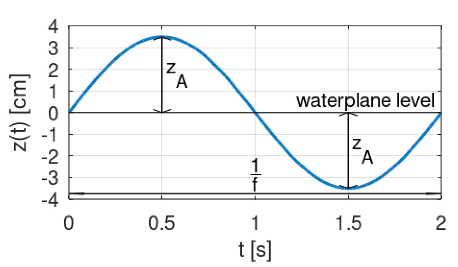
Figure 4.
The water wave (f) is considered a summation of two-dimensional progressive sinusoidal waves harmonics with amplitudes of 3.5 cm and frequencies of: (a) 0.4 Hz, (b) 0.5 Hz, (c) 0.6 Hz, (d) 0.7 Hz, (e) 0.8 Hz.
Figure 4.
The water wave (f) is considered a summation of two-dimensional progressive sinusoidal waves harmonics with amplitudes of 3.5 cm and frequencies of: (a) 0.4 Hz, (b) 0.5 Hz, (c) 0.6 Hz, (d) 0.7 Hz, (e) 0.8 Hz.

Figure 5.
Structural diagram of the developed fuzzy-control system.
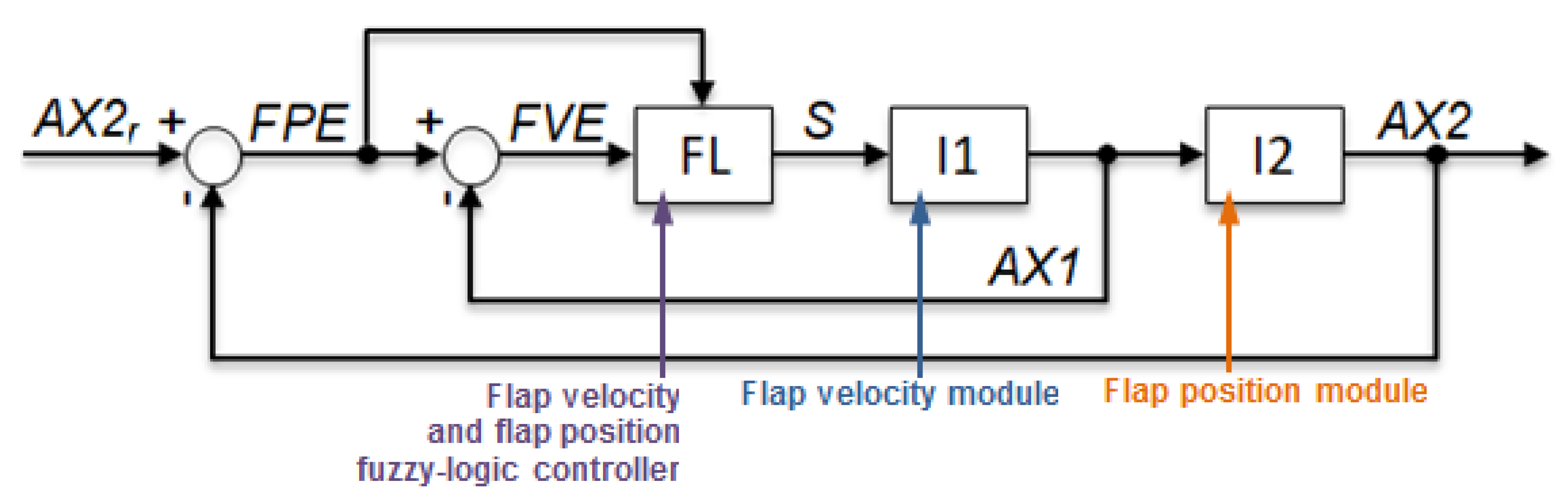
Figure 6.
The fuzzy sets defined as: NF, NM, ZO, PM, PF, with specified membership functions of the L-, - or -type.
Figure 6.
The fuzzy sets defined as: NF, NM, ZO, PM, PF, with specified membership functions of the L-, - or -type.

Figure 7.
The fuzzy sets defined as: NL, NM, ZO, PM, PL, with specified membership functions of the L-, - or -type.
Figure 7.
The fuzzy sets defined as: NL, NM, ZO, PM, PL, with specified membership functions of the L-, - or -type.

Figure 8.
The fuzzy sets defined as: PL, PM, ZO, NM, NL, with membership functions of the -type.

Figure 9.
Output control surface of the fuzzy-logic (FL) controller developed.
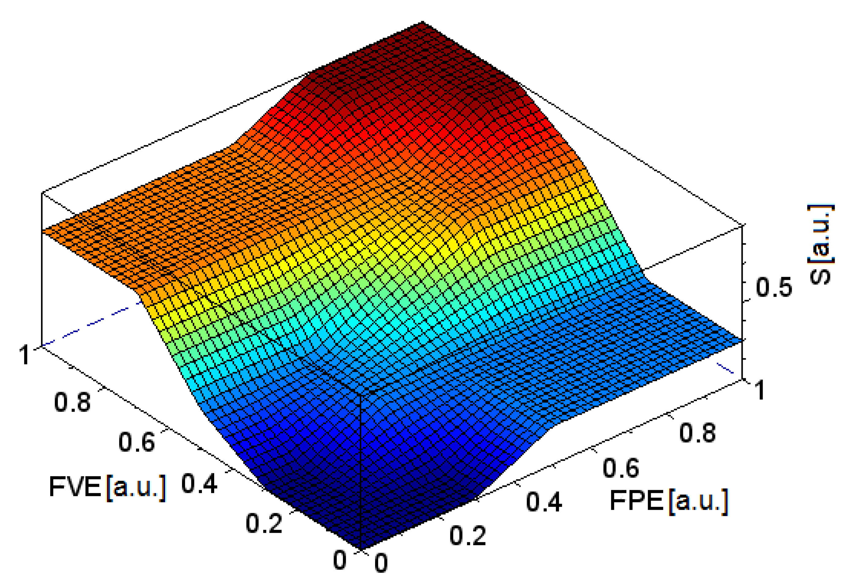
Figure 10.
Trajectories for the initial states of state variables for the model with the fuzzy-logic controller.
Figure 10.
Trajectories for the initial states of state variables for the model with the fuzzy-logic controller.
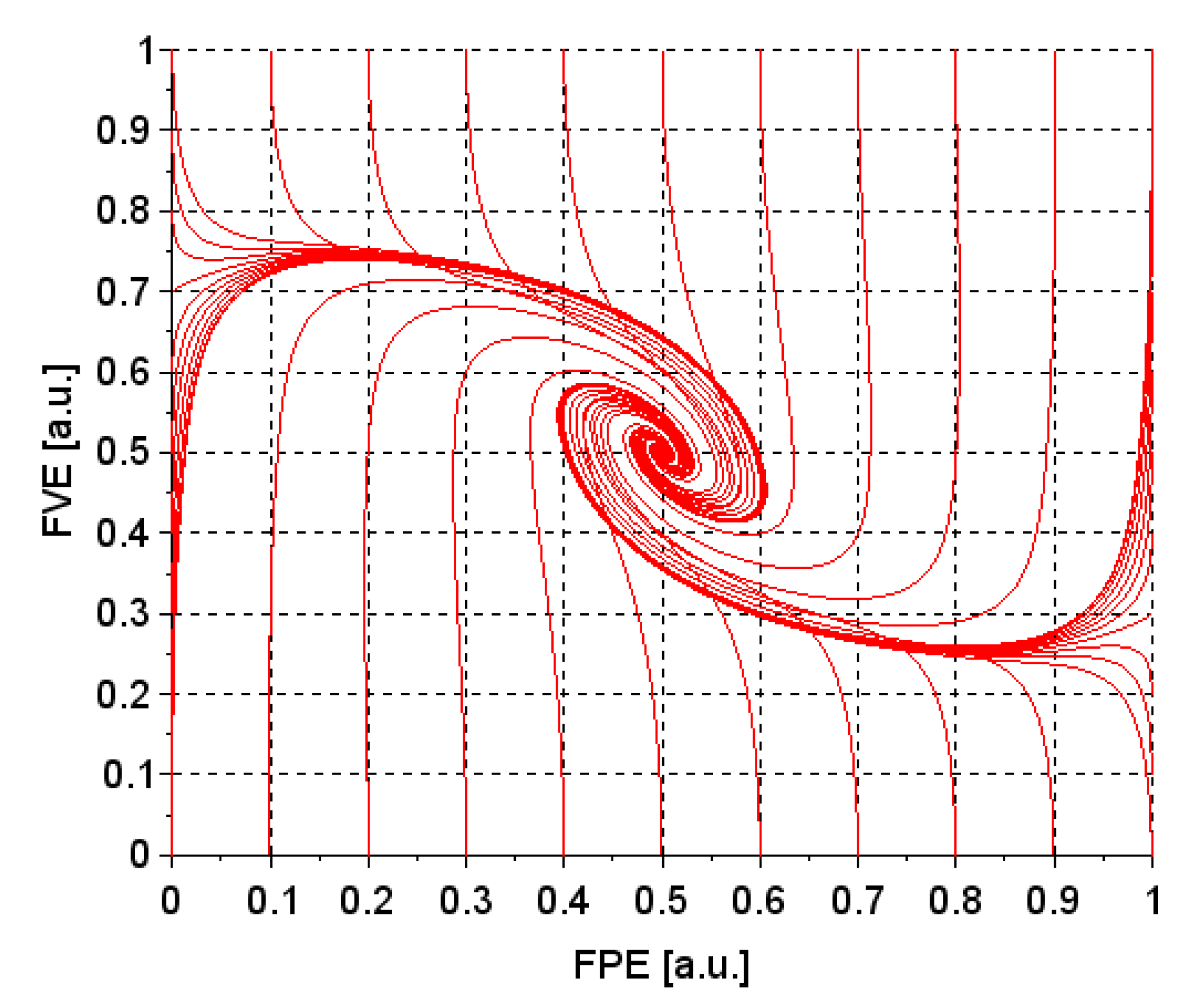
Figure 11.
The wave maker embedded system, equipped with a Graphical User Interface [7].
Figure 11.
The wave maker embedded system, equipped with a Graphical User Interface [7].

Figure 12.
The structural diagram of the measurement system used for the measurement of waves: the measurement ultra-sound device USP50, installed to a towing carriage TB, wireless Bluetooth modules BT for transmission of the measured signal HW and the data acquisition module S8 with a personal computer PC.

Figure 13.
The profiles of the waves generated under the PI controllers and FL controller with desired wave amplitude of 3.5 cm and frequencies of: (a) 0.4 Hz, (b) 0.5 Hz, (c) 0.6 Hz, (d) 0.7 Hz, (e) 0.8 Hz.
Figure 13.
The profiles of the waves generated under the PI controllers and FL controller with desired wave amplitude of 3.5 cm and frequencies of: (a) 0.4 Hz, (b) 0.5 Hz, (c) 0.6 Hz, (d) 0.7 Hz, (e) 0.8 Hz.

Figure 14.
The amplitude spectra of the waves generated under the PI controllers and FL controller with desired wave amplitude of 3.5 cm and frequencies of: (a) 0.4 Hz, (b) 0.5 Hz, (c) 0.6 Hz, (d) 0.7 Hz, (e) 0.8 Hz.
Figure 14.
The amplitude spectra of the waves generated under the PI controllers and FL controller with desired wave amplitude of 3.5 cm and frequencies of: (a) 0.4 Hz, (b) 0.5 Hz, (c) 0.6 Hz, (d) 0.7 Hz, (e) 0.8 Hz.

Figure 15.
The Pierson-Moskowitz spectra for 5th state of sea in North Atlantic for model scale equal to 1:20—the reference (black lines) and generated under the PI controllers and FL controller (blue bars).
Figure 15.
The Pierson-Moskowitz spectra for 5th state of sea in North Atlantic for model scale equal to 1:20—the reference (black lines) and generated under the PI controllers and FL controller (blue bars).

Figure 16.
The amplitude-frequency characteristics of the energy transformation process carried out with the FL controller versus the PI controllers for the desired reference RF—the progressive sinusoidal waves.
Figure 16.
The amplitude-frequency characteristics of the energy transformation process carried out with the FL controller versus the PI controllers for the desired reference RF—the progressive sinusoidal waves.
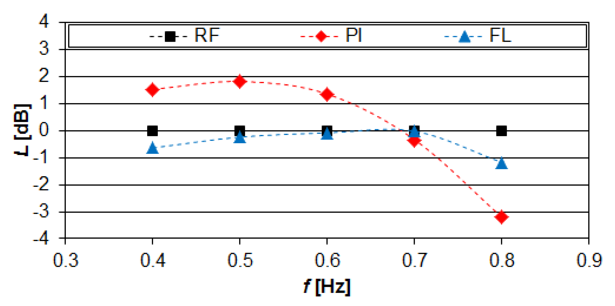
Figure 17.
The amplitude-frequency characteristics of the energy transformation process carried out with the FL controller versus the PI controllers for the desired reference RF—the Pierson-Moskowitz spectra for 5th state of sea in North Atlantic for model scale equal to 1:20.
Figure 17.
The amplitude-frequency characteristics of the energy transformation process carried out with the FL controller versus the PI controllers for the desired reference RF—the Pierson-Moskowitz spectra for 5th state of sea in North Atlantic for model scale equal to 1:20.


Table 1.
Table of the fuzzy rules of the fuzzy inference system developed.
| NL(FPE) | NM(FPE) | ZO(FPE) | PM(FPE) | PL(FPE) | |
|---|---|---|---|---|---|
| PF(FVE) | PM(S) | PM(S) | PM(S) | PL(S) | PL(S) |
| PM(FVE) | PM(S) | PM(S) | PM(S) | PM(S) | PL(S) |
| ZO(FVE) | NM(S) | NM(S) | ZO(S) | PM(S) | PM(S) |
| NM(FVE) | NL(S) | NM(S) | NM(S) | NM(S) | NM(S) |
| NF(FVE) | NL(S) | NL(S) | NM(S) | NM(S) | NM(S) |
Table 2.
The harmonic amplitudes of the progressive sinusoidal waves generated with the fuzzy-logic FL versus proportional-integral PI control algorithms.
Table 2.
The harmonic amplitudes of the progressive sinusoidal waves generated with the fuzzy-logic FL versus proportional-integral PI control algorithms.
| No. | f | (PI) | (FL) | |
|---|---|---|---|---|
| - | Hz | cm | cm | cm |
| 1 | 0.4 | 4.18 | 3.25 | 3.5 |
| 2 | 0.5 | 4.32 | 3.41 | 3.5 |
| 3 | 0.6 | 4.09 | 3.47 | 3.5 |
| 4 | 0.7 | 3.37 | 3.49 | 3.5 |
| 5 | 0.8 | 2.42 | 3.06 | 3.5 |
Table 3.
Table of the measured parameters of the progressive sinusoidal waves generated with the fuzzy-logic FL versus proportional-integral PI control algorithms.
Table 3.
Table of the measured parameters of the progressive sinusoidal waves generated with the fuzzy-logic FL versus proportional-integral PI control algorithms.
| No. | f | L(PI) | L(FL) |
|---|---|---|---|
| - | Hz | dB | dB |
| 1 | 0.4 | 1.54 | −0.63 |
| 2 | 0.5 | 1.83 | −0.23 |
| 3 | 0.6 | 1.36 | −0.08 |
| 4 | 0.7 | −0.34 | −0.02 |
| 5 | 0.8 | −3.21 | −1.18 |
© 2020 by the authors. Licensee MDPI, Basel, Switzerland. This article is an open access article distributed under the terms and conditions of the Creative Commons Attribution (CC BY) license (http://creativecommons.org/licenses/by/4.0/).
Share and Cite
MDPI and ACS Style
Drzewiecki, M.; Guziński, J. Fuzzy Control of Waves Generation in a Towing Tank. Energies 2020, 13, 2049. https://doi.org/10.3390/en13082049
AMA Style
Drzewiecki M, Guziński J. Fuzzy Control of Waves Generation in a Towing Tank. Energies. 2020; 13(8):2049. https://doi.org/10.3390/en13082049
Chicago/Turabian StyleDrzewiecki, Marcin, and Jarosław Guziński. 2020. "Fuzzy Control of Waves Generation in a Towing Tank" Energies 13, no. 8: 2049. https://doi.org/10.3390/en13082049
Note that from the first issue of 2016, this journal uses article numbers instead of page numbers. See further details here.