Abstract
In recent years, China’s terminal clean power replacement construction has experienced rapid development, and China’s installed photovoltaic and wind energy capacity has soared to become the highest in the world. Precise and effective prediction of the scale of terminal clean power replacement can not only help make reasonable adjustments to the proportion of clean power capacity, but also promote the reduction of carbon emissions and enhance environmental benefits. In order to predict the prospects of China’s terminal clean energy consumption, first of all, the main factors affecting the clean power of the terminal are screened by using the grey revelance theory. Then, an evolutionary game theory (EGT) optimized least squares support vector machine (LSSVM) machine intelligence algorithm and an adaptive differential evolution (ADE) algorithm are applied in the example analysis, and empirical analysis shows that this model has a strong generalization ability, and that the prediction result is better than other models. Finally, we use the EGT–ADE–LSSVM combined model to predict China’s terminal clean energy consumption from 2019 to 2030, which showed that the prospect of China’s terminal clean power consumption is close to forty thousand billion KWh.
1. Introduction
With the comprehensive deepening of China’s power industry, the “Thirteenth Five-Year Plan” outline has addressed the major challenges of industrial transformation and put forward a plan for institutional reforms and upgrades in the next 5 years. The “13th Five-Year Plan” outline clearly proposes to promote revolution in four aspects, including energy consumption, supply, technology, and systems. Meanwhile, by 2020, the proportion of non-fossil energy in primary energy consumption must reach 15% [1]. The world’s largest wind and photovoltaic market is in China and clean energy based on photovoltaic and wind power will continue to develop rapidly [2]. In 2019, the Chinese government actively developed photovoltaic and wind power-related construction without subsidy and parity in on-grid projects, fully implemented the competitive allocation mechanism for wind power and photovoltaic power plant projects, and established a new mechanism for renewable energy power consumption. All related policies promote the high-quality development of renewable energy sources. The clean energy power generation installations currently used in China mainly include wind energy, photovoltaic and biomass energy. According to “China Energy Development Report 2019” [3], from the perspective of power generation, in 2019, China’s installed clean energy capacity reached 728 million kilowatts, with an increase of 12%. Among them, the installed hydropower capacity was 352 million kilowatts, the installed wind power capacity was 184 million kilowatts, the installed capacity of photovoltaic power generation was 174 million kilowatts, and the installed capacity of biomass power generation was 17.81 million kilowatts. These values increased by 2.5%, 12.4%, 34%, and 20.7%, respectively, which can be shown in Figure 1.
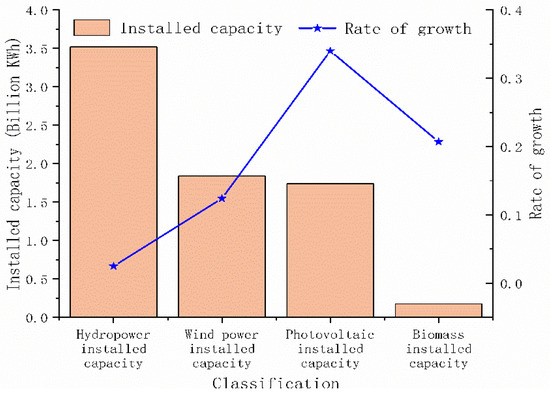
Figure 1.
The installed capacity proportion of clean energy power generation.
From the perspective of terminal consumption, in 2019, China’s total power consumption was 6.8 trillion KWh, of which wind power consumption was 395.7 billion KWh, and wind energy idle generation was 27.7 billion KWh, with a decrease of 14.2 billion KWh. The wind idle rate was 7%, with a decrease of 5%. At the same time, China’s photovoltaic consumption was 183 billion KWh, and the idle amount of photovoltaic power was 5.49 billion KWh, which was 1.8 billion KWh lower than the previous year. China’s hydropower consumption was 138.2 billion KWh, and the idle amount of water power was about 69.1 billion KWh. The national average water idle rate was 5%, with a decrease of 1.8%. China’s biomass power consumption is 283.3 billion KWh. The proportion of terminal clean power consumption is shown in Figure 2.
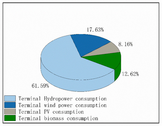
Figure 2.
The proportion of terminal clean power consumption.
In order to accurately predict the scale of future terminal clean electricity consumption in China and provide planning and decision-making assistance for the Chinese government’s energy strategy reform, this paper presents a combined least squares support vector machine (LSSVM) model based on evolutionary game theory and adaptive differential evolution. The algorithm is fully trained and has a good prediction accuracy performance. The rest of the article will be structured as follows: Section 2 reviews the literature from related fields of study in recent years to further clarify the meaning and research method of the paper; Section 3 introduces the mathematical principles of LSSVM, adaptive differential evolution (ADE) and evolutionary game theory (EGT), and the overall algorithm programming process; in Section 4, the proposed EGT–ADE–LSSVM model is fully trained to reach the level of accurate prediction, and applied to China’s terminal clean electricity through a comparison with the prediction results of a traditional backpropagation neural network (BP), LSSVM and ADE–LSSVM algorithms. An empirical analysis is carried out to prove that this paper proposes an intelligent model with a better prediction performance than other models. Finally, the model is used to predict China’s terminal clean electricity consumption prospects for 2019–2030. Section 5 offers a conclusion.
2. Literature Review
Firstly, the prediction of terminal clean power consumption is a multi-dimensional complex system forecasting problem. At present, many scholars have used traditional prediction methods to study energy consumption and other issues, such as grey prediction theory [4,5], multiple regression [6,7,8,9], fuzzy judgment [10,11], etc. However, with the development of machine intelligence algorithms, the prediction accuracy of traditional prediction methods does not meet the needs of development [12]. Compared with traditional prediction methods, intelligent machine algorithms are more and more widely used in the prediction of energy planning. Among them, the LSSVM is the most frequently applied intelligent algorithm [13]. The LSSVM is an improved standard support vector machine (SVM) algorithm based on the least squares function and equality constraints [14]. Compared with standard support vector machines, it has a better prediction performance [15]. Wu et al. [16] used the Cloud-Based Evolutionary Algorithm (CBEA) to optimize LSSVM parameters, including penalty coefficient C and the radial basis kernel function parameter σ, and also verified that the model, after optimizing parameters, is better at predicting the power generation of wind turbines. Because the LSSVM uses equation constraints, Tan et al. [17] minimized the value. The multiplication system is defined as the objective function, thereby simplifying the prediction algorithm process and accelerating the prediction speed of wind turbines. De et al. [18] used the gray system (GM) model and SVM to realize the future of China’s carbon emissions. It was found that the combined model works better. Ahmad et al. [19] analyzed in detail the application of the LSSVM and the packet data processing method in different prediction scenarios. Moreover, they proposed a combined model to predict the energy consumption of buildings with convincing results. De Giorgi et al. [20] used the LSSVM model to predict the photovoltaic power generation situation, and found that the combined prediction model has an optimized performance and successfully predicted 24h photovoltaic power generation.
Through our literature review, we found that, with different combinations of algorithms, a large improvement in the prediction effect of a single machine can be achieved. Liu et al. [21] combined the other algorithms to optimize the LSSVM algorithm. The prognostics health management (PHM) algorithm was used to predict the seasonal factor. Then, the combined PHM–LSSVM algorithm was used to model the equipment failure rate and good experimental results were obtained. Ying [22], in order to optimize the LSSVM, used the ant colony algorithm to realize the assessment of a college cyber security field. Karaboga et al. [23] studied the ant colony, bird swarm and other biological behavior mechanisms, and found that the artificial bee colony was surrounded by bee colony intelligence. They used the artificial bees group (ABG) algorithm to optimize multivariate functions. After comparison, it was found that the ABG algorithm has better results than traditional algorithms, such as the particle swarm optimization (PSO) algorithm. Zhao et al. [24] adopted the latest natural heuristic optimization method, namely the whale optimization algorithm (WOA) to search for the optimal values of two parameters of LSSVM; the algorithm can accurately predict future carbon emission trends, reflecting the applicational value of the combined algorithm. Yang et al. [25] described the basic principles of the PSO in detail, and various improvements to and applications of the PSO were introduced. A process for obtaining multiple prediction models using the PSO algorithm was proposed. Trelea et al. [26] analyzed the performance of the PSO algorithm. The application of the PSO algorithm to the optimization of LSSVM parameters laid an important foundation. Liu et al. [27] proposed an improved gravity search algorithm (AC–GSA) to optimize LSSVM parameters in order to artificially improve the GSA’s performance. They used a new model to predict the thermal efficiency of a 600mw supercritical unit. The results show that the AC–GSA–LSSVM model is very effective for load forecasting. Gorjaei et al. [28] applied the LSSVM model to the prediction of two-phase flow in a wellhead packer and optimized two parameters of the LSSVM algorithm by using particle swarm optimization (PSO). The PSO–LSSVM model is very consistent with the actual measurement rate. The results show that the PSO–LSSVM model has good regression accuracy and generalization ability. Zhang [29] proposed a hybrid model that combines fuzzy clustering (FC), LSSVM, and the wolf pack algorithm (WPA), and tested the data on two cases. Test results show that the model has a high prediction accuracy and stability. Huan et al. [30] proposed a prediction model based on integrated empirical mode decomposition (EEMD) and LSSVM. The results show that the EEMD–LSSVM model is better than the wavelet denoising least squares support vector machine (WD–LSSVM) and the traditional LSSVM. Xue [31] optimized the LSSVM with an improved particle swarm optimization algorithm (IMPSO–LSSVM) and proposed a prediction model for the combined concrete compressive strength.
In recent years, evolutionary game theory (EGT) has been extensively applied in parameter optimization algorithms. In EGT, each participant is an anonymous and random game. Gintis [32] proposed EGT, which utilized the strategic behavior of game theory modeling based on a problem, and described the modeling process of evolutionary game theory in detail. Myerson [33] explained the core points of EGT, and put forward concerns about the process of building the model, laying the foundation for the application of later EGT models. The authors in [33,34] clearly defined the application direction of EGT. Zhang et al. [35] used the EGT model to model the problem of freeway accidents, and the number of accidental escapes was obtained. Therefore, EGT has been widely used in combination parameter selection, and evolutionary game theory is increasingly being introduced into intelligent algorithms [36]. Li et al. [37] used evolutionary stabilization strategies to mathematically coordinate the decision-making between private institutions and humanitarian organizations. The results showed that trust had a significant positive impact on promoting coordination. Selten [38] defined and classified asymmetric animal populations and modeled their evolution using large-scale data analysis. The evolution results of evolutionary games were obtained. Marzband et al. [39] applied evolutionary game theory modeling to integrated energy management systems, and considered a price bidding strategy based on the Nash equilibrium mechanism to clarify the supplier’s response strategy after the game. Similarly, Xiao [40] proposed a new algorithm based on evolutionary game theory to solve the dynamic layout of virtual machines in energy centers and optimize the power consumption of energy centers. This modeling solution can reach theoretical optimality. Cai [41] applied a multi-person asymmetric evolutionary game model optimized by system dynamics to the governance of corporate environmental pollution problems. Simulation results showed that the gold factor is closely related to the limit of fines. Zhu et al. [42] modeled the relationship between Chinese local governments through evolutionary game theory and production enterprises, and analyzed their respective costs and benefits.
3. Mathematical Principle of Forecasting Model
3.1. LSSVM
In order to solve the convex quadratic programming problem in the support vector machine algorithm, the square error term is introduced to transform it into a set of linear equations. This method transforms the inequality constraint problem in the classic support vector machine algorithm into an equality constraint problem, which is helpful in reducing the difficulty of solving [42].
In a set of training samples, , is the input vector of the n-dimensional integral energy of each system, is the output vector of the LSSVM model, is the number of training samples.
The LSSVM model can be expressed in the feature space as follows:
where is a nonlinear mapping function, is a weight vector in a feature space and is the amount of offset.
According to the principle of structural risk minimization, the function estimation of LSSVM can be described as:
where is the punishing parameters for the error, indicates the error variable, .
The constraint can be expressed as follows:
In order to extract the original spatial features of each system, this paper constructs a nonlinear mapping function in the original space to the highly dimensional space. According to (2), a Lagrangian equation can be defined as follows.
where is the Lagrange multiplier, .
According to KarushKuhnTucker (KKT) conditions, (4) makes the following optimizations:
It can be known from Equation (5) that the value of each component is non-zero and is proportional to the error of the data sampling point. Therefore, the above problem can be transformed into a (n + 1) dimensional linear equation problem. By using the method of eliminating the weight vector of the feature space and error variables , we get the matrix equation:
where ,, is a unit matrix and is a kernel function.
According to the Mercer condition, there are mapping and kernel functions .
We get after calculating the combination of (6) and (7), and the regression function of the comprehensive prediction data of energy system is:
Therefore, we get the output function of the LSSVM model:
3.2. Adaptive Differential Evolution Algorithm
Adaptive differential evolution (ADE) is a heuristic random search algorithm that simulates the evolutionary differences of populations. The performance of the ADE algorithm is highly dependent on mutation strategies and controlling parameters, including population size , scaling factor and cross constants . The ADE algorithm has four steps, including initialization, mutation operation, cross operation and selection operation.
3.2.1. Initialization
Let the population size be ; if the dimension of the feasible solution space is , then use to indicate , the generation population.
Each individual is made up of dimensional parameters, which can be expressed as:
3.2.2. Mutation Operation
Individuals in the parent population can mutate to individuals through mutation operations. Two different groups were randomly selected in the population and their vectors were scaled to perform vector synthesis with the individual to be mutated:
where is the scaling factor, whose value range is from 0 to 1 [0,1]. is the randomly selected basis vector to be perturbed. is the difference vector.
3.2.3. Cross Operation
The generated mutant individuals are crossed with the individuals of the original population to form new crossed individuals. The binomial crossed operation is:
where . is a random number from 0 to 1 in [0,1]. is the cross constant from 0 to 1 of [0,1].
3.2.4. Selection Operation
The selection operation follows the greedy genetic model of survival of the fittest, so individual offspring are always better than their parents or at least equal to their parents—that is, only when the fitness value of the individual of the new vector is greater than the fitness value of the target vector individual will the new vector individuall be accepted; otherwise, still remains in the next generation population, and continues to perform mutation and crossover operations as target vectors in the next iteration. The selection operation is as follows:
where is the optimized objective function.
Due to the fact that the population size range is fixed, the mutation factor and cross-factor are automatically adapted according to Equation (15) during the iterative process of evolution, and the optimal results are finally generated, as shown in Equations (16) and (17). During the continuous iteration of the program, the population tends to the optimal solution during evolution, the population favors the optimal solution during evolution, and the best mutation factors and cross-factors are allocated:
where and are the probability of regulating and , respectively.
Because and affect each other, the optimal values of these two parameters can be obtained after multiple simulation experiments. This article sets these two parameters as follows:
where is a normal random distribution datum with a mean of 0.5 and a deviation of 0.3.
3.3. Evolutionary Game Theory
The core idea of evolutionary game theory is that people are not completely rational, but rather that they establish a corresponding decision set through a trial and error mechanism. Therefore, the idea of evolutionary game theory is introduced in the adaptive differential evolution algorithm in this paper. The steps of evolutionary game theory are as follows.
Step 1: Set as the utility function when the opponent uses strategy , taking as the strategy. Then, the stable conditions of evolution are as follows [41]:
There are two populations, and , and their respective utility functions are:
By playing against its own parent generation individuals, each population calculates its own average individual utility to determine its own fitness. The average fitness after the second game is calculated as follows:
Then, the corresponding fitness of the individual can be calculated:
where is the probability that the fitness value of an individual is occupied in the population.
Assume that half of the information comes from a population and the other half comes from the elite solution set. The probability of each individual is , so the probability that the generated children belong to the first population is as follows.
The flow of the EGT algorithm proposed in this paper is shown in Figure 3:
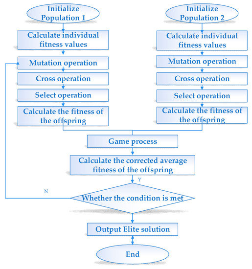
Figure 3.
The flow of evolutionary game theory (EGT) algorithm.
3.4. Combined EGT–ADE–LSSVM Model
In Section 3.3, it is clear that EGT can solve the shortcomings of the ADE algorithm well. In the ADE algorithm, disadvantaged individuals will be avoided after evolution, but these disadvantaged individuals will pass through . After the second evolution, it is also possible to develop in the direction of the optimal solution. Meanwhile, the original superior individual may also proceed in the direction of the inferior solution, which is more in line with evolution in reality. Therefore, EGT can control the ADE algorithm to avoid developing in the direction of a local optimal solution. Therefore, the EGT–ADE algorithm can search for the penalty coefficient c and the radial basis kernel function global value . Due to the fact that the initial parameter penalty coefficient c and the radial basis kernel function of the traditional LSSVM model greatly affect the performance of the prediction model, this article uses the ADE algorithm improved by EGT to perform global search optimization on the parameters in order to increase the accuracy of the LSSVM algorithm.
During the operation of the combined EGT–ADE–LSSVM model, the optimal solution of parameters is always maintained to achieve accurate prediction of terminal clean power consumption in China. The algorithm principle of the clean power consumption prediction model in China based on EGT–ADE–LSSVM is divided into the following steps:
- (1)
- Collect experimental data and initialize all relevant parameters of the EGT–ADE–LSSVM model;
- (2)
- Operate the EGT–ADE algorithm to search for the penalty coefficient c and global value of radial basis kernel function ;
- (3)
- Output the penalty coefficient c and the radial basis kernel function corresponding to the global optimal fitness value into the LSSVM model;
- (4)
- Build training and testing sample sets of the LSSVM model and train multiple training sets;
- (5)
- Output the results of the testing sample sets.
The flow of the EGT–ADE–LSSVM algorithm is shown in Figure 4:
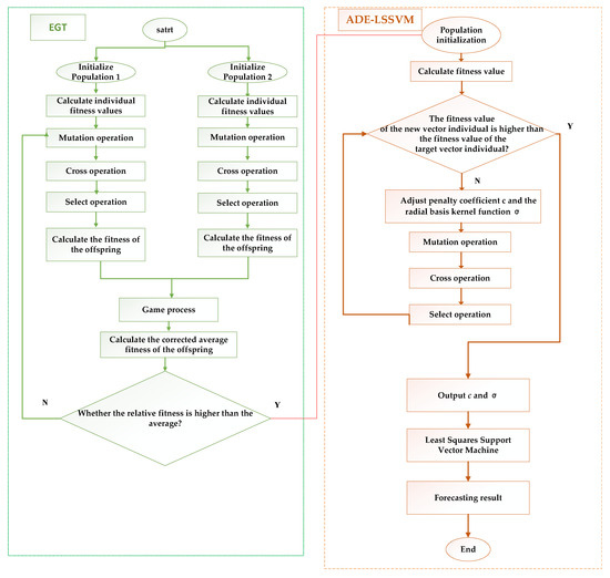
Figure 4.
The EGT–adaptive differential evolution (ADE)–least squares support vector machine (LSSVM) algorithm flow chart.
4. Empirical Analysis
4.1. Influencing Factors Filter Model Input
Using data from the “Energy Consumption” section of the China Statistical Yearbook and the statistical data published on the website of the China Energy Administration, this article selects gross domestic product(GDP), total population, urban population, coal price, GDP of primary industry, GDP of secondary industry, GDP of tertiary industry, net investment in energy industry, net investment in photovoltaic industry, net investment in wind energy industry, net investment in biomass energy industry, net installed wind power capacity, net installed photovoltaic capacity, fixed assets for biomass power generation, net installed capacity and net transmission and transformation investment and distribution network as the influencing factors for China’s terminal clean energy consumption. Grey relevance theory is applied to eliminate some factors with a degree less than 0.4.
4.2. Grey Relevance Theory
The following are the relevant calculation steps for gray correlation theory:
Step 1: Determine the relevant analysis series
Determine the reference and the comparison series that reflect the behavior of the system series. The reference sequence refers to a data sequence that reflects the behavioral characteristics of the system. A series of data, as part of the factors that affect the behavior of the system, is called a comparison series. Assume that the reference number is , and compare the series as follows:
Step 2: Dimensionless variables
Because the data of each factor column in the system may have different dimensions, it is inconvenient to compare these data, and it is difficult to draw the correct conclusion from this comparison. Therefore, in gray correlation theory, the data are usually dimensionless:
Step 3: Calculate the correlation coefficient
Calculate the correlation coefficient of and :
Let , then:
is the resolution coefficient. The smaller , the greater the resolution. Under normal circumstances, the value range of is (0, 1), the specific value depends on the situation. When , the resolution is the best, so we take = 0.4.
Step 4: Calculate the correlation
Because the concept of the correlation coefficient refers to the degree of correlation between the comparison sequence and the reference sequence at each moment (i.e., each point on the curve), the correlation coefficient has a lot of numbers, and too much information is not conducive to the overall comparison, so the correlation coefficient at each time (that is, each point on the curve) needs to be changed into a value, this value is then the average of the numbers, and is expressed as the number of correlations between the comparison sequence and the reference sequence. The correlation Equation is as follows:
Step 5: Relevance ranking
Sort the relevance based on size: if , the reference sequence y is similar to the comparison sequence . The correlation coefficient between the sequence and the sequence are first calculated, and then the average of the correlation coefficients for each type is calculated, which is called the correlation degree between and .
In this paper, grey relevance theory is used to select the main influencing factors that have a large correlation with the clean power consumption of the terminal. The set of influencing factors of terminal clean power consumption is shown in Table 1:

Table 1.
Influencing factors of terminal clean power consumption.
4.3. Data Normalization
In order to eliminate dimensional differences between data of different measures, all the corrected data are normalized. In the data set of M indicators, the Z-score data normalization method is used to correspondingly normalize the N groups of data.
is the normalized data, is the correction data, is the mean of and is the standard deviation of .
For negative indices, this paper uses the inverse exponential positive processing method to obtain positive data:
where is the normalized data, is the maximum value of the normalized data and is the minimum value of the normalized data. Some details of the processed data are shown in Table 2.
Table 2.
Partial normalized data.
4.4. Prediction Result Test of EGT–ADE–LSSVM Model
The data from 1990–2010 were input into the training set of the EGT–ADE–LSSVM model, and the data from 2011 to 2018 were used as the test set. The main parameters of the EGT–ADE–LSSVM model are shown in Table 3.
Table 3.
Key parameters of the EGT–ADE–LSSVM model.
In order to predict the accuracy of the model proposed in this paper, we simultaneously inputted sample data into three prediction models: a backpropagation (BP) neural network, LSSVM, and ADE–LSSVM, and used relative error (ER) to calculate the degree of prediction accuracy. The prediction results obtained by each prediction model are shown in Figure 5:
where is the predicted value and is the actual value.
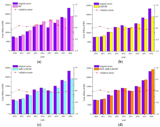
Figure 5.
The predicted results of the test sets: (a) backpropagation (BP) predicted results; (b) the predicted results of LSSVM; (c) the predicted results of ADE–LSSVM; (d) the predicted results of EGT–ADE–LSSVM.
The prediction results of different prediction models are compared as shown in Figure 6.
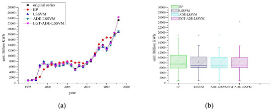
Figure 6.
Forecast comparison of forecast results: (a) the line chart; (b) the box plot.
As can be seen from Figure 5 and Figure 6, this paper proposes a reliable EGT–ADE–LSSVM model that has a good prediction effect.
Through comparative analysis, we found that:
- (1)
- Parameter optimization is of great significance to machine intelligence algorithms, and prediction algorithms without parameter optimization have almost no effect on accurate predictions. Compared with the single model prediction, the fitting effect of the joint prediction model is obviously better. The parameter-optimized model has better prediction capabilities;
- (2)
- Different parameter optimization methods have different effects. The EGT–ADE–LSSVM model is a complex multi-combination prediction model that can achieve the complementary advantages of different algorithms;
- (3)
- Through the EGT–ADE algorithm continuously optimizing the parameters of the LSSVM algorithm, the model proposed in this article has more reasonable parameters than the ADE–LSSVM prediction algorithm.
Through the above analysis, the empirical analysis proves that the intelligent prediction model of the EGT–ADE–LSSVM method proposed in this paper is practical and effective in predicting the total consumption of China’s terminal clean energy.
4.5. Model Output
We applied grey relevance theory to predict the main influencing factors from 2019 to 2030, which were applied as the input data for the EGT–ADE–LSSVM prediction model. Finally, we calculated China’s total terminal clean energy consumption from 2019 to 2030, as shown in Figure 7:
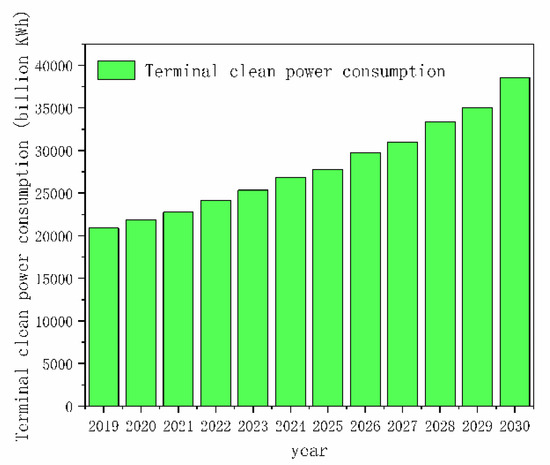
Figure 7.
Output result of EGT–ADE–LSSVM forecasting model.
According to the planned value of the entire power consumption of Chinese society proposed in the 13th Five-Year Plan of China, which is shown in Table A2 in Appendix A section, combined with the terminal clean power consumption forecasted in this paper, which is shown in Table A1 in Appendix A section, the terminal clean power consumption trend of China in the next 10 years is finally obtained, as shown in Figure 8.
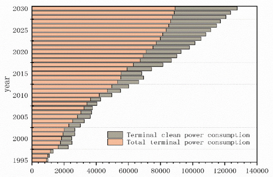
Figure 8.
China’s terminal clean power consumption trend.
It can be seen from the trend in Figure 8 that the proportion of China’s terminal clean power consumption has gradually increased, and it is estimated that, by 2030, this proportion will exceed 38%.
5. Conclusions
This paper first defines terminal clean power consumption, and then proposes an innovative model to realize the extraction of influencing factors and forecast the prospect of China’s terminal clean power consumption. The idea of evolutionary game theory (EGT) is applied to the differential evolution algorithm (ADE) to achieve the two parameters of LSSVM. We used the grey relevance theory to screen and obtain the set of main influencing factors that affect the terminal clean power consumption, and then normalized the original set. Then, we used the EGT theory to improve traditional ADE to form a new differential evolution algorithm and optimize the two parameters of the LSSVM. Using the data from 1995–2009 as the training set and the data from 2010–2018 as the test set, an innovative EGT–ADE–LSSVM forecasting model is used to predict China’s terminal clean power consumption in 2010–2018. In order to verify the validity of this model, the same samples are inputted in the BP, LSSVM and ADE–LSSVM algorithms, etc. The prediction results are considerable, and verify that the EGT–ADE–LSSVM model has a high prediction accuracy and practicality. Finally, China’s terminal clean power consumption and consumption proportion trend is predicted from 2019 to 2030 by using the prediction model and results proposed in this paper indicate that China’s terminal clean energy consumption will reach 38.575 billion kWh in 2030 and the consumption proportion will reach 48.77%, indicating that China has great potential in the consumption of terminal clean power, and can implement the development goals of non-fossil energy production and consumption revolution.
Author Contributions
In this paper, S.Y. collected the relevant data and carried out the empirical analysis, results comparison and wrote the first manuscript. X.Z. and S.P. made improvements to the English and adjusted the article’s structure. All authors have read and agreed to the published version of the manuscript.
Funding
The research was funded by the National Social Science Foundation of China (NO.16BJY055).
Conflicts of Interest
The authors declare no conflict of interest.
Appendix A
Table A1.
The amount of terminal clean power consumption.
Table A1.
The amount of terminal clean power consumption.
| Year | Terminal Clean Power Consumption | Year | Terminal Clean Power Consumption | Year | Terminal Clean Power Consumption |
|---|---|---|---|---|---|
| 1995 | 984.342 | 2007 | 5251.946 | 2019 | 20,893.24 |
| 1996 | 1037.455 | 2008 | 6238.959 | 2020 | 21,845.56 |
| 1997 | 1781.532 | 2009 | 6313.943 | 2021 | 22,756.63 |
| 1998 | 6311.942 | 2010 | 7757.743 | 2022 | 24,093.99 |
| 1999 | 7191.492 | 2011 | 8019.884 | 2023 | 25,338.03 |
| 2000 | 6400.462 | 2012 | 10,549.54 | 2024 | 26,876.35 |
| 2001 | 7299.04 | 2013 | 13,210.97 | 2025 | 27,753.36 |
| 2002 | 6571.945 | 2014 | 14,179.75 | 2026 | 29,765.46 |
| 2003 | 7155.944 | 2015 | 12,757.53 | 2027 | 30,967.56 |
| 2004 | 7245.492 | 2016 | 15,240.43 | 2028 | 33,379.04 |
| 2005 | 7916.042 | 2017 | 18,404.24 | 2029 | 35,045 |
| 2006 | 6693.04 | 2018 | 19,435.61 | 2030 | 38,575.03 |
Table A2.
The amount of total terminal power consumption.
Table A2.
The amount of total terminal power consumption.
| Year | Total Terminal Power Consumption | Year | Total Terminal Power Consumption | Year | Total Terminal Power Consumption |
|---|---|---|---|---|---|
| 1995 | 9002 | 2007 | 32,458 | 2019 | 69,230 |
| 1996 | 9864 | 2008 | 34,268 | 2020 | 71,000 |
| 1997 | 11,454 | 2009 | 36,430 | 2021 | 75,320 |
| 1998 | 16,345 | 2010 | 41,923 | 2022 | 77,342 |
| 1999 | 17,734 | 2011 | 47,022 | 2023 | 79,932 |
| 2000 | 18,334 | 2012 | 49,657 | 2024 | 81,342 |
| 2001 | 19,344 | 2013 | 53,233 | 2025 | 83,544 |
| 2002 | 20,093 | 2014 | 55,233 | 2026 | 85,134 |
| 2003 | 22,945 | 2015 | 55,500 | 2027 | 86,332 |
| 2004 | 25,349 | 2016 | 59,198 | 2028 | 87,324 |
| 2005 | 28,353 | 2017 | 63,077 | 2029 | 88,543 |
| 2006 | 30,435 | 2018 | 67,403 | 2030 | 89,110 |
References
- Promoting the Development of High Proportion of Renewable Energy. Available online: http://www.creei.cn/portal/article/index/id/23793/cid/6.html (accessed on 8 October 2019).
- BP Statistical Review of World Energy. Available online: https://www.bp.com/content/dam/bp/en/corporate/pdf/energy-economics/statistical-review/bp-stats-review-2018-full-report.pdf (accessed on 4 June 2019).
- China-2050-High-Renewable-Energy-Penetration-Scenario-and-Roadmap-Study-Executive-Summary. Available online: http://www.cnrec.org.cn/go/AttachmentDownload.aspx?id={314648b5-6dcd-43f8-9903-db1ac953cc55} (accessed on 7 October 2019).
- Alessandrini, S.; Monache, L.D.; Sperati, S.; Nissen, J.N. A novel application of an analog ensemble for short-term wind power forecasting. Renew. Energy 2015, 76, 768–781. [Google Scholar] [CrossRef]
- Zhang, Y.G.; Wang, S.; Gao, Y.L. A Novel Wind Power Generation Capacity Prediction Technique Based on Optimal Combination Forecasting Method. Control Eng. China 2016, 23, 992–996. [Google Scholar]
- Treiber, N.A.; Kramer, O. Evolutionary feature weighting for wind power prediction with nearest neighbor regression. In Proceedings of the Evolutionary Computation, Sendai, Japan, 25–28 May 2015. [Google Scholar]
- Zhao, Y.; Ye, L.; Li, Z.; Song, X.; Lang, Y.; Su, J. A novel bidirectional mechanism based on time series model for wind power forecasting. Appl. Energy 2016, 177, 793–803. [Google Scholar] [CrossRef]
- Eldali, F.A.; Hansen, T.M.; Suryanarayanan, S.; Chong, E.K.P. Employing ARIMA models to improve wind power forecasts: A case study in ERCOT. In Proceedings of the 9th American Power Symposium, Denver, CO, USA, 18–20 September 2016. [Google Scholar]
- Li, W.; Zhang, H.T.; An, T.T. Study on Short-Term Wind Power Prediction Model Based on ARMA Theory. Appl. Mech. Mater. 2013, 448–453, 1875–1878. [Google Scholar] [CrossRef]
- YiShian, L.; Leelng, T. Forecasting energy consumption using a grey model improved by incorporating genetic programming. Energ. Convers. Manag. 2011, 52, 147–1152. [Google Scholar]
- Li, M.; Wang, W.; De, G.; Ji, X.; Tan, Z. Forecasting Carbon Emissions Related to Energy Consumption in Beijing-Tianjin-Hebei Region Based on Grey Prediction Theory and Extreme Learning Machine Optimized by Support Vector Machine Algorithm. Energies 2018, 11, 2475. [Google Scholar] [CrossRef]
- Liu, Y.; Sun, Y.; Infield, D.; Zhao, Y.; Han, S.; Yan, J. A hybrid forecasting method for wind power ramp based on orthogonal test and support vector machine (OT-SVM). IEEE Trans. Sustain. Energy 2017, 8, 451–457. [Google Scholar] [CrossRef]
- Tian, Z.; Li, S.; Wang, Y.; Wang, X. Wind power prediction method based on hybrid kernel function support vector machine. Wind Eng. 2017, 42, 252–264. [Google Scholar] [CrossRef]
- Li, X.; Wang, X.; Zheng, Y.H.; Li, L.X.; Zhou, L.D.; Sheng, X.K. Short-Term Wind Power Forecasting Based on Least-Square Support Vector Machine (LSSVM). Appl. Mech. Mater. 2013, 448, 1825–1828. [Google Scholar] [CrossRef]
- Zhao, H.; Guo, S.; Zhao, H. Energy-Related CO2 Emissions Forecasting Using an Improved LSSVM Model Optimized by Whale Optimization Algorithm. Energies 2017, 10, 874. [Google Scholar] [CrossRef]
- Wu, Q.; Peng, C. A Least Squares Support Vector Machine Optimized by Cloud-Based Evolutionary Algorithm for Wind Power Generation Prediction. Energies 2016, 9, 585. [Google Scholar] [CrossRef]
- Tan, Z.; De, G.; Li, M.; Lin, H.; Yang, S.; Huang, L.; Tan, Q. Combined electricity-heat-cooling-gas load forecasting model for integrated energy system based on multi-task learning and least square support vector machine. J. Clean. Prod. 2019, 248, 119252. [Google Scholar] [CrossRef]
- De, G.; Tan, Z.; Li, M.; Huang, L.; Wang, Q.; Li, H. A credit risk evaluation based on intuitionistic fuzzy set theory for the sustainable development of electricity retailing companies in China. Energy Sci. Eng. 2019, 7, 2825–2841. [Google Scholar] [CrossRef]
- Ahmad, A.S.B.; Hassan, M.Y.B.; Majid, M.S.B. Application of hybrid GMDH and Least Square Support Vector Machine in energy consumption forecasting. In Proceedings of the IEEE International Conference on Power and Energy, Kota Kinabalu, Malaysia, 2–5 December 2012. [Google Scholar]
- De Giorgi, M.G.; Malvoni, M.; Congedo, P.M. Comparison of strategies for multi-step ahead photovoltaic power forecasting models based on hybrid group method of data handling networks and least square support vector machine. Energy 2016, 107, 360–373. [Google Scholar] [CrossRef]
- Liu, H.Y.; Jiang, Z.J. Research on Failure Prediction Technology Based on Time Series Analysis and ACO-LSSVM. Comput. Mod. 2013, 1, 219–222. [Google Scholar] [CrossRef]
- Ying, E. Network Safety Evaluation of Universities Based on Ant Colony Optimization Algorithm and Least Squares Support Vector Machine. J. Converg. Inf. Technol. 2012, 7, 419–427. [Google Scholar]
- Karaboga, D.; Basturk, B. A powerful and efficient algorithm for numerical function optimization: Artificial bee colony (ABC) algorithm. J. Glob. Optim. 2007, 39, 459–471. [Google Scholar] [CrossRef]
- Cheng, R.H.; Chen, D.W.; Gai, W.L.; Zheng, S. Intelligent driving methods based on sparse LSSVM and ensemble CART algorithms for high-speed trains. Comput. Ind. Eng. 2019, 1, 1203–1213. [Google Scholar] [CrossRef]
- Yang, W.; Li, Q. Survey on Particle Swarm Optimization Algorithm. Eng. Sci. 2004, 6, 87–94. [Google Scholar]
- Trelea, I.C. The particle swarm optimization algorithm: Convergence analysis and parameter selection. Inform. Process. Lett. 2016, 85, 317–325. [Google Scholar] [CrossRef]
- Liu, C.; Niu, P.; Li, G.; You, X.; Ma, Y.; Zhang, W. A Hybrid Heat Rate Forecasting Model Using Optimized LSSVM Based on Improved GSA. Neural Process. Lett. 2017, 45, 299–318. [Google Scholar] [CrossRef]
- Gorjaei, R.G.; Songolzadeh, R.; Torkaman, M.; Safari, M.; Zargar, G. A novel PSO-LSSVM model for predicting liquid rate of two phase flow through wellhead chokes. J. Nat. Gas Sci. Eng. 2015, 24, 228–237. [Google Scholar] [CrossRef]
- Zhang, X. Short-Term Load Forecasting for Electric Bus Charging Stations Based on Fuzzy Clustering and Least Squares Support Vector Machine Optimized by Wolf Pack Algorithm. Energies 2018, 11, 1449. [Google Scholar] [CrossRef]
- Huan, J.; Cao, W.; Qin, Y. Prediction of dissolved oxygen in aquaculture based on EEMD and LSSVM optimized by the Bayesian evidence framework. Comput. Electron. Agric. 2018, 150, 257–265. [Google Scholar] [CrossRef]
- Xue, X. Evaluation of concrete compressive strength based on an improved PSO-LSSVM model. Comput. Concr. 2018, 21, 501–511. [Google Scholar]
- Gintis, H. Game Theory Evolving: A Problem-Centered Introduction to Modeling Strategic Behavior; Princeton University Press: Princeton, NJ, USA, 2000. [Google Scholar]
- Myerson, R.B. Game Theory; Harvard University Press: Cambridge, MA, USA, 2013. [Google Scholar]
- Weibull, J.W. Evolutionary Game Theory; MIT Press: Cambridge, MA, USA, 1997. [Google Scholar]
- Zhang, G.L. Defraud Behavior of Network Toll Highway Based on Evolutionary Game Model. J. Transp. Syst. Eng. Inf. Technol. 2014, 14, 113–119. [Google Scholar]
- Ji, P. Developing green purchasing relationships for the manufacturing industry—An evolutionary game theory perspective. Int. J. Prod. Econ. 2015, 166, 155–162. [Google Scholar] [CrossRef]
- Li, C.; Zhang, F.; Cao, C.; Liu, Y.; Qu, T. Organizational coordination in sustainable humanitarian supply chain: An evolutionary game approach. J. Clean. Prod. 2019, 219, 291–303. [Google Scholar] [CrossRef]
- Selten, R. A note on evolutionarily stable strategies in asymmetric animal conflicts. J. Theor. Biol. 1980, 84, 93–101. [Google Scholar] [CrossRef]
- Marzband, M. Non–cooperative game theory based energy management systems for energy district in the retail market considering DER uncertainties. IET Gener. Trans. Distrib. 2016, 10, 2999–3009. [Google Scholar] [CrossRef]
- Xiao, Z. A solution of dynamic VMs placement problem for energy consumption optimization based on evolutionary game theory. J. Syst. Softw. 2015, 101, 260–272. [Google Scholar] [CrossRef]
- Cai, L.R. Multi–person evolutionary game of environment pollution based on system dynamics. Appl. Res. Comput. 2011, 28, 2982–2986. [Google Scholar]
- Zhu, Q.H. Analysis of an evolutionary game between local governments and manufacturing enterprises under carbon reduction policies based on system dynamics. Oper. Res. Manag. Sci. 2014, 23, 71–82. [Google Scholar]


© 2020 by the authors. Licensee MDPI, Basel, Switzerland. This article is an open access article distributed under the terms and conditions of the Creative Commons Attribution (CC BY) license (http://creativecommons.org/licenses/by/4.0/).