Article

A Comparative Study of Solar-Driven Trigeneration Systems for the Building Sector

by
Christos Tzivanidis
* and
Evangelos Bellos
Thermal Department, School of Mechanical Engineering, National Technical University of Athens, Zografou, Heroon Polytechniou 9, 15780 Athens, Greece
*
Author to whom correspondence should be addressed.
Energies 2020, 13(8), 2074; https://doi.org/10.3390/en13082074
Submission received: 3 April 2020 / Revised: 12 April 2020 / Accepted: 15 April 2020 / Published: 21 April 2020

Abstract

:
The utilization of solar irradiation in the building sector is vital to create sustainable systems. Trigeneration systems are highly efficient systems that usually produce electricity, heating and cooling which are the main energy needs in the buildings. The objective of this work is the energetic and financial investigation of three different solar-driven trigeneration systems that can be applied in buildings with high energy needs (e.g., hospitals or commercial buildings). The parabolic trough solar collector (PTC) is selected to be used because it is the most mature solar concentrating technology. The examined configurations practically are different combinations of organic Rankine cycle (ORC) with heat pumps. System 1 includes a PTC coupled to an ORC which feeds an absorption heat pump machine. System 2 includes a PTC which simultaneously feeds an ORC and absorption machine. System 3 includes a PTC which feeds an ORC and a heat exchanger for heating, while the ORC is fed with and electricity a vapor compression cycle for cooling production. The simple payback period of System 1 is 5.62 years and it is the lowest, with System 2 to have 7.82 years and System 3 to have 8.49 years. The energy efficiency of the three systems is 78.17%, 43.30% and 37.45%, respectively, while the exergy efficiency 15.94%, 13.08% and 12.25%, respectively. System 1 is the best configuration according to energy, exergy and financial analysis. This study is performed with developed thermodynamic models in Engineering Equation Solver and a dynamic model in FORTRAN.

Graphical Abstract

1. Introduction

Solar energy is a vital energy source in order to face critical energy problems such as fossil fuel depletion, global warming, the increasing energy demand and the increasing electricity price [1,2]. The building sector is one of the most energy-consuming sectors of our society and the exploitation of solar irradiation in the buildings is an interesting idea that can lead to future sustainability [3]. Moreover, trigeneration systems are highly efficient units that can produce numerous useful outputs simultaneously [4,5] and usually they can produce the outputs that the building needs (heating, cooling and electricity). So, the use of solar energy for feeding trigeneration systems seems to be a viable and environmentally friendly idea. Especially in buildings with high energy needs, like hospitals and commercial buildings, trigeneration systems can be installed easily without scale restrictions which can be found in residential buildings.
In this direction, there are many literature studies with solar-driven trigeneration configurations for the building sector. The most usual design includes an organic Rankine cycle (ORC) and heat pumps, while the most usual solar technology is the parabolic trough collector (PTC). The heat pumps can be absorption chillers (ACH) or vapor compression cycles (VCC). Al-Sulaiman et al. [6] examined a trigeneration system with ORC and ACH driven by PTC. The ACH is fed by the waste heat after the ORC turbine. They concluded that the exergy efficiency of the system is about 20% and the maximum turbine production is 115 kW. Bellos and Tzivanidis [7] studied a similar configuration with a 1000 m2 collecting area and they stated the optimized case has 152% energy efficiency, 29.4% exergy efficiency and 177.6 kW electricity production. At this point, it is important to state that in the system with heat pumps, the energy efficiency can be over 100% because the cooling load acts as an energy input in the system but it does not take into account the denominator of the energy efficiency definition. In another work, Eisavi et al. [8] studied a configuration with ORC of around 0.5 MWel nominal power and a double-effect absorption heat pump which presents 96% energy efficiency and 12.8% exergy efficiency. Zhao et al. [9] performed a comparative study in order to determine the optimum technique for combining ACH, ORC and PTC. They concluded that feeding the ACH by the ORC’s waste heat is the optimum way for maximizing the exergy efficiency index which is found to be 41%, while the nominal power production of the system is 200 kW. Moreover, Khalid et al. [10] studied a unit with ACH and ORC coupled to the solar field loop. The waste heat of the ORC assists a VCC for heating production. Geothermal energy and wind energy are also used in this system which presents 76.1% energy efficiency, 7.3% exergy efficiency, while the net present value is close to 350 k$ for a nominal electrical power of 30 kW. Bellos et al. [11] investigated a unit with VCC coupled to an ORC which is fed by 70 m2 PTC and biomass fuel. This polygeneration system produced cooling, electricity and heating at two temperature levels. According to their results, the payback period is close to five years, the exergy efficiency 21.8%, the energy efficiency 51.3% and the electricity production is 8.2 kW. Mathkor et al. [12] studied a system that produces fresh-water, cooling and electricity of around 1.2 MW. They found exergy efficiency close to 42% while the electricity capacity is 1 MW, the cooling capacity around 190 tons and the fresh-water production around 130 tons daily. Zhang et al. [13] examined a simple system with ORC, ACH and PTC. They found that the optimum working fluid in the ORC is the MM, while the overall system efficiency is 40.95%. The heating/power ratio was found 4.2 and the cooling/power ratio 4.95, while the gross power production was 200 MW.
Moreover, there are other solar-driven trigeneration systems in the literature. Dabwan et al. [14] investigated different ways to incorporate PTC in a gas turbine trigeneration system. They found that the use of PTC can reduce the levelized cost of electricity by about 22% and they found an optimum solar multiple at 0.4, while the maximum system power production is found at 360 MW. Wang et al. [15] performed a detailed analysis of a trigeneration system with a fuel cell, absorption chiller and other devices for methanol-reforming, electricity and cooling production. The nominal power production of the system for winter and summer was selected at 120 kW. They found that in the summer, the system has 73.7% energy efficiency and exergy efficiency 18.8%, while in the winter, it has 51.7% energy efficiency and 26.1% exergy efficiency. Ozlu and Dincer [16] studied a configuration for heating production, electricity fresh-water and hydrogen production. The studied system utilizes solar irradiation to feed a two-stage water/steam Rankine cycle. An electrolyzer and a distillation system are also included in the system. The system energy efficiency is found at 36% and the exergy efficiency is found to be 44%, while the maximum electricity production is 116 kW. In another work, Matta-Torres et al. [17] studied a trigeneration system with Rankine water/steam cycle and distillation unit. The energy efficiency of this unit is found 19%, while the solar fraction is about 83% for the location of Venezuela, while for Chile the energy efficiency is 11% and the solar fraction 92%. The nominal capacity of the examined system was selected at 50 MW.
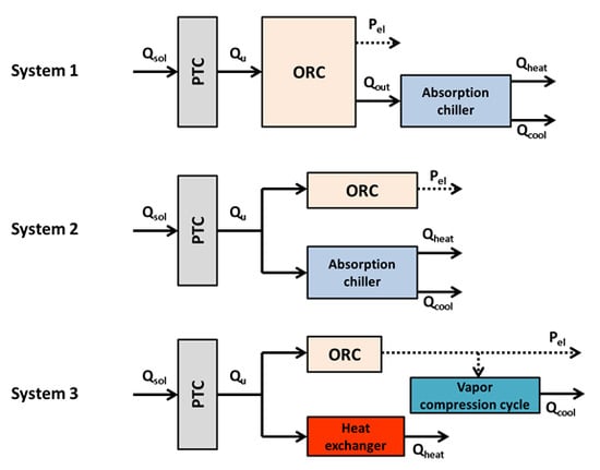
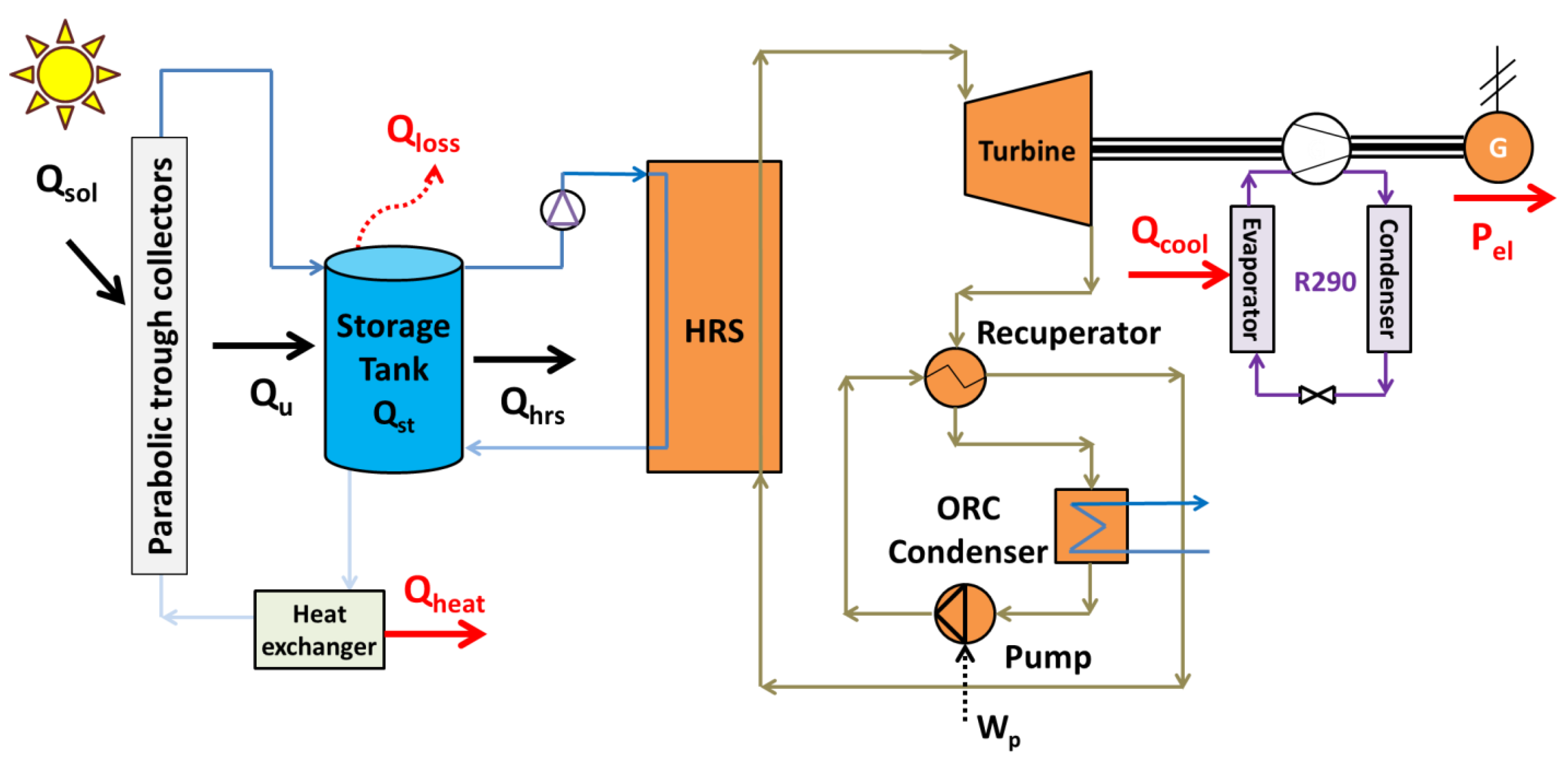
The previous literature review indicates that there is a lot of interest for solar-driven trigeneration systems and especially of systems with ORC and absorption heat pumps. So, the objective of the present work is the detailed comparison of three different versions of the trigeneration systems which combine with different ways an ORC with a heat pump. These systems can be applied in buildings with increased energy needs in order to utilize all the quantities of the produced energy rates. The comparison is energetic, exergetic and financial for presenting a multilateral analysis. The examined systems are initially optimized in steady-state conditions and their optimum designs are evaluated and compared to each other. The first system includes PTC, ORC and an ACH which is fed by the ORC’s waste heat. The second system includes PTC which feeds both ORC and ACH separately. The last system includes PTC which feeds both ORC and heating production heat exchanger separately, while the cooling is produced by a VCC which is fed by the ORC electricity production. In systems with the ACH, the heating and the cooling are both produced by this device. The yearly analysis is conducted using data for the location of Athens, Greece. The analysis is performed with developed thermodynamic models in Engineering Equation Solver (EES) [18], while the yearly analysis with a developed dynamic model in FORTRAN.

2. Materials and Methods

2.1. The Examined Systems

In this work, three solar-driven trigeneration systems are examined. These systems were driven by parabolic trough solar collectors and they are depicted in Figure 1, Figure 2 and Figure 3. All the systems produced heating, cooling and electricity. The solar field had a 100 m2 collecting area and a 4 m3 storage tank in all the cases [19]. The mass flow rate in the solar collector was 2 kg/s [20] and the working fluid was Therminol VP-1 which can operate up to 400 °C [21]. The thermal loss coefficient of the storage tank was selected at 0.5 W/m2K [22]. Table 1 includes all the previous data.
System 1 is given in Figure 1 and it includes an ORC for electricity production which feeds an ACH for cooling and heating production. The ORC has its condenser to operate at a relatively high temperature around 115–135 °C in order to give heat in the generator. The heat rejection temperature of the ORC is 5 °C greater than the generator temperature in order to have a proper heat transfer design. The heating is produced by the ACH condenser and the cooling is produced in the ACH evaporator.
System 2 includes an ORC and an ACH which are simultaneously fed by the solar field. The ORC operates in a greater temperature range in this case compared to the ORC in System 1. However, the ORC in System 2 has lower heat input compared in System 1, so there was a need for comparing these configurations.
System 3 includes an ORC and heat exchangers for heating production which are both fed by the solar field. The cooling is produced by a VCC which is driven by the shaft of the ORC turbine. So, the net electricity production of the total configuration is lower than the electricity production of the ORC.
The ORC is a regenerative cycle which operates with toluene as the working fluid. The minimum temperature difference in the recuperator is 10 °C and the pinch point in the heat recovery system (HRS) is 5 °C. The turbine isentropic efficiency was selected at 85% and the generator efficiency at 97% which are typical values. The absorption chiller operates with the working pair LiBr–H2O which produces cooling at 5 °C in the evaporator and heating at 60 °C in the condenser. The solution heat exchanger has 70% effectiveness and rejects heat to the ambient through the absorber at 40 °C. In the VCC, the working fluid is the R290 which is an environmentally friendly fluid with global warming potential close to 3. The evaporator temperature was selected at 5 °C and the condenser temperature at 40 °C in this device, while the compressor isentropic efficiency at 85%. The heat exchanger was selected to produce heating at 60 °C. Table 2 includes all the previous values.

2.2. Basic Mathematical Modeling

The main equations about the system description are given. More details can be found in the references [7,11,23] about the modeling of the various configurations. The available solar energy (Qsol) can be calculated as:
Q s o l = A c o l G b
The useful heat production of the PTC (Qu) is given as:
Q u = η t h , c o l Q s o l
The system is evaluated thermodynamically by using the energy and the exergy efficiencies. In these indexes, the three useful outputs which are used as the following: power production (Pel), cooling production (Qcool) and heating production (Qheat). The input in the system is solar energy (Qsol) in every case.
The system energy efficiency (ηen) can be written as:
η en = P e l + Q h e a t + Q c o o l Q s o l
The electricity production (Pel) is produced from the electrical generator which is coupled to the turbine shaft in all the systems. The net value of the electricity is found by reducing the electricity consumption of the motor that drives the fluid pump and reducing the work consumption of the compressor in System 3. The heating production (Qheat) is produced by the condenser in the absorption chiller in Systems 1 and 2, while in System 3, it is taken by the solar field by using a proper heat exchanger. The cooling production (Qcool) is produced by the evaporator of the absorption chiller in Systems 1 and 2, while it is produced by the VCC evaporator in System 3.
The exergy efficiency of the system (ηex) is given by using the Petela model for the exergy flow of the solar irradiation [24]. The sun temperature (Tsun) was selected at 5770 K. In addition, it has to be said that the temperature level in the following expression has to be in Kelvin units.
η ex = P e l + Q h e a t + Q c o o l Q s o l [ 1 4 3 T a m T s u n + 1 3 ( T a m T s u n ) 4 ]
The thermal efficiency of the examined solar system (ηth,col) is given by the following formulas [25]:
η th , col = 0.7408 K 0.0432 T f T a m G b 0.000503 ( T f T a m ) 2 G b
The incident angle modifier (K) is calculated according to the next expression [26]:
K ( θ ) = cos ( θ ) 5.25097 10 4 θ 2.85962 10 5 θ 2
The angle (θ) is calculated for a 1-axis tracking system with the PTC axis in the south-north direction and tracking the sun in the east-west direction [26]. Moreover, it would be important to provide a general formula about the energy balance in the storage system. The heat input in the tank is the useful heat production (Qu), while the tank gives heat in other devices (Qdevices) and there are tank thermal losses (Qloss). The remaining energy is stored in the tank (Qst) as sensible heat. The other devices are the HRS, the absorption chiller in System 2 and the heat exchanger in System 3.
Q s t = Q u Q l o s s Q d e v i c e s
In the present study, the financial evaluation of the examined systems was performed by using the simple payback period (SPP) index. This parameter shows the period in years which is needed in order for the initial investment cost to be balanced by the yearly incomes. The general expression of the (SPP) is given below:
S P P = C 0 C F
The investment cost (C0) takes into consideration the solar field cost and the trigeneration system cost. The general expression of the investment cost for all the systems is given below. In the cases that a system does not have a device, then its cost is not taken into account.
C 0 = K o r c P e l , o r c + K a c h Q c o o l + K v c c Q c o o l + K h e x + K c o l A c o l + K tan k V
The yearly income (or cash flow (CF)) takes into account the income from the electricity, cooling and heating selling. The operation and maintenance costs are also included in the SPP by reducing the yearly income. More specifically, the yearly income can be calculated as below, for the operation period (Time) which was selected at 2500 h in this work.
C F = P e l T i m e K e l + Q c o o l T i m e K c o o l + Q h e a t T i m e K h e a t K O & M

2.3. Followed Methodology

The present study was performed by using three thermodynamic models which were developed in Engineering Equation Solver (EES) [18]. These models were based on equations about the modeling of the various devices. Appendix A includes information about the ORC modeling, Appendix B about the ACH modeling and Appendix C about the VCC modeling. In every system, some typical values in critical parameters were used in order to examine representative cases of Systems 1, 2 and 3. It is important to state that in this work, the solar irradiation was selected at 700 W/m2 and the solar angle at 30°. The system was assumed to operate at about 2500 h per year. These operating conditions were equivalent to simulating the yearly performance of the system in Athens, Greece. Practically the product of the 2500 h with the 700 W/m2 gives the yearly solar beam potential in this location [27]. The solar angle of the 30° led approximately to an incident angle modifier close to its yearly mean value for this location, according to reference [26]. The ambient temperature was selected at 25 °C which is a typical value for the examined location. Table 3 summarizes all the aforementioned data for the system operation.
Firstly, the three systems were compared by performing a sensitivity analysis. The second step was the optimization of the three systems. The optimization goal is the minimization of the simple payback period because this parameter indicates the viability of the studied technologies. The optimization was conducted by using the conjugate directions method or “Powell’s method” which is supported by EES [18]. The optimization variables were the superheating in the turbine inlet (ΔTsh) which ranged from 0 °C up to 40 °C, the ACH generator temperature which ranged from 110 °C up to 130 °C and the turbine inlet pressure (or ORC high pressure). The high-pressure level in the turbine inlet was examined by using the dimensionless pressure ratio (α) which is defined as the ratio of the pressure level in the turbine inlet (Ph) to the working fluid critical pressure (Pcrit).
α = p h p c r i t
The maximum value of the parameter (α) was selected at 90% in order to avoid stability issues [28]. In this work, the range of this parameter was selected to be from 50% up to 90%. Moreover, it is important to state that the selected ranges are in accordance with the existing literature [7] and they correspond to reasonable values for safe operation.
Furthermore, the generator heat input in System 2 was selected at 15 kW, while the cooling and the heating production were selected both at 10 kW in System 3. These assumptions were performed in order for all the systems to have similar useful output productions and so the comparison to be possible.
About the financial analysis, the simple payback period (SPP) was used as the investigation criterion. The cost of the PTC was estimated at 250 €/m2 [29]. The ORC cost was selected at 3000 €/kWel, the cost of the absorption chiller at 1000 €/kWcool, the cost of the VCC at 300 €/kWcool and the cost of the storage tank at 1000 €/m3. The electricity cost was selected at 0.20 €/kWh, the heating cost at 0.10 €/kWh and the cooling cost at 0.067 €/kWh [30]. Lastly, it has to be said that the operation and maintenance cost was selected to be at 1% of the investment cost. Table 4 summarizes the used cost values in the present analysis.

3. Results and Discussion

In this section, the results of the system’s performance are given. Section 3.1 is devoted to presenting a simple sensitivity analysis of the three systems, while Section 3.2 gives the optimization procedure results.

3.1. Sensitivity Analysis of the Three Systems

The first step in this work is the sensitivity analysis of the examined system. In all the cases, only one parameter changes while the others are selected to have typical constant values. More specifically, the reference values of the parameters are 90% for the pressure ratio, 20 °C for superheating and 115 °C generator temperature.
Figure 4 and Figure 5 show the impact of the superheating in the turbine inlet on the results. Figure 4 indicates that in all the cases the SPP, System 1 is the lowest with System 2 to follow and System 3 to have the highest SPP and to be the less viable case. Generally, higher superheating is beneficial for Systems 2 and 3, while System 1 needs small or no superheating. Figure 5 shows the results of the energy and the exergy efficiency for different superheating values. Both energetically and exergetically, System 1 has the highest efficiency with System 2 to follow and System 3 to be the less efficient system. Generally, higher superheating is beneficial except for the energy efficiency of System 1.
Figure 6 and Figure 7 illustrate the impact of the pressure ratio on the system performance. System 1 has the lowest SPP for all the cases with System 2 to follow and System 3 to be the least viable case. The increase of the pressure ratio is not financially beneficial and especially it leads to a high increase of the SPP for System 1. Figure 7 depicts the results of the energy and the exergy efficiency for different pressure ratio values. The variation of this parameter is not so important for Systems 2 and 3, while it has more influence on System 1. Higher pressure ratio increases the exergy efficiency of System 1 while it reduces energy efficiency. Practically, a higher pressure ratio leads to higher electricity production due to the higher ORC efficiency, something that is beneficial for the exergy efficiency. On the other hand, lower electricity production leads to higher heat rejection from the ORC to the absorption chiller, something that increases the heating and the cooling productions which are powerfully associated with energy efficiency.
Figure 8 and Figure 9 depict the influence of the generator temperature on the results. Systems 1 and 2 are only compared because System 3 does not include an absorption chiller. Figure 8 shows that higher generator temperature reduces the SPP of both systems. Figure 9 indicates that higher generator temperature is beneficial for the energy and exergy efficiency of both systems. So, all the factors indicate that the generator temperature has to take high values. In this work, the maximum generator temperature has been selected at 130 °C in order not to have crystallization problems in the absorption chiller.

3.2. Optimization of the Three Systems

These results of this section correspond to the optimized designs in order to make a suitable comparison. Figure 10, Figure 11, Figure 12, Figure 13, Figure 14 and Figure 15 show the comparative results and Table 1 summarizes the comparison data of this work.
Figure 10 depicts the energy efficiency comparison. System 1 is the most efficient energetically with 78.17%, while System 2 follows with 43.30% and System 3 with 37.45%. These results show that the use of waste heat from the ORC condenser is more efficient than using separate ORC and ACH. The disadvantage of rejecting heat in high temperature in System 1 is not so strong and so System 1 is the best choice energetically. Figure 11 shows the exergy results which show the same performance sequence. More specifically, System 1 has 15.94% exergy efficiency, System 2 presents 13.08% and System 3 12.25%. Generally, the results of Figure 10 and Figure 11 indicate that System 1 has a greater difference than the other systems, while Systems 2 and 3 have a small but important difference.
Figure 12 gives the simple payback period of the examined systems. System 1 has the lowest simple payback period and so it is the best case financially. More specifically, the SPP of the three systems is 5.62, 7.82 and 8.49 years, respectively. It is important to state that the SPP is not so high in all the cases for a renewable energy system and so all the investments are financially viable. This is an important result which makes clear that the solar-driven trigeneration systems with PTC can be used in the future with both energetic and financial gain.
Figure 13, Figure 14 and Figure 15 illustrate the electricity, heating and cooling production of the examined configurations. It can be said that the cooling and the heating productions of System 1 are significantly higher than the respect of the other systems. Moreover, electricity production is similar to the studied units. So, it is clear that System 1 seems to be the best because it can give generally higher useful outputs than others. More specifically, the electricity production of the three systems is found at 6.05 kW, 6.39 kW and 6.21 kW, respectively. The heating production of the three systems is found at 25.28 kW, 12.42 kW and 10.00 kW, respectively. The cooling production of the three systems is found at 23.39 kW, 11.49 kW and 10.00 kW.
At this point, it has to be discussed that the generator heat inputs in System 2 and the heating/cooling productions in System 3 could have different values than those selected. However, a sensitivity analysis proved that there is not any case with adequate electricity production where these systems are better for System 1. In other words, the generator heat input in System 2 has been selected at 15 kW and the heating/cooling productions in System 3 at 10 kW. However, it has been found that these selections are not able to change the final results which indicate that the system is the overall optimum choice financially, energetically and exergetically. Table 5 includes the aforementioned values and also the values of the optimization variable parameters.
The found results indicate that the use of solar energy for producing significant amounts of electricity, heating and cooling is possible. All the trigeneration systems are efficient with System 1 to be the best choice. So, it is suggested to incorporate these systems in the building sector and especially in cases with high energy needs. Hospitals, commercial buildings and blocks of building apartments are possible kinds of buildings that can use solar-driven trigeneration systems. Moreover, it has a lot of interest to use new storage technologies with phase change materials or thermochemical storage in order to enhance the daily efficiency of the units.

4. Conclusions

The objective of the present work is the comparison of three different solar-driven trigeneration systems which are ideal for the building sector. These systems operate with parabolic trough collectors, organic Rankine cycle and heat pumps. The analysis is conducted by using developed models in Engineering Equation Solver. The comparison is energetic, exergetic and financial. The most important conclusions of this work are summarized below:
-
System 1 presents 78.17% energy efficiency, System 2 43.30% and System 3 37.45%. Thus, System 1 is the best choice energetically.
-
System 1 presents 15.94% exergy efficiency, System 2 13.08% and System 3 8.49%. These results indicate that System 1 is the best choice exergetically.
-
The simple payback period is found to be 5.62 years for System 1, 7.82 years for System 2 and 8.49 years for System 9. So, System 1 is the best choice financially.
-
The electricity production in System 1 is 6.05 kW, the heating production is 25.28 kW and the cooling production is 23.39. The heating and the cooling production of this system are higher than the other systems with a significant difference. The electricity production is similar to the other systems but it is a bit lower.
-
System 1 is found to be the optimum system according to all the criteria (SPP, energy efficiency and exergy efficiency), while System 2 is the second choice and System 3 is the last choice. However, all the systems are found to be financially viable.
Finally, it can be said that the combination of the ORC with the ACH is an intelligent idea because the waste heat of the ORC is utilized for heating and cooling production. There is a small sacrifice in the produced electricity, compared to the case with the ORC condemner to be set at a lower temperature, but this is not enough to counterbalance the overall gain with the design of System 1. Moreover, it has to be highlighted that the examined systems can easily be applied in buildings with high energy needs such as hospitals, commercial buildings and blocks of apartments with central heating/cooling systems.

Author Contributions

C.T. supervision, writing—review and editing, writing—original draft preparation; E.B. conceptualization, methodology, investigation, writing—review and editing, writing—original draft preparation. All authors have read and agreed to the published version of the manuscript.

Funding

This research is co-financed by Greece and the European Union (European Social Fund ESF) through the Operational Programme, Human Resources Development, Education and Lifelong Learning, in the context of the project “Reinforcement of Postdoctoral Researchers 2nd Cycle” (MIS-5033021), implemented by the State Scholarships Foundation (IKΥ).

Acknowledgments

Evangelos Bellos would like to thanks the State Scholarships Foundation (IKΥ) for its financial support (MIS-5033021).
Energies 13 02074 i001

Conflicts of Interest

The authors declare no conflicts of interest.

Nomenclature

AcolCollecting area, m2
C0Capital cost, €
CFYearly cash flow income, €
GbSolar direct beam irradiation, W/m2
hSpecific enthalpy, kJ/kg
KIncident angle modifier, -
KachSpecific cost of the absorption chiller, €/kWcool
KcolSpecific cost of the collector, €/m2
KelElectricity cost, €/kWhel
KcoolCooling cost, €/kWhcool
KheatHeating cost, €/kWhheat
KhexCost of the heat exchanger for heating production, €
KorcSpecific cost of the organic Rankine cycle, €/kWel
KO&MYearly cost for operation and maintenance, €
KtankSpecific cost of the storage tank, €/m3
mMass flow rate, kg/s
mrRefrigerant Mass flow rate, kg/s
pcritCritical pressure of the working fluid, bar
phPressure in the turbine inlet, bar
PelElectricity production, kWel
QHeat rate, kW
SPPSimple Payback Period, years
TTemperature, °C
TimeYearly operating period of the system, h
VStorage tank volume, m3
WpElectricity consumption of the pump motor, kW
WTTurbine work production, kW
XLiBr mass concentration, %
Greek Symbols
αRatio of the turbine inlet pressure to the critical pressure, -
ΔPPressure increase in the heat pump, bar
ηEfficiency, -
ηgElectrical generator efficiency, -
ηhexSolution heat exchanger efficiency, -
ηmMechanical efficiency, -
ηmotorMotor efficiency, -
θIncident solar angle, °
ρDensity, kg/m3
Subscripts and Superscripts
amAmbient
cCondenser of the absorption chiller
colCollector
comCompressor
condCondenser of the vapor compression cycle
coolCooling production
devicesDevices of the total system
elElectricity production
enEnergy
exExergy
fFluid
heatHeating production
isIsentropic
lossTank losses
orcOrganic Rankine cycle
solSolar
stStorage
strStrong
sunSun
TTurbine
thThermal
uUseful
wWeak
Abbreviations
ACHAbsorption Chiller
EESEngineering Equation Solver
HRSHeat Recovery System
ORCOrganic Rankine Cycle
PTCParabolic Trough Collector
VCCVapor Compression Cycle

Appendix A. Basic Modeling of the Organic Rankine Cycle

Appendix A is devoted to presenting the basic equations for the modeling of the ORC. Figure A1 shows the basic depiction of a regenerative ORC.
Figure A1. The basic regenerative organic Rankine cycle.
Energies 13 02074 g0a1
The work production (WT) of the turbine is calculated as below:
W T = m ( h 4 h 5 )
The isentropic efficiency of the turbine (ηis,T) is defined as:
η is , T = h 4 h 5 h 4 h 5 , i s
In this work, the isentropic efficiency of the turbine was selected at 85% which is a typical value.
The electricity consumption of the pump motor (WP) is calculated as:
W p = m Δ P ρ η motor
The energy balance in the recuperator can be written as below:
h 5 h 6 = h 3 h 2
The net electricity production (Pel) for Systems 1 and 2 can be written as below:
P el = η g η m W T W p
The net electricity production for System 3 has to take into consideration the work demand of the compressor (Qcom) and so the following expression can be written:
P el = η g ( η m W T W c o m η m ) W p

Appendix B. Basic Modeling of the Absorption Chiller

Appendix B is devoted to presenting the basic equations for the modeling of the ACH. Figure A2 shows the basic depiction of the ACH with a solution heat exchanger.
Figure A2. The basic depiction of the absorption chiller operating with the LiBr–H2O working pair.
Energies 13 02074 g0a2
The cooling production in the evaporator (Qcool) is calculated as:
Q c o o l = m r ( h j h i )
The energy balance in the generator can be written as below:
Q g = m r h g + m s t r h d m w h c
The energy balance in the absorber can be written as below:
Q a = m r h j + m s t r h f m w h a
The heating production (Qheat) can be written as below:
Q h e a t = Q c = m r ( h g h h )
The heat exchanger effectiveness (ηhex) is defined a below:
η = h d h e h d h b
In this work, the heat exchanger effectiveness was selected at 70% which is a reasonable value.
The energy balance in the solution heat exchanger can be written as below:
m w ( h c h b ) = m s t r ( h d h e )
The work in the solution pump is negligible and thus it can be said:
h b = h a
The processes in the throttling valves are ideal and thus the enthalpy levels did not change:
h f = h e
h i = h h
The total mass flow rate balance in the absorber can be written as:
m w = m s t r + m r
The LiBr substance mass flow rate balance in the absorber can be written as:
X w m w = X s t r m s t r
Moreover, it is important to state that the state point “j” is assumed to be saturated steam and the state point “h” to be saturated water.

Appendix C. Basic Modeling of the Vapor Compression Cycle

Appendix C is devoted to presenting the basic equations for the modeling of the VCC. Figure A3 shows the basic depiction of the examined VCC.
Figure A3. The basic vapor compression cycle of this work.
Energies 13 02074 g0a3
The work demand in the compressor (Wcom) is calculated as:
W c o m = m r ( h 2 h 1 )
The isentropic efficiency of the compressor (ηis,com) is defined as:
η is , com = h 2 , i s h 1 h 2 h 1
Moreover, it has to be said that in this work, the isentropic efficiency of the compressor was selected at 85% which is a typical value.
The cooling production (Qcool) is calculated as below:
Q c o o l = m r ( h 1 h 4 )
The heat rejection from the condenser to the ambient (Qcond) is calculated as below:
Q c o n d = m r ( h 3 h 2 )

References

  1. Wang, F.; Cheng, Z.; Tan, J.; Yuan, Y.; Shuai, Y.; Liu, L. Progress in concentrated solar power technology with parabolic trough collector system: A comprehensive review. Renew. Sustain. Energy Rev. 2017, 79, 1314–1328. [Google Scholar] [CrossRef]
  2. Bellos, E.; Tzivanidis, C. Alternative designs of parabolic trough solar collectors. Prog. Energy Combust. Sci. 2019, 71, 81–117. [Google Scholar] [CrossRef]
  3. Zhang, M.; Ge, X.; Zhao, Y.; Xia-Bauer, C. Creating statistics for China’s building energy consumption using an adapted energy balance shee. Energies 2019, 12, 4293. [Google Scholar] [CrossRef] [Green Version]
  4. Kasaeian, A.; Nouri, G.; Ranjbaran, P.; Wen, D. Solar collectors and photovoltaics as combined heat and power systems: A critical review. Energy Convers. Manag. 2018, 156, 688–705. [Google Scholar] [CrossRef] [Green Version]
  5. Wu, D.W.; Wang, R.Z. Combined cooling, heating and power: A review. Prog. Energy Combust. Sci. 2006, 32, 459–495. [Google Scholar] [CrossRef]
  6. Al-Sulaiman, F.A.; Dincer, I.; Hamdullahpur, F. Exergy modeling of a new solar driven trigeneration system. Sol. Energy 2011, 85, 2228–2243. [Google Scholar] [CrossRef]
  7. Bellos, E.; Tzivanidis, C. Parametric analysis and optimization of a solar driven trigeneration system based on ORC and absorption heat pump. J. Clean. Prod. 2017, 161, 493–509. [Google Scholar] [CrossRef]
  8. Eisavi, B.; Khalilarya, S.; Chitsaz, A.; Rosen, M.A. Thermodynamic analysis of a novel combined cooling, heating and power system driven by solar energy. Appl. Therm. Eng. 2018, 129, 1219–1229. [Google Scholar] [CrossRef]
  9. Zhao, L.; Zhang, Y.; Deng, S.; Ni, J.; Xu, W.; Ma, M.; Lin, S.; Yu, Z. Solar driven ORC-based CCHP: Comparative performance analysis between sequential and parallel system configurations. Appl. Therm. Eng. 2018, 131, 697–706. [Google Scholar] [CrossRef]
  10. Khalid, F.; Dincer, I.; Rosen, M.A. Techno-economic assessment of a renewable energy based integrated multigeneration system for green buildings. Appl. Therm. Eng. 2016, 99, 1286–1294. [Google Scholar] [CrossRef]
  11. Bellos, E.; Vellios, L.; Theodosiou, I.C.; Tzivanidis, C. Investigation of a solar-biomass polygeneration system. Energy Convers. Manag. 2018, 173, 283–295. [Google Scholar] [CrossRef]
  12. Mathkor, R.Z.; Agnew, B.; Al-Weshahi, M.A.; Latrsh, F. Exergetic Analysis of an Integrated Tri-Generation Organic Rankine Cycle. Energies 2015, 8, 8835–8856. [Google Scholar] [CrossRef]
  13. Zhang, Y.; Deng, S.; Zhao, L.; Ni, J.; Ma, M.; Lin, S.; Zhang, Z. Clarifying the bifurcation point on Design: A Comparative Analysis between Solar-ORC and ORC-based Solar-CCHP. Energy Procedia 2017, 142, 1119–1126. [Google Scholar] [CrossRef]
  14. Dabwan, Y.N.; Gang, P.; Li, J.; Gao, G.; Feng, J. Development and assessment of integrating parabolic trough collectors with gas turbine trigeneration system for producing electricity, chilled water, and freshwater. Energy 2018, 162, 364–379. [Google Scholar] [CrossRef]
  15. Wang, J.; Wu, J.; Xu, Z.; Li, M. Thermodynamic performance analysis of a fuel cell trigeneration system integrated with solar-assisted methanol reforming. Energy Convers. Manag. 2017, 150, 81–89. [Google Scholar] [CrossRef]
  16. Ozlu, S.; Dincer, I. Performance assessment of a new solar energy-based multigeneration system. Energy 2016, 112, 164–178. [Google Scholar] [CrossRef]
  17. Mata-Torres, C.; Escobar, R.A.; Cardemil, J.M.; Simsek, Y.; Matute, J.A. Solar polygeneration for electricity production and desalination: Case studies in Venezuela and northern Chile. Renew. Energy 2017, 101, 387–398. [Google Scholar] [CrossRef]
  18. F-Chart Software, Engineering Equation Solver (EES). 2015. Available online: http://www.fchart.com/ees (accessed on 15 January 2020).
  19. Bellos, E.; Tzivanidis, C.; Antonopoulos, K.A. Exergetic, energetic and financial evaluation of a solar driven absorption cooling system with various collector types. Appl. Therm. Eng. 2016, 102, 749–759. [Google Scholar] [CrossRef]
  20. Duffie, J.A.; Beckman, W.A. Solar Engineering of Thermal Processes, 2nd ed.; John Wiley & Sons Inc.: New York, NY, USA, 1991. [Google Scholar]
  21. Available online: https://www.therminol.com/products/Therminol-VP1 (accessed on 15 January 2020).
  22. Bellos, E.; Tzivanidis, C. Performance analysis and optimization of an absorption chiller driven by nanofluid based solar flat plate collector. J. Clean. Prod. 2018, 174, 256–272. [Google Scholar] [CrossRef]
  23. Bellos, E.; Skaltsas, I.; Pliakos, O.; Tzivanidis, C. Energy and financial investigation of a cogeneration system based on linear Fresnel reflectors. Energy Convers. Manag. 2019, 198, 111821. [Google Scholar] [CrossRef]
  24. Petela, R. Exergy of undiluted thermal radiation. Sol. Energy 2003, 74, 469–488. [Google Scholar] [CrossRef]
  25. EU. EuroTrough II: Extension, Test and Qualification of EUROTROUGH from 4 to 6 Segments at Plataforma Solar de Almeria; Project Cooordinator: Instalaciones Inabensa, S.A. April 2003; EU: Brussels, Belgium, 2003. [Google Scholar]
  26. Bellos, E.; Tzivanidis, C. Assessment of linear solar concentrating technologies for Greek climate. Energy Convers. Manag. 2018, 171, 1502–1513. [Google Scholar] [CrossRef]
  27. Kouremenos, D.A.; Antonopoulos, K.A.; Domazakis, E.S. Solar radiation correlations for the Athens, Greece, area. Sol. Energy 1985, 35, 259–269. [Google Scholar] [CrossRef]
  28. Tzivanidis, C.; Bellos, E.; Antonopoulos, K.A. Energetic and financial investigation of a stand-alone solar-thermal Organic Rankine Cycle power plant. Energy Convers. Manag. 2016, 126, 421–433. [Google Scholar] [CrossRef]
  29. Bellos, E.; Tzivanidis, C.; Torosian, K. Energetic, exergetic and financial evaluation of a solar driven trigeneration system. Therm. Sci. Eng. Prog. 2018, 7, 99–106. [Google Scholar] [CrossRef]
  30. Bellos, E.; Pavlovic, S.; Stefanovic, V.; Tzivanidis, C.; Nakomcic-Smaradgakis, B.B. Parametric analysis and yearly performance of a trigeneration system driven by solar-dish collectors. Int. J. Energy Res. 2019, 43, 1534–1536. [Google Scholar] [CrossRef]
Figure 1. System 1—The ORC feeds the ACH with heat.
Energies 13 02074 g001
Figure 2. System 2—The ORC and the ACH are fed separately by the solar field.
Energies 13 02074 g002
Figure 3. System 3—The ORC is fed with electricity the VCC.
Energies 13 02074 g003
Figure 4. Simple payback period for the three systems with different values of the superheating in the turbine inlet.
Energies 13 02074 g004
Figure 5. Energy and exergy efficiency for the three systems with different values of the superheating in the turbine inlet.
Energies 13 02074 g005
Figure 6. Simple payback period for the three systems with different values of the pressure ratio parameter.
Energies 13 02074 g006
Figure 7. Energy and exergy efficiency for the three systems with different values of the pressure ratio parameter.
Energies 13 02074 g007
Figure 8. Simple payback period for the three systems with different values of the generator temperature level.
Energies 13 02074 g008
Figure 9. Energy and exergy efficiency for the three systems with different values of the generator temperature level.
Energies 13 02074 g009
Figure 10. Energy efficiency of the examined systems.
Energies 13 02074 g010
Figure 11. Exergy efficiency of the examined systems.
Energies 13 02074 g011
Figure 12. Simple payback period of the examined systems.
Energies 13 02074 g012
Figure 13. Electricity production of the examined systems.
Energies 13 02074 g013
Figure 14. Heating production of the examined systems.
Energies 13 02074 g014
Figure 15. Cooling production of the examined systems.
Energies 13 02074 g015
Table 1. Data of the solar field/storage system.
ParameterValue/Description
Collector typePTC
Collecting area100 m2
Storage tank volume4 m3
Tank thermal loss coefficient0.5 W/m2K
Solar field flow rate2 kg/s
Thermal oilTherminol VP-1
Maximum oil temperature400 °C
Table 2. Main data of the examined devices in the trigeneration systems.
ParameterValue/Description
Organic Rankine Cycle (ORC)
ORC working fluidToluene
Turbine isentropic efficiency85%
Power generator efficiency97%
Temperature difference in the recuperator10 °C
Pinch point in the heat recovery system5 °C
Superheating in the turbine inlet range0–40 °C
Absorption Chiller (ACH)
ACH working pairLiBr–H2O
ACH cooling temperature5 °C
ACH heat exchanger effectiveness70%
ACH heat rejection temperature40 °C
Vapor Compression Cycle (VCC)
VCC working fluidR290
VCC heat rejection temperature40 °C
Compressor isentropic efficiency85%
VCC cooling temperature5 °C
Heating Heat Exchanger
Working fluidTherminol VP-1
Heating temperature level60 °C
Table 3. Input data for the yearly system operation.
ParameterValue
Nominal solar irradiation700 W/m2
Nominal solar angle30°
Nominal ambient temperature25 °C
Yearly operating period2500 h
Table 4. Financial data of the present analysis [29,30].
ParameterValue
PTC specific cost250 €/m2
ORC specific cost3000 €/kWel
ACH specific cost1000 €/kWcool
VCC specific cost300 €/kWcool
Storage tank specific cost1000 €/m3
Electricity price0.20 €/kWh
Heating price0.10 €/kWh
Cooling price0.067 €/kWh
Operation and maintenance cost1% ∙ C0
Table 5. Summary of the final results for the examined systems.
SystemsηenηexSPPPelQheatQcoolαΔTshTg
(-)(-)(Years)(kW)(kW)(kW)(-)(°C)(°C)
System 178.17%15.94%5.626.0525.2823.3950.0%0.0130
System 243.30%13.08%7.826.3912.4211.4958.8%27.8130
System 337.45%12.25%8.496.2110.0010.0072.1%40.0-

