Investigation of Vortical Structures and Turbulence Characteristics in Corner Separation in an Axial Compressor Stator Using DDES

Abstract

In order to investigate the flow structure and unsteady behavior of three-dimensional corner separation, a delayed detached-eddy simulation (DDES) method based on the Spalart–Allmaras (SA) model is performed on the third-stage stator of a multistage low-speed axial compressor. The stator simulation is validated by experiments before flow mechanism analysis. The complicated flow fields in the stator are then described step by step. Firstly, the structure and development process of vortices in corner separation flow are analyzed. Secondly, the velocity histogram of the monitor points in the mainstream and corner separation regions is obtained, and the velocity distribution of the corner separation region is discussed. Finally, Reynolds stress, Lumley anisotropy, turbulence energy spectra, and helicity density are discussed to understand the turbulence behavior of the corner separation flow in the stator. The results show that the corner separation appears at even the design condition and different kinds of vortical structures appear in the stator hub corner. The unsteadiness of corner separation flow is mainly reflected in the separation on the suction side of the blade and the wake shedding. Turbulence anisotropy and energy backscatter are found to be dominant in the separation region, which is correlated to the high shear stress.

1. Introduction

Three-dimensional separations are an inherent flow feature in the axial compressor corner, formed by the suction surface and the endwall. Its effect will limit the loading and reduce compressor efficiency [1,2,3]. With the change of compressor operating conditions, corner separation may develop into corner stall, causing severe passage blockage and sharp increase in losses, which adversely affects compressor stability [4]. The flow in the corner region is highly unsteady and vortical; considering the high cost and limitations of unsteady flow test measurement, it is an effective method to obtain three-dimensional unsteady flow, and reveal the flow separation mechanism in the compressor corner, by using high-fidelity numerical simulation combined with corresponding experimental verification. In recent decades, a turbulence model based on Reynolds-averaged Navier–Stokes equations (RANS) has been widely used in industrial computational fluid dynamics (CFD) code [5,6,7], but the turbulence in the corner separation region has high anisotropy and non-equilibrium characteristics due to the existence of active turbulence fluctuation. Therefore, it is difficult to use RANS modeling to predict corner separation flow.

Despite the rapid development of computer power, high-fidelity numerical methods such as DNS and large eddy simulation (LES) have not been applied to complex engineering problems, mainly because of the huge computational cost [8]. The hybrid RANS/LES method uses LES to solve large-scale unsteady motion and RANS to solve steady flow [9], so it takes less computing time than genuine LES and can be applied to solve engineering turbulence problems. The hybrid RANS/LES method has recently been applied to investigate vortex structures, unsteady mechanisms, and turbulence characteristics of corner separation in compressor cascades. Wang et al. found that the unsteadiness of the corner region was caused by the suction surface separation and the wake shedding [10], while Xia et al. believed that the dynamics of the horseshoe was the main contribution to the unsteadiness in the corner separation [11]. Xia et al. also emphasized that horseshoe vortex played a key role in corner separation, whereas in Liu et al.’s [12], the passage vortex enhanced the corner separation in the compressor cascade.

At present, the understanding of the vortex structures of corner separation and the main sources of unsteadiness is still immature. Moreover, previous studies mainly focus on the linear cascades; there exist differences in blade geometry and inlet flow conditions between the linear cascade and the real compressor stator, for instance, 3D blade stacking may alter the behavior of the corner separation [13]. Considering these factors, the third stage stator of a multistage low-speed axial flow compressor is taken as the research object in this paper, and the delayed detached eddy simulation (DDES) method is used to explore the vortex structure, unsteadiness, and turbulence characteristics of the three-dimensional corner separation of the compressor stator at the design operating condition.

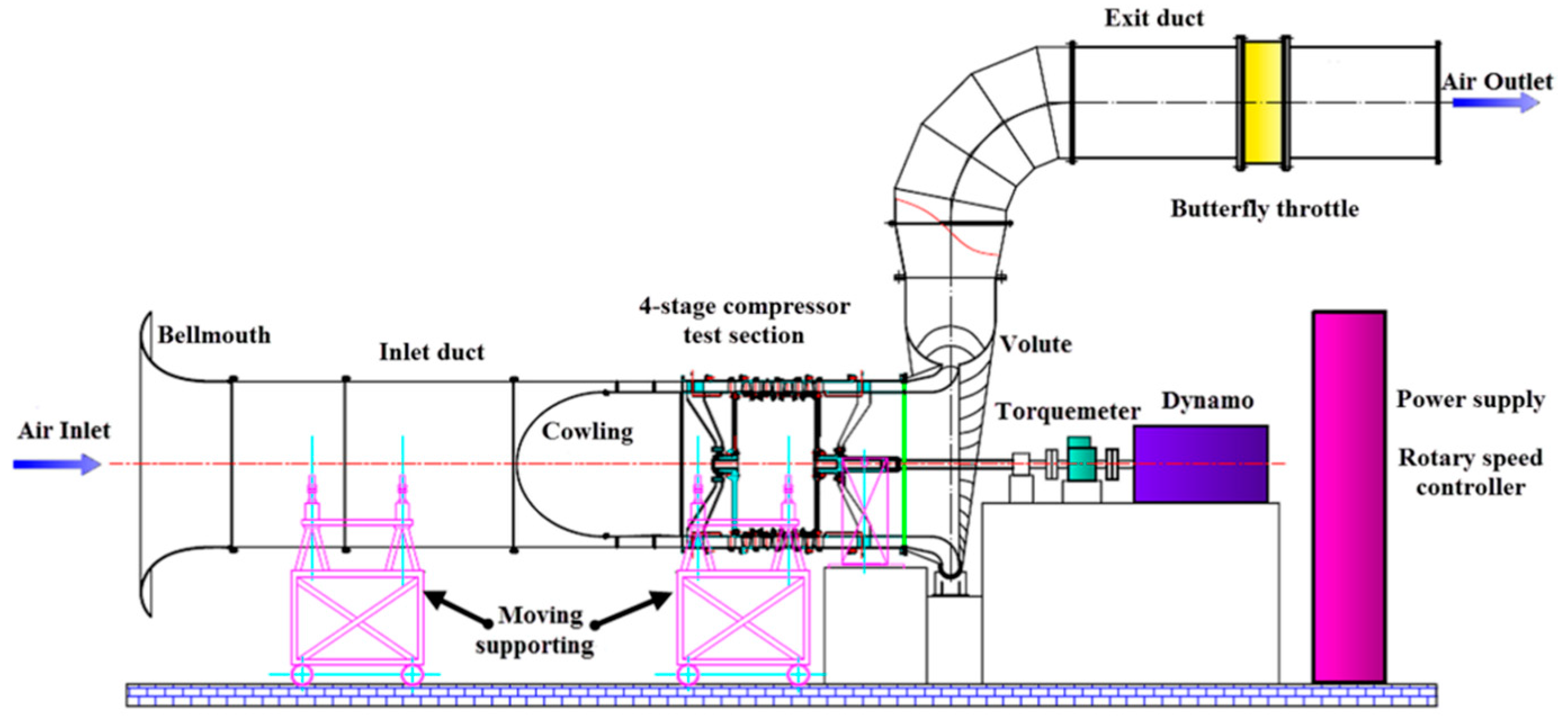
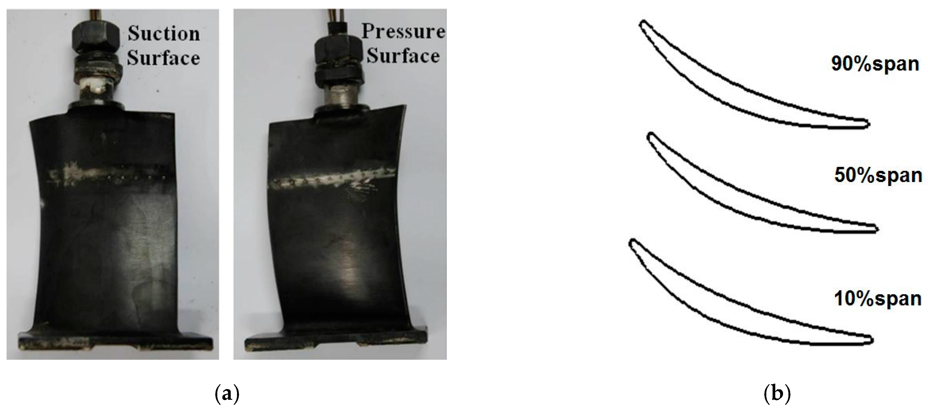
2. Low-Speed Research Stator

The object of this research is the third-stage stator of the four-stage low-speed axial compressor, which is used for the low-speed model testing at Nanjing University of Aeronautics and Astronautics [14,15,16]. The low-speed test rig mainly includes bell-mouth, inlet and exit ducts, cowling, 4-stage large-scale compressor test section, air-exhaust volute, butterfly throttle, driven dynamo, and moving supporting, as shown in Figure 1. Figure 2 shows a pictorial view of the stator blade and profile configurations at three typical blade spans. General specifications of the low-speed axial compressor stator are listed in

Table 1. General specifications of the low-speed axial compressor stator.

Design Parameter	Value
Blade number	120
Casing diameter (mm)	1500
Hub-to-tip ratio	0.88
Mid-span Reynolds Number	4.6 × 105
Chord (tip/mid/hub) (mm)	61.0/60/64.8
Solidity (tip/mid/hub)	1.61/1.64/1.91
Mass flow rate coefficient	0.385
Tip clearance/blade height (%)	0

. Geometric parameters of the stator are listed in

Table 2. Geometric parameters of the stator.

r/R	Chord (mm)	Stagger Angle γ (°)	Leading Blade Angle α1k (°)	Trailing Blade Angle α2k (°)	Maximum Relative Thickness Cmax
0.00	61.0	54.82	61.71	−0.25	0.0795
0.05	61.1	52.53	61.14	0.42	0.0791
0.10	60.2	51.43	60.65	1.17	0.0861
0.30	59.7	51.61	59.74	2.28	0.0822
0.50	60.0	51.48	59.87	2.89	0.0820
0.70	60.9	51.57	60.99	2.64	0.0848
0.90	63.5	52.14	63.57	1.65	0.0969
0.95	64.2	53.43	64.23	1.20	0.1020
1.00	64.8	53.82	64.85	0.24	0.1066

. In addition, the stator lean and leading and trailing metal angle are presented in Figure 3a.

To validate the simulation, the four-hole probe was designed to measure the inlet and outlet flow field of the research stator, because the axial gap size between adjacent rows is small, and it is impossible to measure with a five-hole pneumatic probe. Details of calibration procedures and results for multi-hole pneumatic probes can be found in [17]. The pneumatic four-hole probe was traversed by a 3-DOF displacement mechanism (shown in Figure 3b) in the compressor test, and the precision of the mechanism was within ± 0.1 mm and ± 0.1°. Detailed area traverses of upstream and downstream of the stator using pneumatic four-hole probe were conducted at the design operating condition. All measuring planes are located in the middle of the axial gap. The traverse was performed on one stator pitch and from 8% to 99% span. Seventeen and nineteen points were arranged along the pitch and span, respectively.

3. Computational Procedure

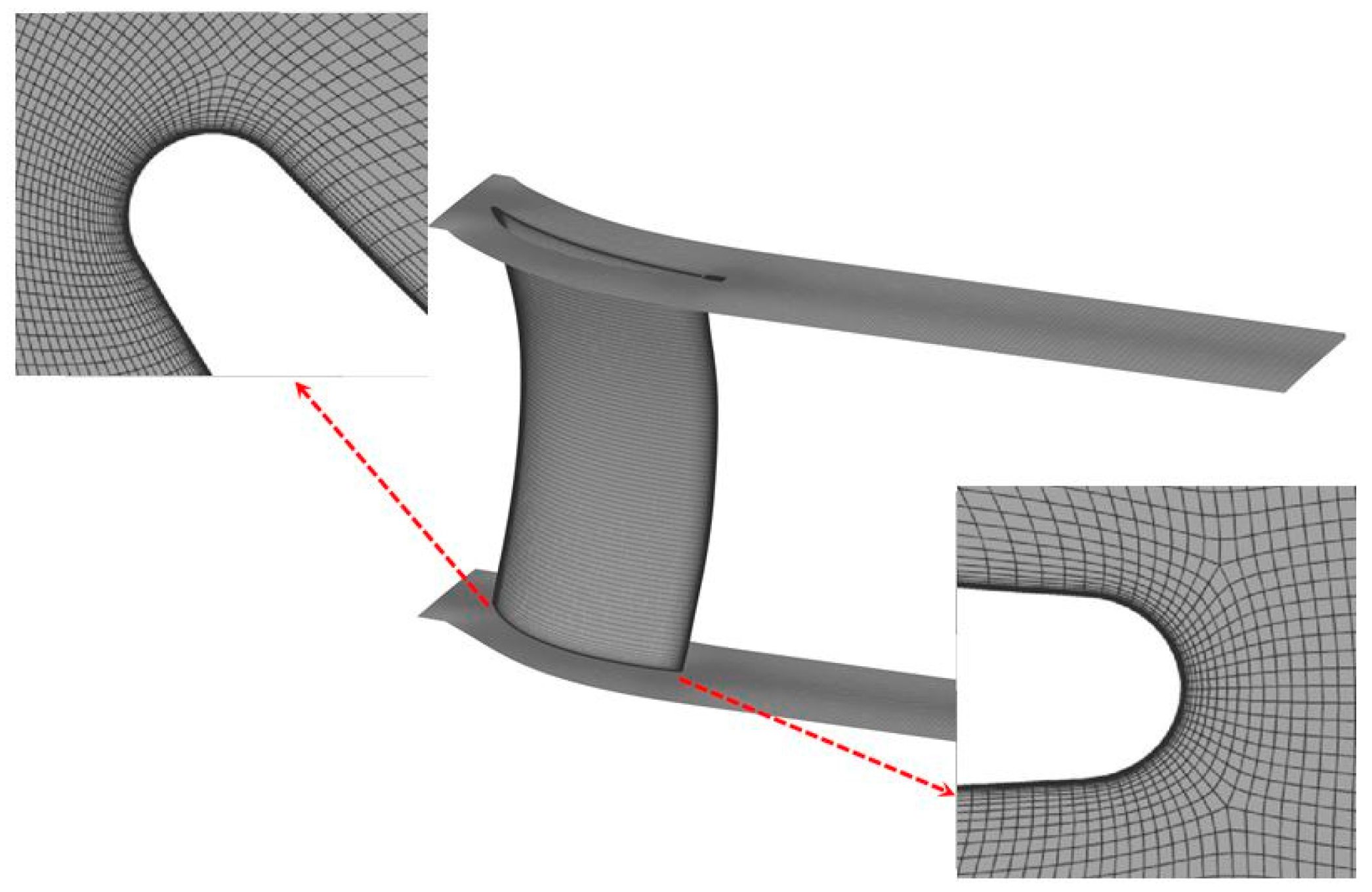
3.1. Computational Grids

The single-passage configuration of the research stator was selected as the computational zone. As shown in Figure 4, hexahedral structured meshes were generated in O4H topology to model the mainflow region, in order to reduce the mesh skewness. The mainflow region of the stator was divided into five blocks, and the node distributions of five parts were: 77 × 121 × 305; 17 × 121 × 65; 17 × 121 × 121; 77 × 121 × 305; and 17 × 121 × 273, along the circumferential, radial, and axial directions, respectively. The grid scale based on the chord in the spanwise, pitchwise, and streamwise was ∆x/c < 0.0123, ∆y/c < 0.0072, and ∆z/c < 0.0069, respectively. The height of the first grid cell to the solid wall was 3 × 10⁻⁶ m, which ensured y⁺ < 1 at the wall. The final mesh size of the computational domain reached about 7.0 million.

3.2. Boundary Conditions

No-slip and no-heat transfer conditions were imposed at solid boundaries. In addition, periodic boundary conditions were set along the circumferential direction. The inlet plane was located 0.24c upstream of the blade leading edge, which seems shorter than the common knowledge. In fact, previous research results have shown that, due to the development of the endwall boundary layer, the relatively long upstream extension domain cannot guarantee the inlet boundary layer [18], so the computation was performed with relatively short inlet length, where its inlet plan was the measurement position used in the previous experiments. The spanwise distributions of the total pressure, total temperature, and flow angle obtained by reliable experiments were arranged for inlet plan. The outlet plane was located 2.4 chord downstream of the blade trailing edge. At the outlet plan, static pressure at the mid-span was imposed. Figure 5 shows the radial distribution of total temperature, flow angle, and velocity obtained from the experiment at the stator inlet.

3.3. Numerical Method

The DDES is a type of hybrid RANS/LES method, which narrows the gray scale region between RANS and LES and ensures that the LES model is not used in the boundary layer region. In order to better explore the development of vortices in corner separation, the DDES method based on the Spalart–Allmaras (SA) model was used in this paper. The SA model equation is defined as follows:

$$\frac{\partial }{\partial t}\left(\rho \tilde{\nu }\right)+\frac{\partial }{\partial x_i}\left(\rho \tilde{\nu }{u}_i\right)=c_{b1}\rho \tilde{S}\tilde{\nu }+\frac{1}{{\sigma }_{\tilde{\nu }}}\left\{\frac{\partial }{\partial x_j}\left[\left(\mu +\rho \tilde{\nu }\right)\frac{\partial \tilde{\nu }}{\partial x_j}\right]+c_{b2}\rho {\left(\frac{\partial \tilde{\nu }}{\partial x_j}\right)}^2\right\}-c_{w1}\rho f_w{\left(\frac{\tilde{\nu }}{d}\right)}^2$$

(1)

where d represents the distance from the grid point to the nearest wall in the equation. The model switching from the RANS to the LES in the calculation depends on the new $\tilde{d}$, which is expressed as follows:

$$\tilde{d}=d-f_d\max \left(0,d-C_{des}\Delta \right)$$

(2)

$$f_d=1-\tanh \left({(8r_d)}^3\right)$$

(3)

$$r_d=\frac{{\nu }_t+\nu }{\sqrt{U_{ij}{U}_{ij}}{\kappa }^2{d}^2}$$

(4)

where ∆ is the grid unit scale. In the mainstream region, when d ≫ C_des∆, the LES method is activated. In the near-wall region, the method selection depends not only on the mesh, but also on the eddy viscosity. When d > C_des∆ in the near-wall region, as long as function f_d indicates that the current grid point is inside the boundary layer according to the value of r_d, the LES method is not adopted. A detailed description of the DDES-SA model can be referred [19].

In this paper, commercial software FLUENT 14.5 was used to make numerical simulation. For unsteady calculation, the pressure-based implicit solver was chosen. The second order upwind scheme and the central-differencing scheme were used for the convection terms and viscous terms of the governing equations, respectively. The average grid scale of the calculation model was about ∆ = 5.0 × 10⁻⁴ m, so the outer iteration physical time step chose 5 × 10⁻⁵ s, and 6000 time steps were performed. The corresponding total simulation time was 0.3 s.

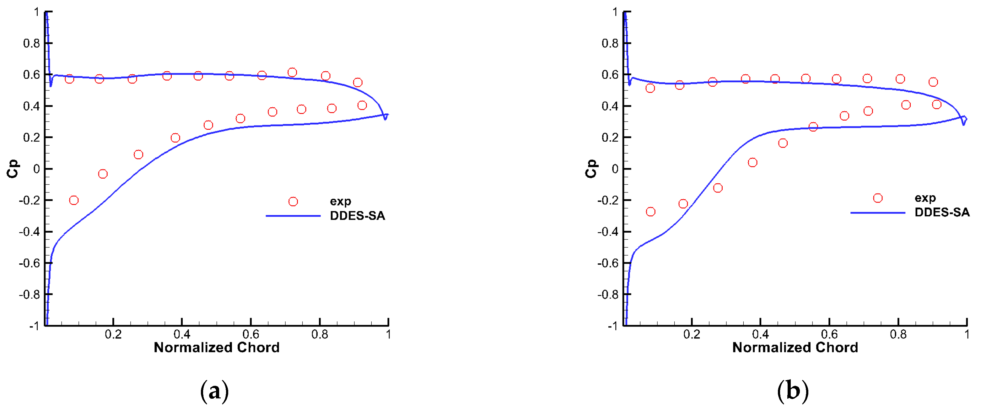
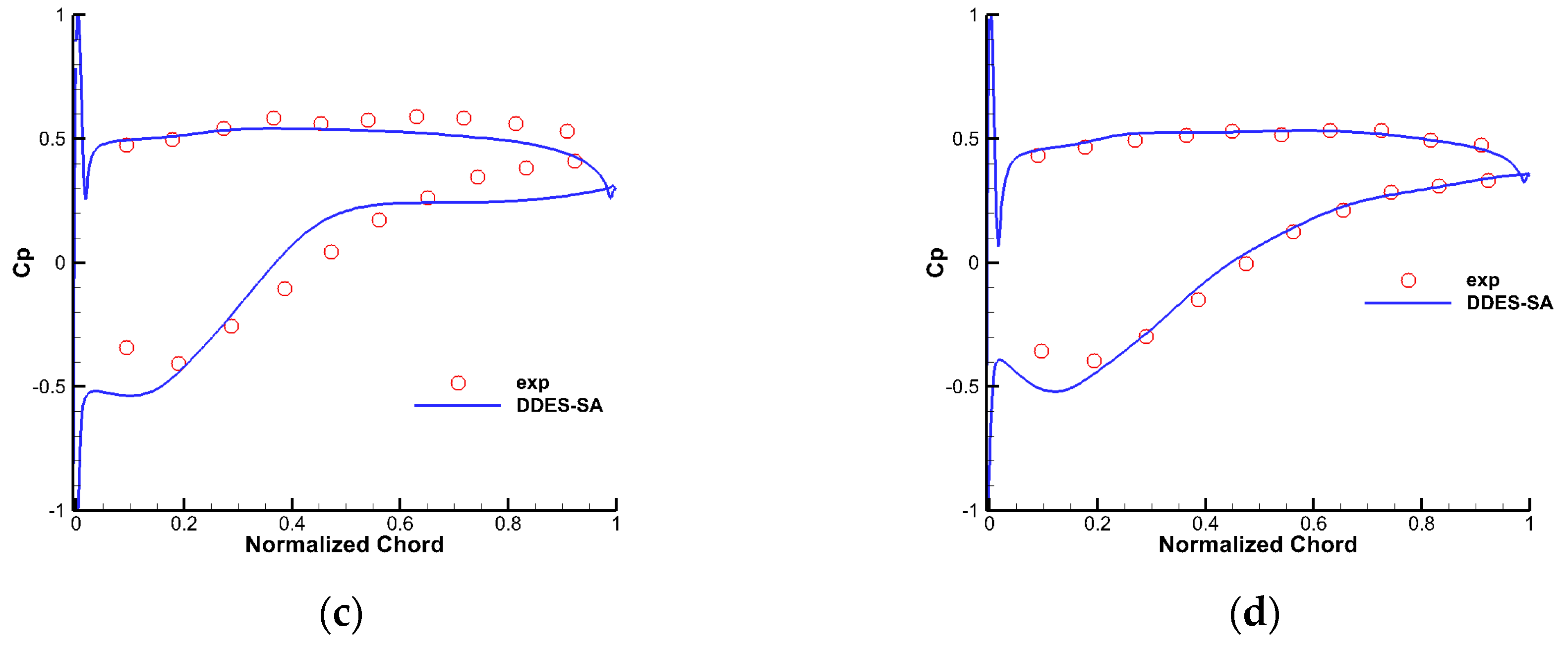
4. Validation of Numerical Results

Through the comparative analysis of the static pressure distribution along the blade surface, the total pressure loss, and the outlet flow angle, it can be verified whether the numerical calculation can simulate the real flow field in the experiment. Because the experimental data were measured by steady pressure sensors, the numerical results were averaged over time. Figure 6a indicates that the result of DDES-SA agrees with the experimental value at 70% span, because the flow is approximated as a two-dimensional flow. As shown in Figure 6b,c, the results of DDES-SA are different from the experiment at 30% and 50% span. DDES has a pressure platform at the position of 55% chord, while the experimental position is relatively backward, which shows that the DDES-SA predicts larger corner separation and earlier boundary separation than the experiment. Figure 6d shows the result of DDES-SA is consistent with the experimental results at 10% span, where the flow separation occurs at the trailing edge of the blade.

Figure 7 shows the spanwise distribution of the mass-average total pressure loss coefficient and outflow angle. The mass-averaging plane is located 0.23 chord downstream of the blade trailing edge. By comparison with the experiment, the DDES-SA method can give reasonable loss distribution from 20% to 70% span. From Figure 7a, the experimental result shows that the total pressure loss coefficient is greater at 20% to 40% span under the influence of corner separation flow. The separation position is different from the conventional corner separation of the compressor cascade because the stator hub has a certain degree of “lean”, which makes the low-energy fluid at the hub migrate upward. At 40% span, the vortices at the corner position predicted by the DDES-SA method are larger than the experiment, which results in the deviation between the DDES and the experimental value on the loss coefficient. The influence factor that the loss coefficient of DDES is lower than the experimental value at two endwalls is that the experimental value is the measurement result under the multistage environment, so the effect of the upstream and downstream rotor blade rows on the stator cannot be considered in numerical simulation. The tip leakage flow from the upstream rotor increases the loss above 80% span; at the same time, the unsteady effect from the downstream rotor flow separation increases the loss below 20% span. The distribution of exit flow angles indicates this DDES-SA method is reasonable for predicting corner separation flow, as shown in Figure 7b. Although there is a certain deviation between the numerical simulation results and the experimental values, the capture of three-dimensional corner separation is reliable, and the reliability of DES in this aspect can further explore the vortex structure and turbulence characteristics of corner separation in the compressor stator.

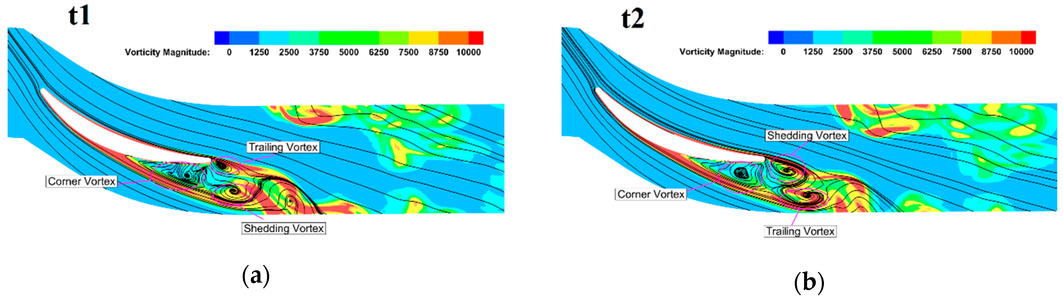
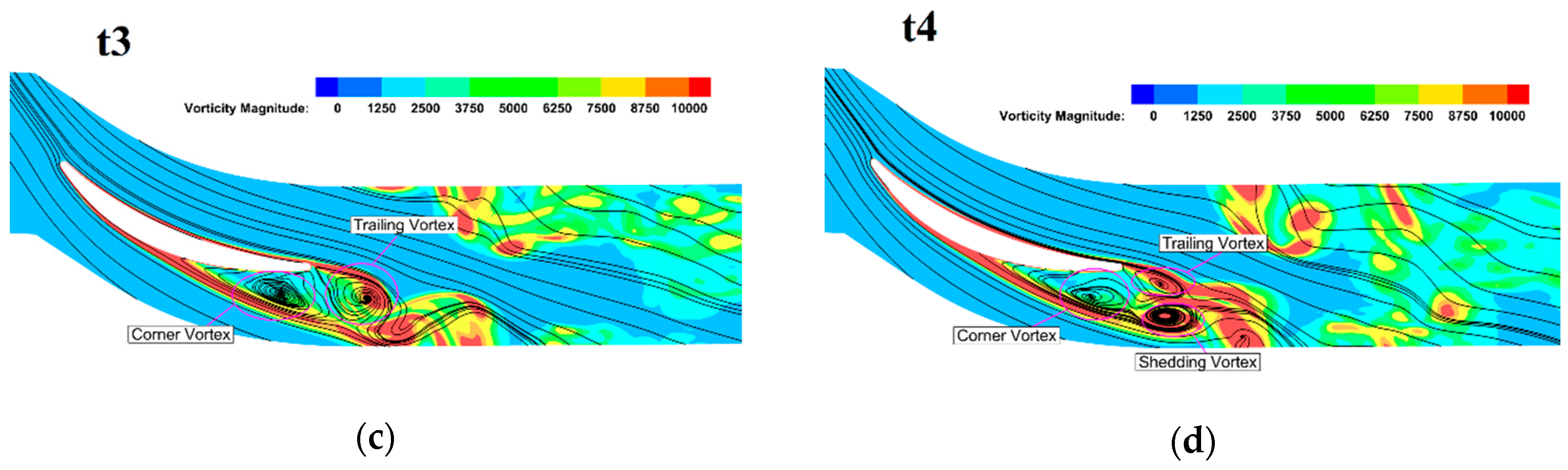
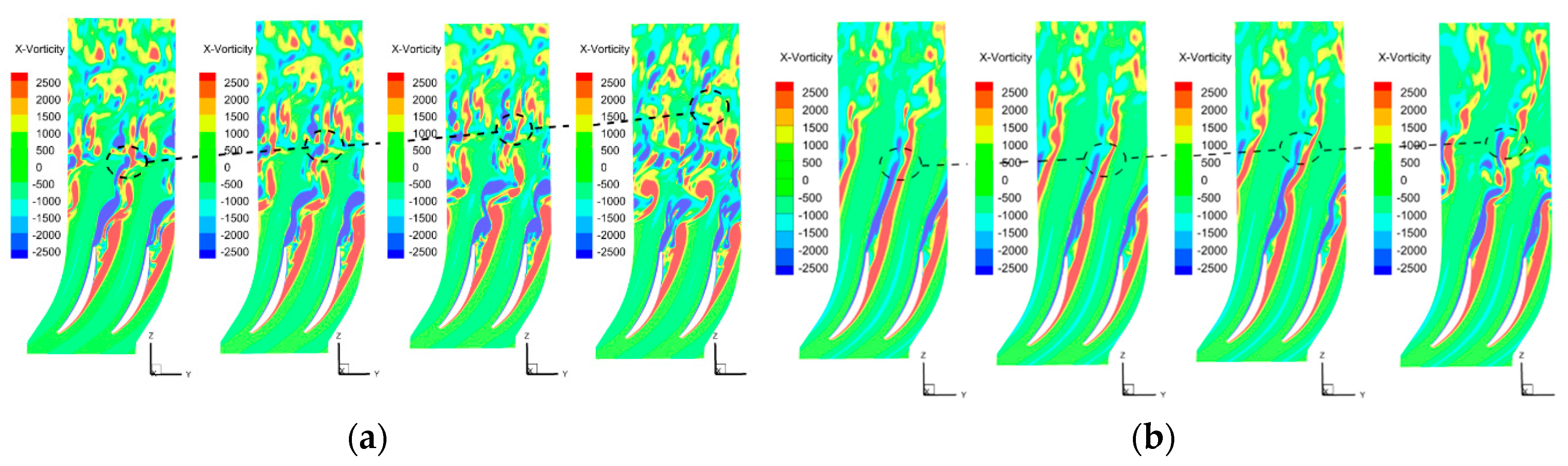
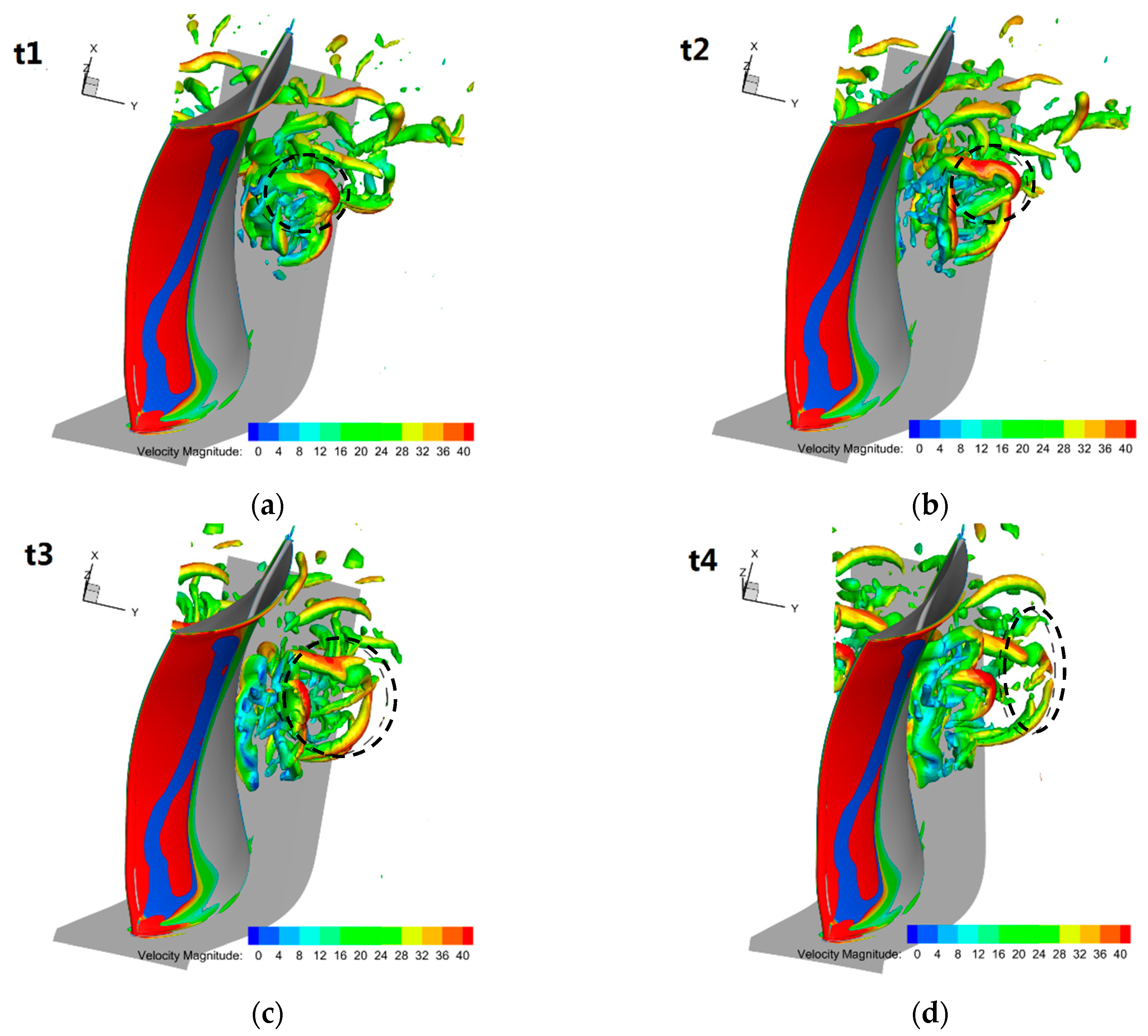
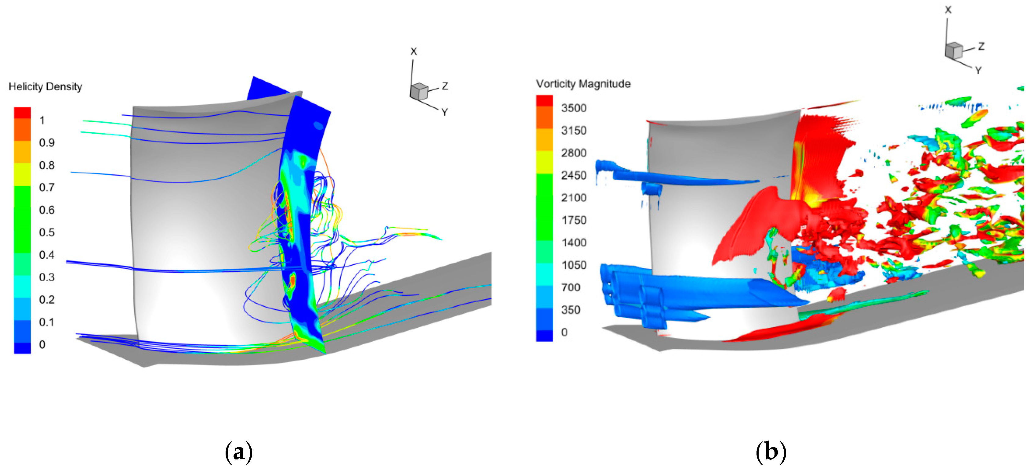
5. Vortical Structures

The unsteady separation structures are illustrated by streamlines at 20% span at different transient cases in Figure 8. Many complex vortices are concentrated in the separation region and downstream, such as the corner vortex (also called separation vortex), wake vortex, and shedding vortex. After the main vortices form in the separation region at t1, the size of the vortices becomes larger and the interaction with each other becomes stronger at t2. Then the corner vortex and wake vortex increase further, but the shedding vortex disappears in the downstream at t3. Another shedding vortex is generated at the following t4.

Figure 9 shows the contour of spanwise vorticity at different transient cases. In general, the separation flow at 20% span is more serious than that at 10% span, which is caused by the introduction of “lean” at the hub of the stator in the process of three-dimensional blade design. The transverse pressure gradient generated by the lean design will drive the low-energy fluids at the hub into the midspan, making the position of the corner vortex move up along the blade, thus altering the behavior of three-dimensional corner region separation. When the corner separation becomes obvious at 20% span, the corner vortex and wake vortex are located in the rear part of the blade. The spanwise vorticity is negative at the pressure surface and positive at the suction surface. The vortices with opposite rotation direction influence each other in the process of moving downstream, showing the strong unsteadiness of the corner separated flows.

In order to better distinguish the vortex structures in the corner separation region, the Q criterion [20] proposed by Hunt et al. is used to identify the turbulence vortex structures at different scales. The definition of Q is as follows:

$$Q=\frac{1}{2}\left({\Omega }_{ij}{\Omega }_{ij}-S_{ij}{S}_{ij}\right)$$

(5)

where Ω_ij and S_ij are the vorticity tensor and shear strain tensor, respectively. Thus, Q represents the local equilibrium of the vorticity tensor and strain rate tensor, as well as the vorticity size.

Figure 10 shows that the vortex structures in the corner are quite complicated. The corner vortex is a combination of multi-scale vortices. The large-scale strip vortices with relatively high velocity exist at the outer edge of the separation region. Meanwhile, the small-scale vortices with relatively low velocity accumulate in the corner region.

Figure 11 shows the development process of strip vortices in the corner separation region. The black dotted region in Figure 11 represents one of the strip vortices. The vortex with a relatively high speed is constantly stretched and bent when it moves downstream. At the same time, many small-scale vortices form and accumulate in the separation region of the suction surface. In the corner separation region, there are many vortex system structures, and it can be inferred that the large-scale vortices with relative high velocity transfer kinetic energy into the small-scale vortices when the stretching process of large-scale vortices is going on, so the turbulence pulsation and energy transform in the corner region are very active.

6. Turbulence Characteristics

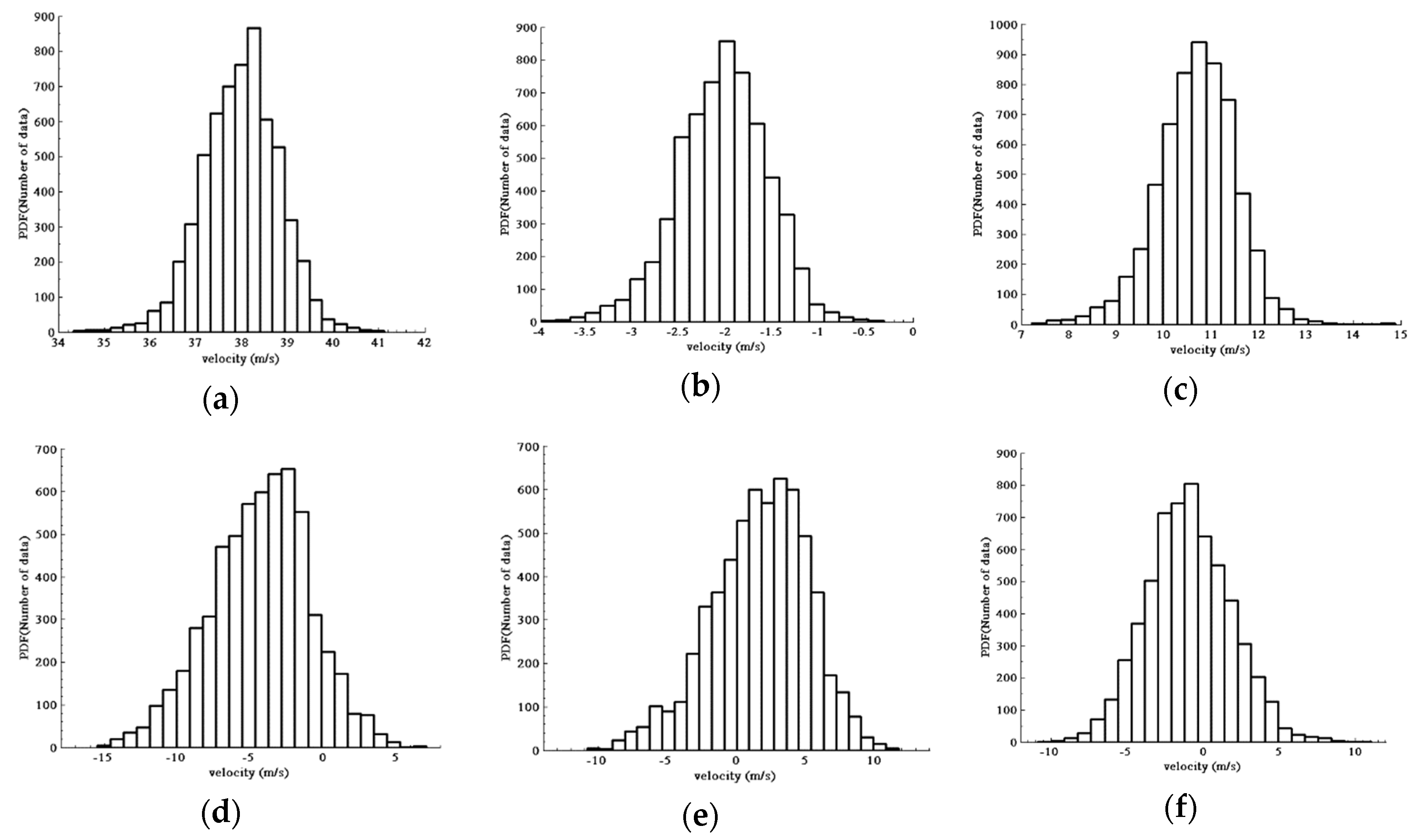
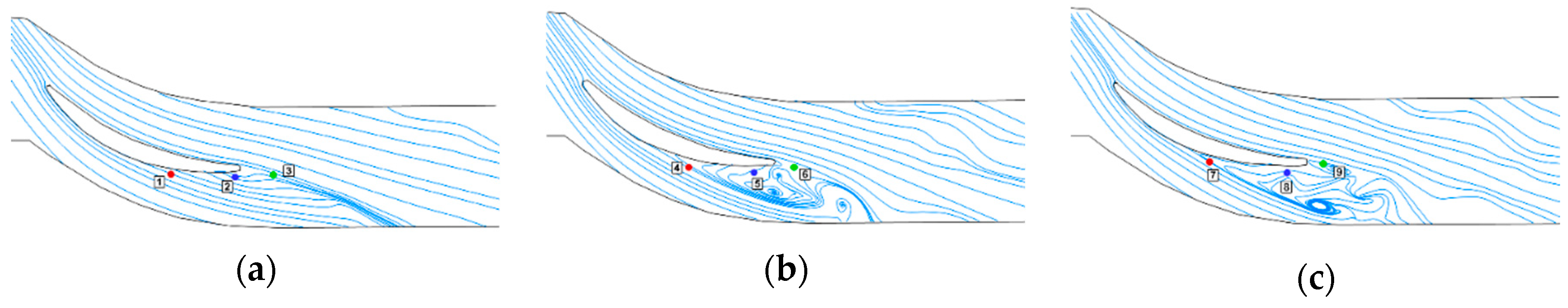
6.1. Statistics Analysis

The unsteady flow structure in the corner separation region is closely related to turbulence behavior. The velocity statistics of two monitor points were analyzed to study the turbulence characteristics of the corner separation flow. Figure 12 shows the locations of two monitor points, which are located in the mainstream region (P1) and the corner separation region (P2). 6000 data samples using velocity probability density function were analyzed. Figure 13 presents the comparison of velocity probability density function (PDF) of monitor points. The PDF of P1 can be fitted into a Gaussian distribution (G1) and the PDF of P2 is a superposition of the two Gaussian distributions (G1 + G2). A similar phenomenon occurs in a low-speed compressor cascade [21]. The velocity probability density of P1 ranges from 36 m/s to 42 m/s, while the velocity probability density of P2 ranges from 1 m/s to 16 m/s. The wider range of P2 indicates the existence of a large number of vortices in the separation region.

Three directions’ velocity data are analyzed by PDF method. Figure 14a–c show that the streamwise velocity PDF of P1 ranges from 34 m/s to 41 m/s, the pitchwise velocity PDF of P1 ranges from 7 m/s to 14 m/s, and the radial velocity PDF of P1 ranges from −4 m/s to −0.5 m/s, so the streamwise velocity plays a major role in three direction velocities. For the monitor point in the corner separation region (P2), the three-direction velocity PDF is basically close, ranging from −15 m/s to 10 m/s, as shown in Figure 14d–f. The reason for the uniform distribution of velocity probability density in the three directions is that the interaction of vortices in the corner region makes the turbulent kinetic energy transport more active.

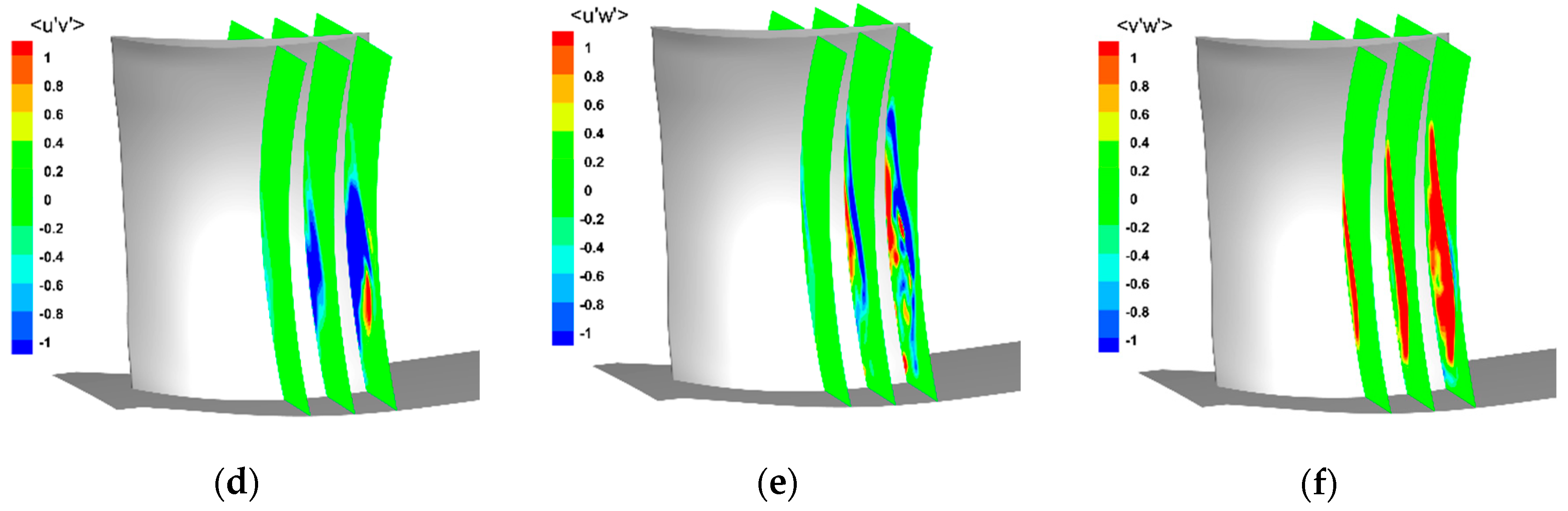
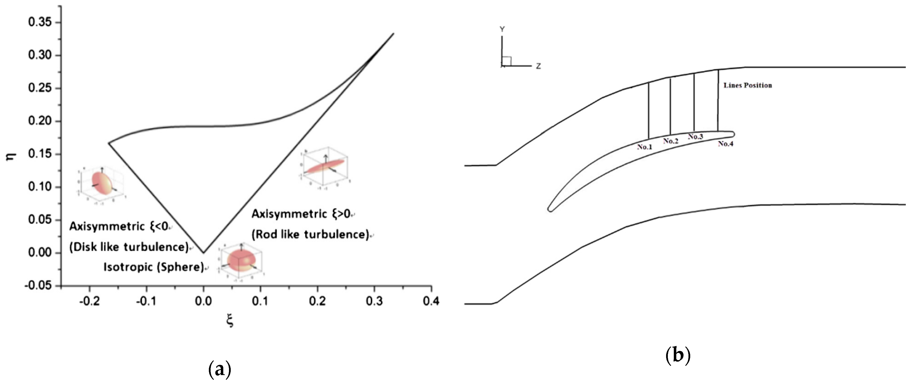
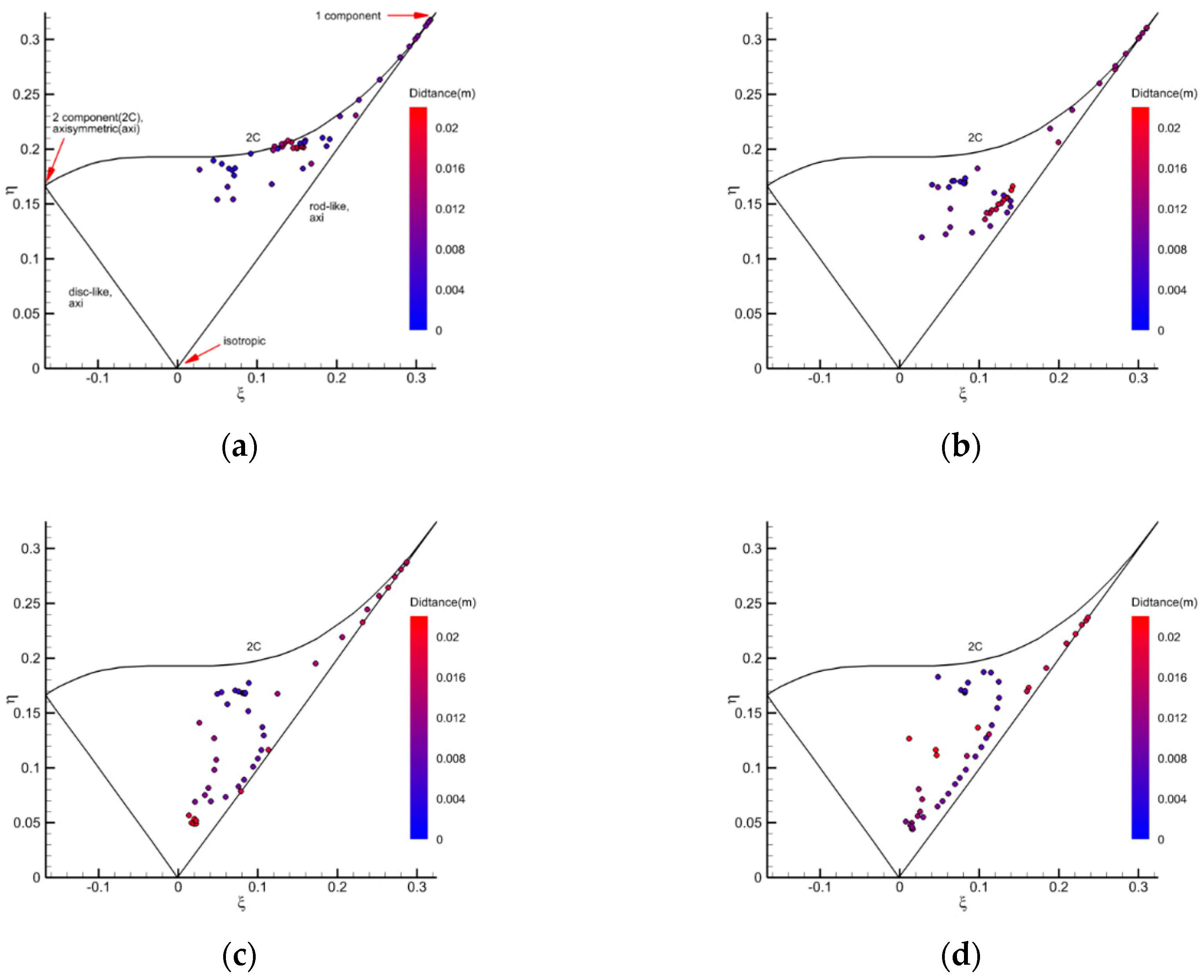
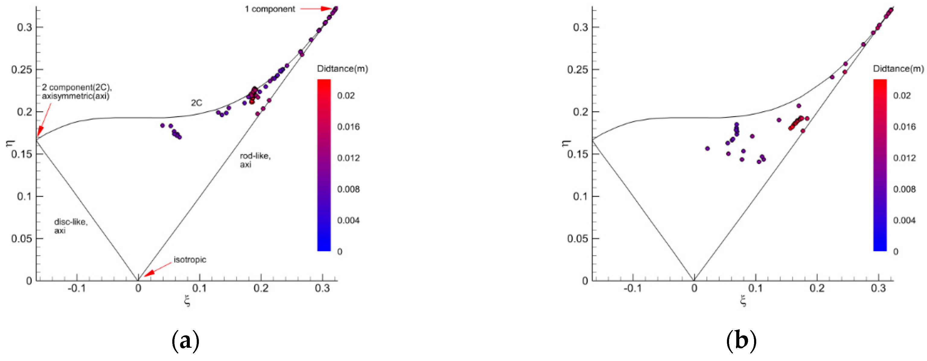
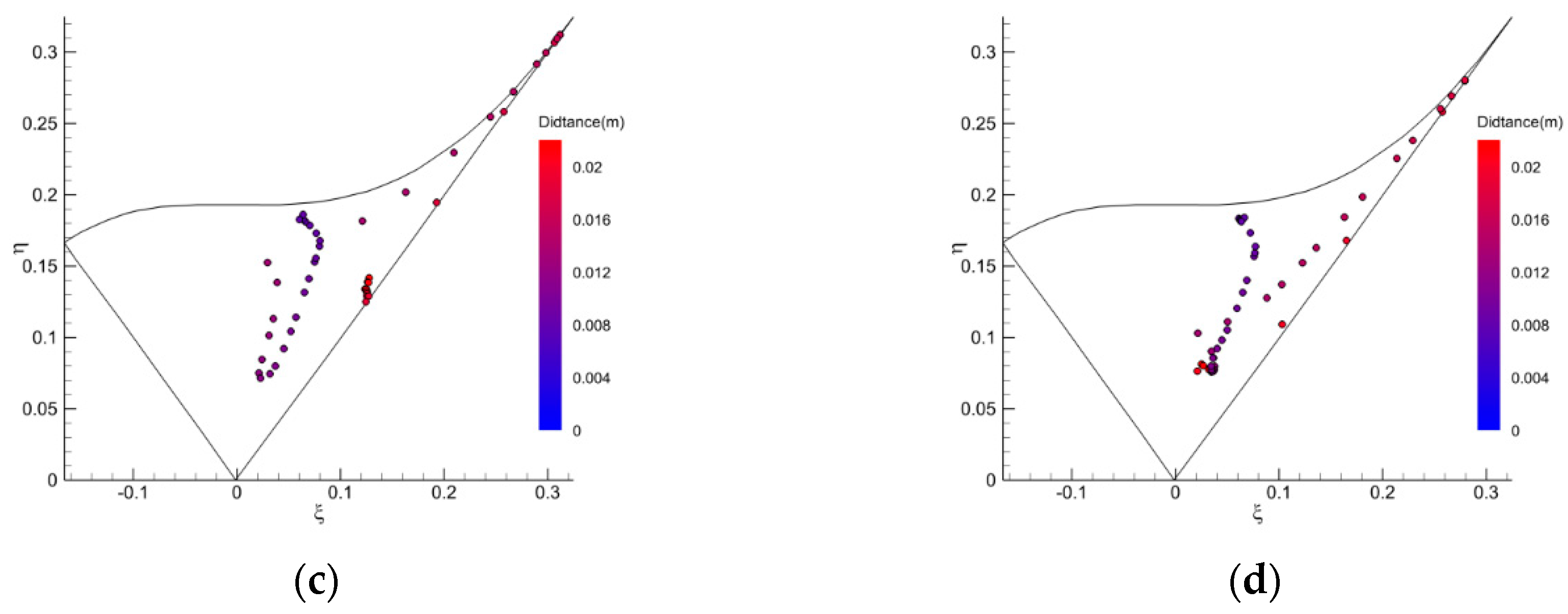
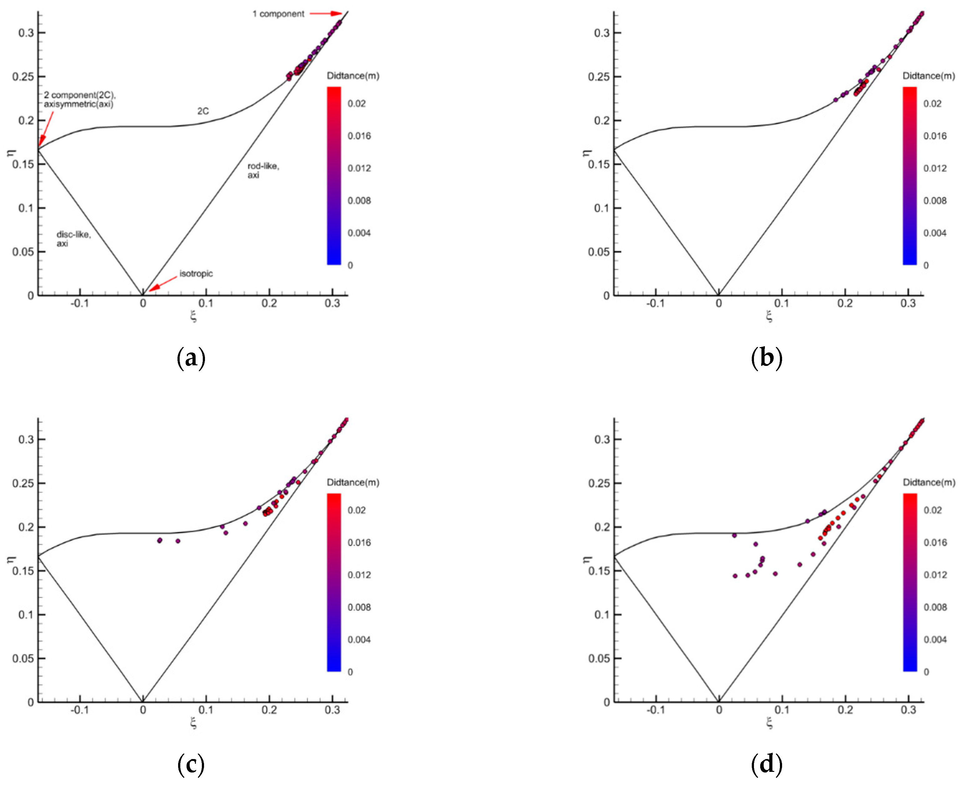
6.2. Turbulence Anisotropy

Figure 15 shows Reynolds stress evolution through the stator passage. The region with large Reynolds stress is located in the corner separation, which reflects the existence of strong turbulence fluctuation. Compared with the spanwise Reynolds normal stress (<u′u′>) and circumferential Reynolds normal stress (<v′v′>), the streamwise Reynolds normal stress (<w′w′>) plays a major role in the flow field. Since the streamwise turbulence fluctuation is greater than the other two directions, the high value region of <u′w′> and <v′w′> in the separation region is larger than that of <u′v′>. The above Reynolds stress analysis reflects the high anisotropy of turbulence.

Lumley triangle theory [22] is used to further characterize the anisotropy of Reynolds stresses in the corner separation region. According to the real physical turbulence, the second and third order invariants of the non-dimension tensor b_ij need to be solved in the triangle theory. The definition of b_ij is as follows:

$$b_{ij}=\frac{{\tau }_{ij}}{{\tau }_{kk}}-\frac{1}{3}{\delta }_{ij}$$

(6)

where τ_ij is Reynolds stress tensor and δ_ij is Kronecker delta. The origin point of the triangle corresponds to the isotropic turbulence, the two solid lines from the origin point represent the axisymmetric turbulence, and the top curve edge of the Lumley triangle represents the two-component turbulence, as shown in Figure 16a. In this paper, in order to explore the distribution of points in the corner separation, several lines used to solve the second-order and third-order invariants were extracted at different spans in the stator shown in Figure 16b. The No.1 to No.4 represent 60%, 70%, 80%, and 90% chord respectively.

Figure 17, Figure 18 and Figure 19 show the distribution of points from the extracted lines in the Lumley triangle at various spans. The colormap represents the y-direction distance from the point to the suction surface of the blade. At 30% span of the blade in Figure 17, the points upstream of the corner separation (No.1) are mainly distributed in the upper right corner of the triangle, indicating that the turbulence state is two-component turbulence. Within the corner separation region (No.2–No.4), the flow state moves toward the rod-like turbulence, suggesting the turbulence to be more anisotropic. The distribution of the points at 20% span in Figure 18 is similar to that at 30% span. As the radial pressure gradient moves the low momentum fluid toward the midspan, the anisotropy of turbulence is slightly weaker. Compared to the 20% and 30% span, the points at 10% span in Figure 19 are mostly concentrated in the upper right corner of the Lumley triangle, which indicates that turbulent state is two-component turbulence or one-dimensional turbulence. Within the wake region, the points near the suction surface move toward the middle of the triangle, suggesting the increase of turbulence anisotropy.

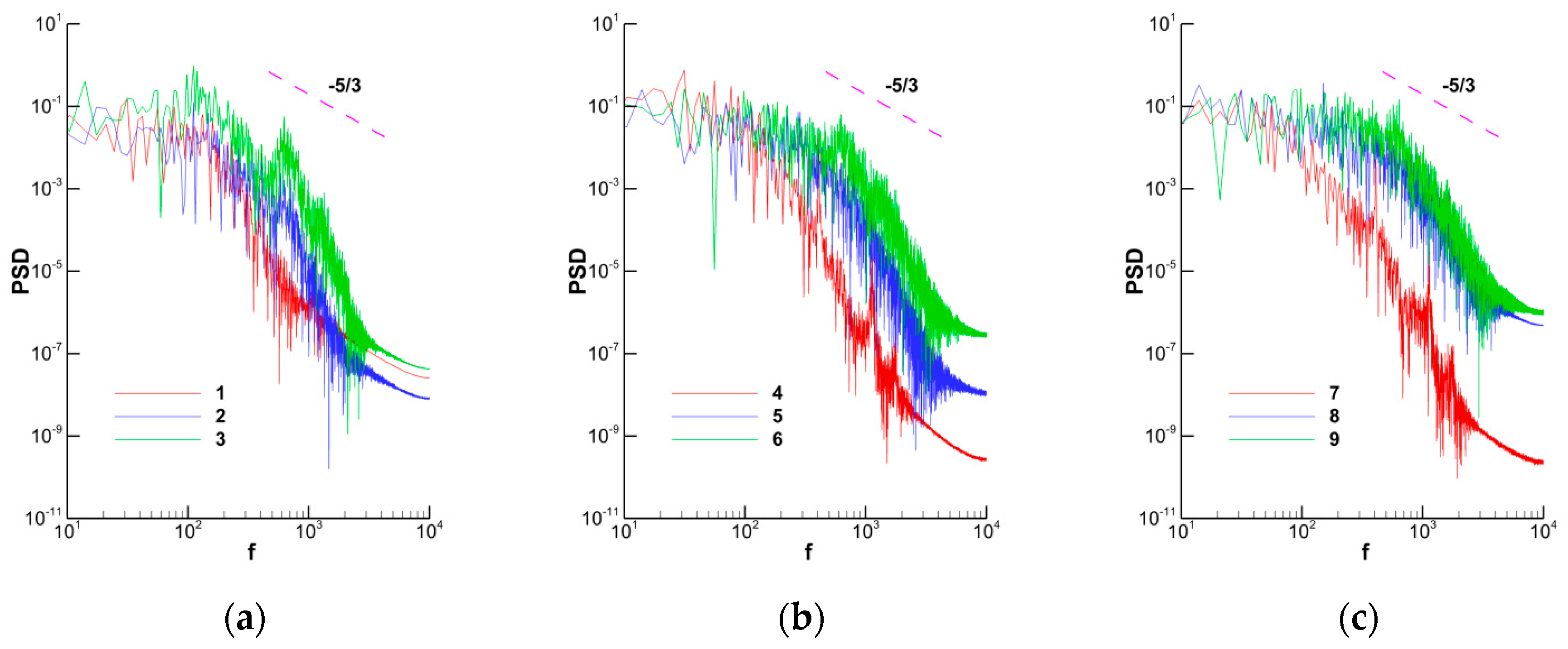
6.3. Turbulence Energy Spectra

In order to study the turbulence energy spectrum of the corner separation flow, monitor points were arranged along the suction surface at different spans, as shown in Figure 20. The fast Fourier transform (FFT) method was used to convert the velocity fluctuation data from these monitor points into the turbulent energy spectra. As can be seen from Figure 21, the energy spectrum of the downstream point was significantly higher than that of the upstream monitor point, indicating that the corner separation region and trailing edge have higher turbulent kinetic energy, and the turbulent kinetic energy concentrates on the large-scale eddies. Compared with the upstream monitoring point, the energy spectra values of the corner separation region and the wake region are of the same order. According to the turbulence theory, when the turbulence is in equilibrium state, the inertial subrange of turbulence follows Kolmogorov’s −5/3 law. It can be seen that the slope of the energy spectra of the monitor point at three spans does not strictly match with −5/3. The −5/3 slope range at 10% span is wider than that of the other two spans, indicating that the turbulent motion there is closer to the equilibrium state. Also, the slope of the points in the corner separation and the wake region at 20% and 30% span is steeper than that at 10% span, indicating that the turbulence is highly unsteady.

Energy backscatter often occurs in corner separation regions with strong shear. Liu et al. [23] showed that there was a correlation between helicity and energy backscatter. When the helicity is greater than 0.6, the energy backscatter is obvious. The helicity h is given by:

$$h=\left|\overrightarrow{u}\cdot \overrightarrow{w}\right|/\left(\left|\overrightarrow{u}\right|\left|\overrightarrow{w}\right|\right)$$

(7)

where $\overrightarrow{u}$ is the velocity vector and $\overrightarrow{w}$ is the vorticity vector. Figure 22a shows the helicity through the stator. The areas with high helicity are mainly concentrated in the corner separation region. Figure 22b shows an isosurface map with helicity density of 0.8 in the stator passage. The color on the isosurface represents the vorticity. The red areas in the figure are mainly located in the corner separation region, indicating that the energy backscatter appears active in these regions, and the development process of the separation flow is always accompanied by the energy backscatter.

7. Discussion

In this paper, the flow structures and unsteady behavior of three-dimensional corner separation in a low-speed compressor stator have been simulated by using the DDES-SA method. The velocity probability density distributions in the mainstream and separation region have been analyzed. The turbulence characteristics in the corner region have been studied, corresponding to the unsteadiness of flow separation. The simulation results have been demonstrated by experiments with good consistency, and the conclusions obtained are as follows:

(1)

Based on the results of the DDES-SA method, the corner vortex, wake vortex, and shedding vortex exist in the corner separation region. A transverse pressure gradient generated by the lean design will drive the low-energy fluids at the hub into the midspan, making the position of the corner vortex move up along the blade. The corner vortex is a combination of multi-scale vortexes. The large-scale strip vortices with relatively high velocity exist at the outer edge of the separation region. At the same time, the small-scale vortices with relatively low velocity accumulate in the corner region.

(2)

The velocity probability density distribution of the monitor points in the corner separation region is approximately the superposition of two Gauss distributions, and the three-direction PDF of the points in the separation region is evenly distributed. The interaction of the vortices in the corner separation region makes the turbulent kinetic energy transport more active.

(3)

High anisotropy of turbulence has been observed in the stator corner separation region. The streamwise Reynolds normal stress plays a major role in the corner region, where the turbulence state develops from two-component turbulence along the top curve edge of the Lumley triangle to “rod-like” turbulence along the right edge of the Lumley triangle, when the turbulence flow moves downstream along the blade suction surface. The turbulent flow in the corner separation region is in nonequilibrium, with the slope of the energy spectra is stepper than −5/3.

References

1. Schulz, H.D.; Gallus, H.E. Experimental Investigations of the Three-Dimensional Flow in an Annular Compressor Cascade. ASME J. Turbomach. 1988, 110, 467–478. [Google Scholar] [CrossRef]
2. Hah, C.; Loellbaeh, J. Development of Hub Corner Stall and its Influence on the Performance of Axial Compressor Blade Rows. ASME J. Turbomach. 1999, 121, 67–77. [Google Scholar] [CrossRef]
3. Weber, A.; Schreiber, H.-A.; Fuchs, R.; Steinert, W. 3-D Transonic Flow in a Compressor Cascade with Shock-Induce Corner Stall. ASME J. Turbomach. 2002, 124, 358–365. [Google Scholar] [CrossRef]
4. Lei, V.M.; Spakovszky, Z.S.; Greitzer, E.M. A criterion for axial compressor hub-corner stall. ASME J. Turbomach. 2008, 130, 031006. [Google Scholar] [CrossRef] [Green Version]
5. Gallimore, S.J.; Bolger, J.J.; Cumpsty, N.A.; Taylor, M.J.; Wright, P.I.; Place, J.M. The Use of Sweep and Dihedral in Multistage Axial Flow Compressor Blading—Part I: University Research and Methods Development. ASME J. Turbomach. 2002, 124, 521–532. [Google Scholar] [CrossRef]
6. Gbadebo, S.A.; Cumpsty, N.A.; Hynes, T.P. Control of three dimensional separations in axial compressors by tailored boundary layer suction. ASME J. Turbomach. 2008, 130, 011004.1–011004.8. [Google Scholar] [CrossRef]
7. Hergt, A.; Dorfner, C.; Steinert, W.; Nicke, E.; Schreiber, H.-A. Advanced Nonaxisymmetric Endwall Contouring for Axial Compressors by Generating an Aerodynamic Separator-Part II: Experimental and Numerical Cascade Investigation. ASME J. Turbomach. 2011, 133, 021027. [Google Scholar] [CrossRef]
8. Spalart, P.R. Philosophies and fallacies in turbulence modeling. Prog. Aerosp. Sci. 2014, 74, 1–15. [Google Scholar] [CrossRef]
9. Spalart, P.R.; Jou, W.H.; Strelets, M.; Allmaras, S.R. Comments on the Feasibility of LES for Wings and on Hybrid RANS/LES Approach. In Proceedings of the AFOSR International Conference on DNS and LES: Advances in DNS/LES, Ruston, LA, USA, 4–8 August 1997; pp. 137–147. [Google Scholar]
10. Wang, Z.; Yuan, X. Unsteady mechanisms of compressor corner separation over a range of incidences based on hybrid LES/RANS. In Proceedings of the ASME Turbo Expo 2013: Turbine Technical Conference and Exposition, San Antonio, TX, USA, 3–7 June 2013; pp. 1–11. [Google Scholar]
11. Xia, G.; Medic, G. Hybrid RANS/LES Simulation of Corner Stall in a Linear Compressor Cascade. Paper No. GT2017-63454. In Proceedings of the ASME Turbo Expo 2017: Turbomachinery Technical Conference and Exposition, Charlotte, NC, USA, 26–30 June 2017. [Google Scholar]
12. Liu, Y.W.; Yan, H.; Lu, L.P.; Li, Q. Investigation of vortical structures and turbulence characteristics in corner separation in a linear compressor cascade using DDES. J. Fluids Eng. 2017, 139, 021107. [Google Scholar] [CrossRef]
13. Taylor, J.; Miller, R. Competing 3D Mechanisms in Compressor Flow. ASME J. Turbomach. 2016, 139, 021009. [Google Scholar] [CrossRef]
14. Zhang, C.K.; Hu, J.; Wang, Z.Q.; Gao, X. Design Work of a Compressor Stage Through High-To-Low Speed Compressor Transformation. ASME J. Eng. Gas Turbines Power 2014, 136, 064501. [Google Scholar] [CrossRef]
15. Zhang, C.K.; Wang, Z.Q.; Yin, C.; Yan, W.; Hu, J. Low-Speed Model Testing Studies for an Exit Stage of High Pressure Compressor. ASME J. Eng. Gas Turbines Power 2014, 136, 112603. [Google Scholar] [CrossRef]
16. Zhang, C.K.; Hu, J.; Wang, Z.Q.; Li, J. Experimental Investigations on 3D Blading Optimization for Low-Speed Model Testing. ASME J. Eng. Gas Turbines Power 2016, 138, 112602. [Google Scholar] [CrossRef]
17. Wang, Z.Q.; Hu, J.; Luo, J.; Li, L.; Gao, X. Investigation of Three-Dimension Flow in a Multi-Stage Compressor Stator. J. Propuls. Technol. 2012, 33, 371–376. (In Chinese) [Google Scholar]
18. Zhang, C.K.; Hu, J.; Li, J.; Wang, Z.Q. Three-Dimensional Compressor Blading Design Improvements in Low-Speed Model Testing. Aerosp. Sci. Technol. 2017, 63, 179–190. [Google Scholar] [CrossRef]
19. Spalart, P.R. Young-Person’s Guide to Detached-Eddy Simulation Grids; Technical Report No. NASA/CR-2001-211032; NASA Langley Research Center: Hampton, VA, USA, 2001.
20. Jeong, J.; Hussain, F. On the identification of a vortex. J. Fluid Mech. 1995, 289, 69–94. [Google Scholar] [CrossRef]
21. Zambonini, G.; Ottavy, X.; Kriegseis, J. Corner Separation Dynamics in a Linear Compressor Cascade. Paper GT2016-56454. In Proceedings of the ASME Turbo Expo 2016: Turbomachinery Technical Conference and Exposition, Seoul, Korea, 13–17 June 2016. [Google Scholar]
22. Simonsen, A.J.; Krogstad, P.A. Turbulent Stress Invariant Analysis: Clarification of Existing Terminology. Phys. Fluids 2005, 17, 088103. [Google Scholar] [CrossRef] [Green Version]
23. Liu, Y.W.; Lu, L.P.; Fang, L.; Gao, F. Modification of Spalart–Allmaras model with consideration of turbulence energy backscatter using velocity helicity. Phys. Lett. A 2011, 375, 2377–2381. [Google Scholar] [CrossRef]
Figure 1. Schematic drawing of compressor test rig.
Energies 13 02123 g001
Figure 2. Stator blade and blade profile: (a) pictorial view of stator blade; (b) profile configurations at three typical blade spans.
Energies 13 02123 g002
Figure 3. Geometric parameters and measuring equipment: (a) stator lean and leading and trailing blade angle; (b) probes and displacement mechanism.
Energies 13 02123 g003
Figure 4. Grid distribution.
Energies 13 02123 g004
Figure 5. The radial distribution of total temperature, flow angle, and velocity at inlet.
Energies 13 02123 g005
Figure 6. Time-averaged static pressure coefficient (Cp) at different spans: (a) 10% span; (b) 30% span; (c) 50% span; (d) 70% span.
Energies 13 02123 g006aEnergies 13 02123 g006b
Figure 7. Loss coefficient (Yp) and exit flow angle (α2): (a) pitchwise mass-averaged loss coefficient; (b) pitchwise mass-averaged exit flow angle.
Energies 13 02123 g007
Figure 8. Streamlines at 20% span at different times: (a) t1; (b) t2; (c) t3; (d) t4.
Energies 13 02123 g008aEnergies 13 02123 g008b
Figure 9. Contour of spanwise vorticity at different times: (a) 20% span from t1 to t4; (b) 10% span from t1 to t4.
Energies 13 02123 g009
Figure 10. Isosurface of Q = 15,000,000.
Energies 13 02123 g010
Figure 11. Isosurface of Q = 30,000,000 at different times: (a) t1; (b) t2; (c) t3; (d) t4.
Energies 13 02123 g011
Figure 12. Monitor point location and contour of velocity magnitude at 20% span.
Energies 13 02123 g012
Figure 13. Velocity distribution of monitor points: (a) P1; (b) P2.
Energies 13 02123 g013
Figure 14. Velocity probability density function (PDF) distribution of monitor points in three directions at 20% span: (a) P1 streamwise; (b) P1 spanwise; (c) P1 pitchwise; (d) P2 streamwise; (e) P2 spanwise; (f) P2 pitchwise.
Energies 13 02123 g014
Figure 15. Reynolds stress throughout the blade passage: (a) <u′u′>; (b) <v′v′>; (c) <w′w′>; (d) <u′v′>; (e) <u′w′>; (f) <v′w′>.
Energies 13 02123 g015aEnergies 13 02123 g015b
Figure 16. Lumley triangle and the position of the extracted line: (a) Lumley triangle; (b) position of lines at 10%, 20%, and 30% span.
Energies 13 02123 g016
Figure 17. Distribution of points from the extracted lines in the Lumley triangle at 30% span: (a) No.1; (b) No.2; (c) No.3; (d) No.4.
Energies 13 02123 g017
Figure 18. Distribution of points from the extracted lines in the Lumley triangle at 20% span: (a) No.1; (b) No.2; (c) No.3; (d) No.4.
Energies 13 02123 g018aEnergies 13 02123 g018b
Figure 19. Distribution of points from the extracted lines in the Lumley triangle at 10% span: (a) No.1; (b) No.2; (c) No.3; (d) No.4.
Energies 13 02123 g019
Figure 20. Location of monitor points at different spans: (a) 10% span; (b) 20% span; (c) 30% span.
Energies 13 02123 g020
Figure 21. Energy spectra at different spans: (a) 10% span; (b) 20% span; (c) 30% span.
Energies 13 02123 g021
Figure 22. Helicity in the corner separation region: (a) contour of helicity density; (b) isosurface of helicity density.
Energies 13 02123 g022