Thermodynamics-Based Process Sustainability Evaluation

Abstract

This article considers the problem of the evaluation of the sustainability of heterogeneous process systems, which can have different areas of focus: from single process operations to complete supply chains. The proposed method defines exergy-based concepts to evaluate the assets, liabilities, and the exergy footprint of the analysed process systems, ensuring that they are suitable for Life Cycle Assessment. The proposed concepts, evaluation framework and cumulative Exergy Composite Curves allow the quantitative assessment of process systems, including alternative solutions. The provided case studies clearly illustrate the applicability of the method and the close quantitative relationship between the exergy profit and the potential sustainability contribution of the proposed solutions. The first case study demonstrates how the method is applied to the separation and reuse of an acetic-acid-containing waste stream. It is shown that the current process is not sustainable and needs substantial external exergy input and deeper analysis. The second case study concerns Municipal Solid Waste treatment and shows the potential value and sustainability benefit that can be achieved by the extraction of useful chemicals and waste-to-energy conversion. The proposed exergy footprint accounting framework clearly demonstrates the potential to be applied to sustainability assessment and process improvement while simultaneously tracking different kinds of resources and impacts.

1. Introduction

The efficient use of energy is of utmost importance for process sustainability and emission reduction [1]. This is an area of increasing research and practical interest that has persisted to this day [2]. All major economic sectors are under investigation, including industry [3], transportation [4] and agriculture [5].

The use of all types of resources and the impacts of processes on the surroundings can be related to the use of the energy necessary to complete the tasks. The evaluation of industrial systems is most frequently performed by using mathematical models for the consistent estimation of their thermodynamic properties and related energy use. Commercial simulators provide this functionality [6].

When comparing alternative processes, the energy demand is not always a suitable metric because it may not take into account the quality of the energy used. In this context, exergy is the property that can be used as a combined indicator of energy quality and quantity [7]. This property of exergy allows the optimisation of the process design and operation based on realistic estimates of how much energy can be sourced, converted, supplied or reused. Extended Exergy Analysis also takes into account the economic aspects of a resource; e.g., a wind turbine in a more windy place has a higher exergy efficiency because it produces more energy with similar investment and operation costs [8]. This concept can be applied to an isolated unit (e.g., a wind turbine), to an industrial process (e.g., concrete industry [9]) or a farming system (e.g., canola [10]).

Process systems can no longer be considered in isolation [11], dealing only with the maximisation of their standalone efficiency. While process efficiency is important for obtaining profit, its environmental impact spans beyond the boundaries of the current system. This conflict between the usefulness of the streams and resources of a process and their effect on natural storage is solved by the concept of circularity [12], in which the overall life cycle is considered.

The exergy concept has been shown to be key to addressing sustainability issues [13]. The use of renewable resources is beneficial, as this takes advantage of natural energy flows across the Earth, without depleting accumulated terrestrial energy reserves, such as fossil fuels [14]. Therefore, the share of renewable resources used in the economy should be increased, although the exergy obtained in some of the harvesting paths may be small. Another confirmation of the usefulness of exergy for sustainability modelling comes from the domain of water management and water treatment plants [15]. However, despite being proven to be potentially useful, the use of the exergy concept is frequently limited only to the estimation of the exergy efficiency of various process contexts [16], such as the exergy efficiency of a process or the share of exergy from the renewables provided to a process.

There are examples of exergy assessment in the literature. Changes in the concentration of a solvent give rise to a massive exergy loss, indicating the importance of solvent selection [17]. An exergy analysis to evaluate the performance of a continuous Directional Solvent Extraction (DSE) desalination process using octanoic acid was presented in [18]. Extractive solvent regeneration is a potential method to substitute stripping and reduce the exergy demands of CO₂ capture systems [19].

To compare process alternatives using exergy, the selection of system boundaries and reference points (e.g., ambient conditions) must provide comparable output streams. The same issue is also typical for the implementations of the Life Cycle Assessment (LCA) framework [20], where the choice of the system boundary and selection of life cycle stages is crucial to obtaining credible results. This similarity is useful for the potential integration of exergy-based criteria within the framework.

There have been many attempts to define a universal reference state [21]. The restricted dead state is defined as the physical thermodynamic equilibrium with the reference state. However, a dead state which takes the chemical equilibrium into account is required for environmental assessments. A widely used variant is based on an Earth similarity condition [22], where a reference substance is chosen for every element [23]. Substance exergies are determined to start from those of the reference substances, considering balanced chemical reactions. Regretfully, some chemical exergies are negative, and the reference is not entirely consistent [24].

The initial reference state has been updated according to new and more accurate geochemical and geological information. Thanatia [25] is a thermodynamically dead planet in which all materials have reacted, dispersed and mixed; i.e., it represents a complete dispersed state of minerals and the complete combustion of fossil fuels. Thanatia is not a reference state but a baseline used to calculate concentration exergies, therefore providing the exergy replacement costs. To assess the exergy degradation of the natural capital, the reference environment has evolved to a Thermo-Ecological Cost (TEC) methodology which in combination with the concept of Exergy Replacement Costs (ERC) results in the TERC (Termal-Exergy Replacement Cost) methodology, which is used to assess the degradation of fossil and mineral capital [25].

The choice of the reference conditions can also have a significant effect on the evaluation of the chemical exergy of particular substances such as fuels [26]. This is even more important for the evaluation of the exergy efficiency of large-scale systems, such as the Turkish industrial sector. A study of the trends in this area [27] revealed an increase from 25% to 29% when the ambient reference temperature decreased from 298 to 273 K.

From the perspectives of ecological modelling and the life cycle, it is possible to use the concept of embodied exergy: the cumulative amount of exergy inputs necessary to deliver a product or a service [28]. The cited work has applied the concept to exergy costing and accounting for energy sector applications, linking exergy spending to monetary costs.

Although exergy is very useful for assessing the loss of resource quality, its use has not been widespread in environmental impact evaluation. LCA is one of the well-established techniques with which exergy has been combined to conduct the exergy analysis of a complete product life cycle [29].

One method to quantify the environmental impact of a process based on exergy is the use of the environmental compatibility indicator, which takes into account the input exergy to the process and the exergy requirements for the abatement of process emissions and waste [30]. In an ideal case (no impact considered), the discussed process emits only heat.

Furthermore, the highest exergy efficiency does not correspond to minimum costs [31] or minimum environmental impact [32]. Exergy efficiency, in that sense, is a local evaluation criterion and is only appropriate to specific energy conversion or use schemes.

Circular economic flow is based on the separation of technology and the economy as the main condition [33]. This concept considers the inputs and outputs of operations during industrial production and focuses on cause-effect relationships. The author considers the circularity concept in terms of temporally repeating cycles of economic activity and presents the realisation that the economy cannot be considered separately from the environment.

Different industrial approaches to the improvement of the sustainability of human society and the environment have been attempted. The simple approaches to the substitution of materials and the end-of-pipe reduction of harmful emissions have been superseded by LCA-based methods for ecological design and economics [34]. The understanding of the interconnections, inputs and outputs for the entire supply leads to the goals of the circular economy [35]. In this context, close attention has to be paid to the full life cycle, including the facility construction and decommissioning, as has been shown in an analysis of the reuse of materials from wind turbines after their end of service [36].

The utilisation and reuse of different types of waste may be analysed by systematic approaches: e.g., P-Graph offers a solution for closed-loop processing and the analysis of its impact [37]. Process Integration also has great potential for analysing circular flows, especially in improving the sustainability of energy systems [38].

For the effective application of targeting and optimisation models in the design, operation and retrofitting of industrial processes for the circular economy, it is necessary to have flexible and scalable modelling concepts and tools. Conventional logic treats process streams as either inputs or outputs, where the outputs are either products or waste streams [39]. The waste streams were traditionally thought of as needing to be treated and disposed of. The circular economy paradigm for process design [40] requires non-product outlet streams to be treated as sources of potential resources as well.

Besides research, regulatory action has also been taken; for example, the EU action plan for the circular economy [41]. Some ideas related to circularity have been developed previous to the popularisation of the circularity concept; e.g., reuse, remanufacturing or recycling [42]. Sustainable Consumption and Production (SCP) tools have been identified as a booster of circularity [43]. The implementation of circularity has resulted in innovation opportunities [44]. This is the case with the redesign of pharmaceutical supply chains to prevent the waste of medical supplies [45].

A clear example of circularity is the mass flow in nature [46]: a mixture of dead biomass is decomposed by microorganisms and fungi to simple molecules that are captured by plant roots to generate complex molecules again using solar energy. This nutrient flow takes place in natural environments but not in agriculture, where the products are transported away to consumers without returning back to fields [46], breaking the natural cycle.

There is intensive research available in the literature about circularity in the industry, such as in metals processing [47], including copper [48] and steel [49]. Other fields have also been researched, such as construction [50] or forest wood harvesting and utilisation [51]. However, the global economy is not circular because large amounts of materials are used only once to provide energy or commercial value and are thus not available for recycling [52].

Examples of circularity in the chemical industry are related to plastics recycling as a consequence of the strategy of the European Commission [53]. The practices include plastic sorting [54], product design [55], or the design of chemical bonds suitable for biodegradation [56].

Many authors have defined circularity and its advantages and provided tools to quantify it. Examples include Corona et al. in 2019 [57], who focused on the circularity metrics, and Sassanelli et al. [58], who dealt with the assessment methods and the identification of the systematic taxonomy of the indicators used for circular economy evaluation by Saidani et al. [59].

The provided state-of-the-art review has shown that various tools and practices are available for process network optimisation, allowing the identification of the potential reuse paths for material components. However, accounting for the reuse of multiple resources within complex networks, containing multiple loops, creates a multi-dimensional optimisation problem if only approached directly. This observation reveals the need for an accounting framework and concepts that would measure the degree of sustainability and favorability of process networks adequately, taking into consideration the heterogeneous nature of the networks both in terms of their activities and the multitude of resources tracked.

The current work presents a system of analytical concepts, a framework and tools for evaluating the impacts of process systems based on thermodynamics. The framework is based on the concept of exergy as the unifying performance metric. It defines the tools of exergy assets and liabilities that enable the assessment of the sustainability of the considered systems. The trade-offs between the different feedstock and product flows and environmental impacts are modelled using the exergy assets and liabilities, leading to the calculation of the exergy footprint. The remaining content of the article presents the model and framework (Section 2), followed by illustrative case studies (Section 3) and a concluding discussion in Section 4.

2. Model and Framework

Process systems and supply chains consist of various process units and sub-systems, each of them having input and output interfaces and internal relationships. The heterogeneity of processes and their characteristics are complemented by the system scalability: the ability of various process units and systems to be integrated as parts of larger systems, forming nested hierarchies. This section starts with the development of the modelling concepts and framework, including the material flow cycles and the energy cascading principle; that is followed by the formulation of the accounting framework and the modelling equations.

2.1. General Trends and Issues

To derive a unifying criterion for the assessment of heterogeneous process systems of varying sizes, it is necessary to formulate a suitable framework. This should be based on a common process representation and allow the scalability of the evaluation scope. An essential property of the desired framework is that it be based on indicators that quantify the resource supply, demand, availability and deficit in a seamless way. The quantitative criteria also have to reflect the need to attain a sustainable development path of the considered system. These requirements form the basis for selecting reference conditions for the desired system designs.

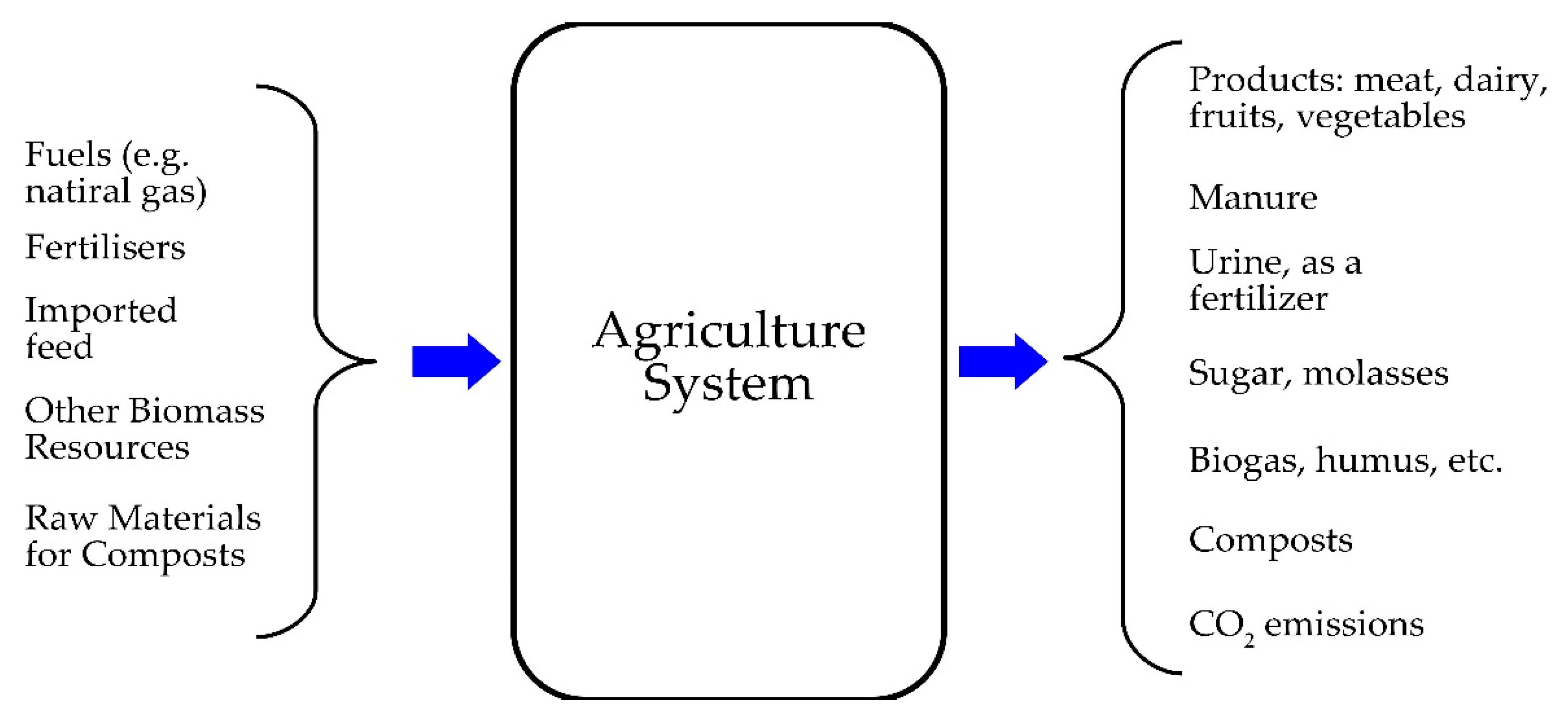
At the process level, there can be multiple inputs and outputs. An example can be taken from the domain of agriculture [60]. As illustrated in Figure 1, there are various input streams as well as output streams, which are of different natures and have different environmental impacts and economic significance. While input-output analysis is helpful in quantifying the net resource and footprint impacts, it is difficult to use in revealing possible reuse and recycling patterns because of the different natures and compositions of the inlet and outlet streams.

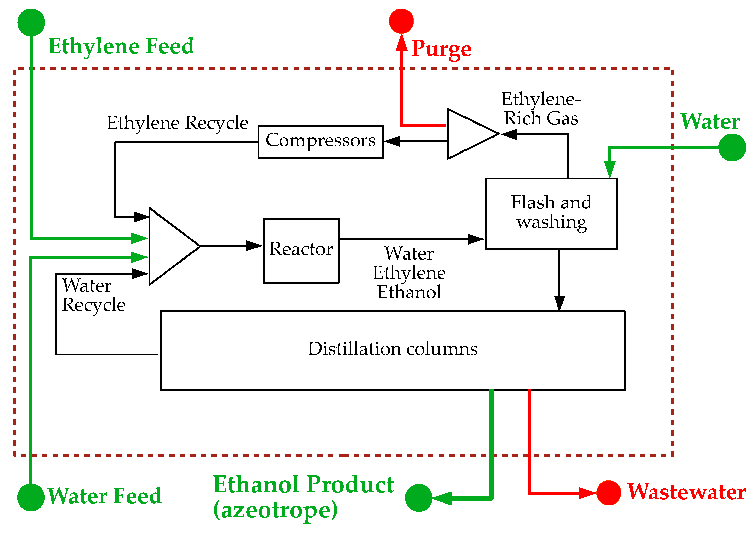
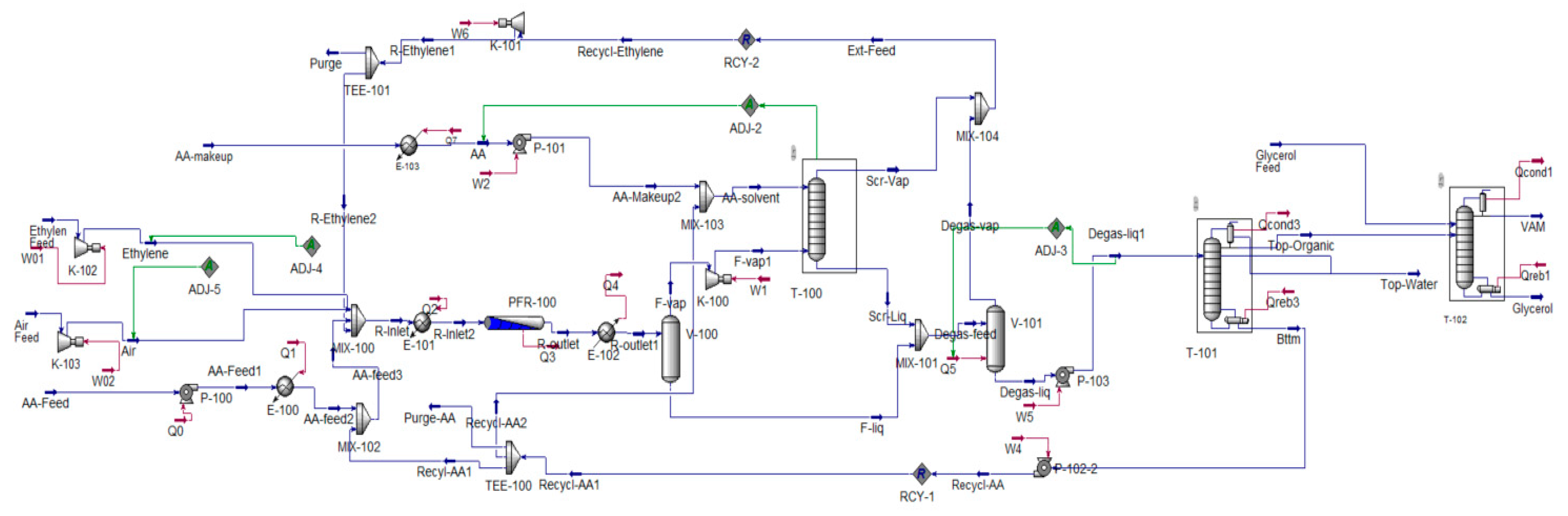
They are good examples of recycling from chemical processes involving reactors at the process level, where the unreacted feed is separated from the reaction products and recycled. Such an arrangement can be found in the ethanol production process by the hydration of ethylene [57]. The usual pattern is a reactor (or a reactor network) followed by separators. Figure 2 shows a summary of the process arrangement of the example given in [61]. The key reactants are ethylene and water. First, the ethylene is separated by flashing and washing, and then the resulting water–ethanol mixture is separated in a series of distillation columns. The system features two loops: one for the ethylene recycling and another for the water recycling.

Several types of nexuses have been discussed in the research literature. Of these, the best-known is the energy–water nexus [62], but the correlations among other resources and product flows have also been investigated; for example the energy–water–food nexus [63], the joint consideration of water, land and food [64], and even the consideration of terrain–emission interactions [65]. All these nexuses can be represented as having two major parts: material and energy flows. An analysis of these two parts is presented below.

2.1.1. Material Flows and Their Cycles

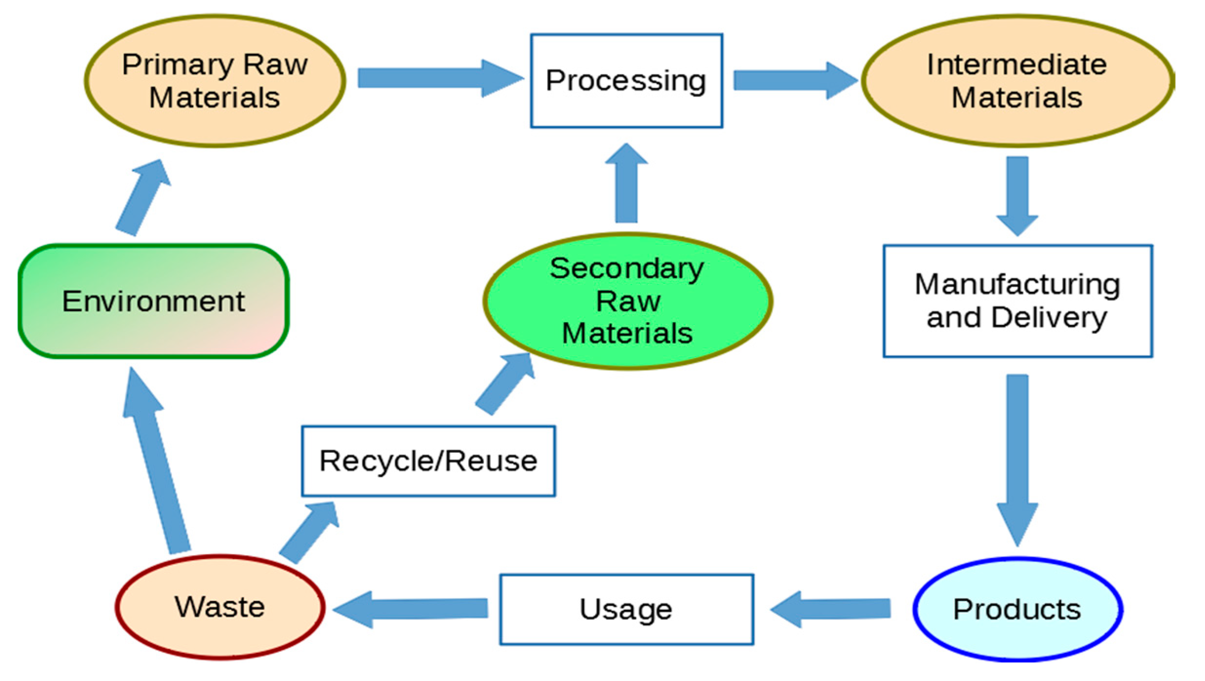
At the regional level, placing industrial sites within the environmental context reveals that the significant material flows feature two types of cycles (Figure 3), which can be extrapolated to a global (planetary) level. One type of material cycle is the traditional one: extracting resources (primary raw materials) from environmental storage sites, processing them into intermediate materials and further to products, the delivery and use of those products, the generation of waste streams and the disposal of the waste into the environment. The second cycle travels a shorter path, consisting of diverting part of the material flow of waste to the generation of secondary raw materials, which are used to substitute primary raw materials. Of these cycle types, the traditional route is more straightforward and is perceived as economically more favourable. While this may have been the case at the beginning of the industrial age, the increasing waste generation makes the recycling–reuse pattern desirable and viable for key materials such as paper [66], metals [67], and even electronic waste [68].

One obvious essential feature is that both material flow patterns form closed cycles. In this sense, the major degree of freedom within the material flows network is the split between the recycled and non-recycled fractions of the generated waste.

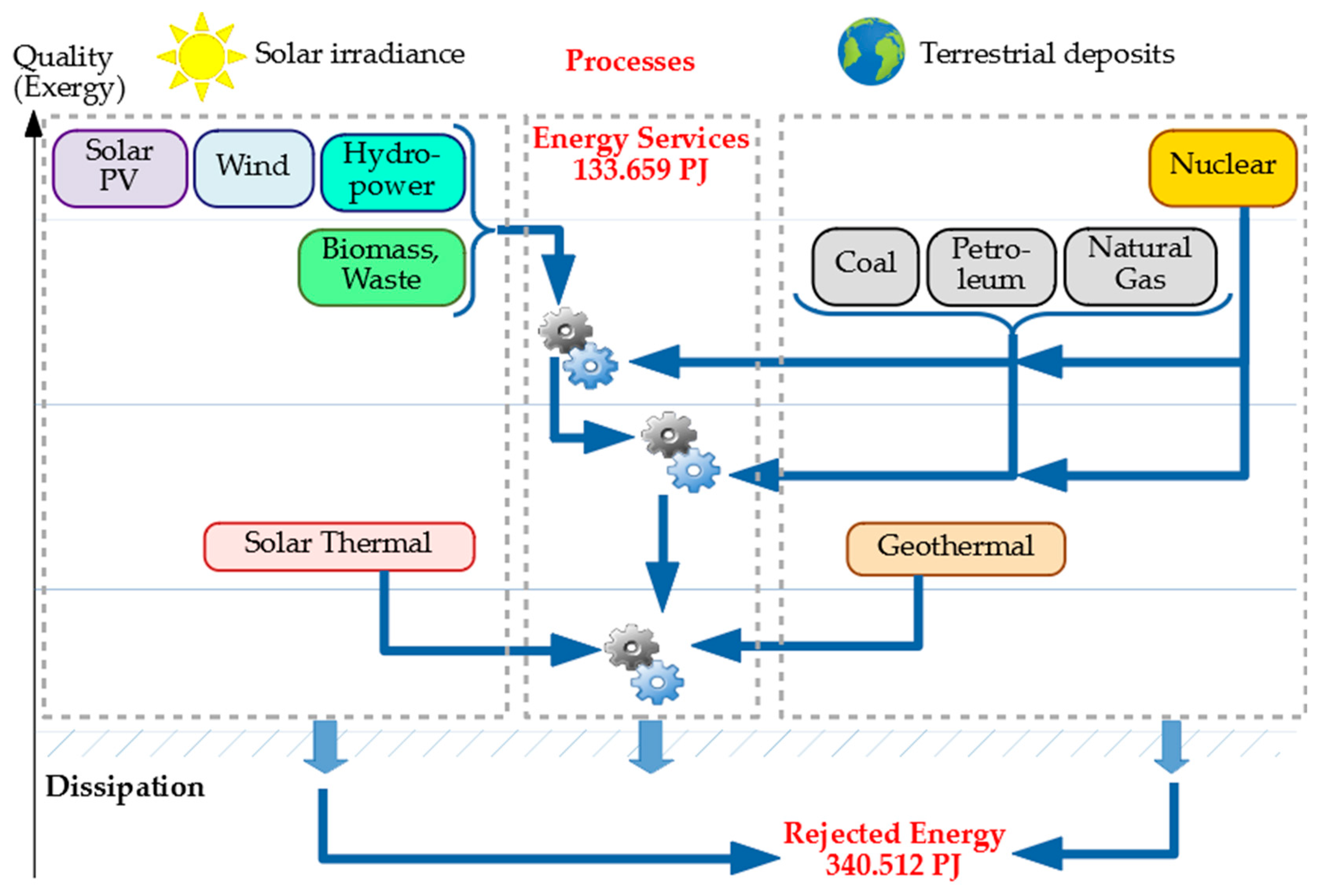
2.1.2. Energy Flows—Cascading

Energy can be sourced either from renewable sources (mainly of solar origin) or from terrestrial deposits (Figure 4). Energy flows follow the Laws of Thermodynamics, cascading from higher to lower quality [69]. Harvested energy flows can be used to power various processes, resulting in the movement of the material flows within a system; i.e., an enterprise, a municipality, or a region. At the system level, at various scales, energy can be sourced, converted and used and ultimately is left to dissipate in the environment. The share of the losses to dissipation reaches two-thirds [70]. This pattern reveals that there are two types of global system interface flows: energy inlets (renewable) and energy outlets (dissipation). Any non-renewable energy sources are internal to the system. This allows the classification of renewable energy sources as long-term degrees of freedom and the non-renewable as short term ones.

Energy cascading is thus used to power the closed material cycles for industrial and other activities in the global economy. Establishing this principle allows us to set up a framework for system state accounting which can be used to evaluate and optimise the system design and operation for various objective functions linked to the energy supply.

The analysis in this section clearly points to energy harvesting and use as the dominating factor, representing a key degree of freedom in driving the economy and societal activities. Moreover, energy is stored in various forms for conversion, transport and use. This view of energy transformations allows the consideration of industrial and business processes as networks of states and transitions, where the states are related to the energy content of materials and process streams, while the transitions are either intentional process operations or spontaneous transitions, transforming process streams from one state to another at the expense of exergy conversion and destruction.

There have been many proposed circular economy indicators; e.g., a recent review [59] analysed 55 sets of circularity indicators. The choice and most beneficial use of indicators depends on the considered context. Within the context of a given supply chain or an industrial process, the degree of recycling of key materials is the most widely used indicator; in this context, the Circular Material Use rate (CMU) has been adopted by Eurostat [71] to determine the degree of circularity of systems at various scales. In the case of Eurostat, this is applied to measure the circularity of the economies of EU member states. CMU is defined, within the context of a specific material, as the fraction of the recycled material (U) within the overall material intake by the system (M):

$$\mathrm{C}\mathrm{M}\mathrm{U}=\frac{\mathrm{U}}{\mathrm{M}}$$

(1)

While CMU is a crucial indicator, it alone is not sufficient to characterise the sustainability of the considered systems. Additional indicators are therefore needed to provide sufficient characterisation. The model proposed here uses energy as the main indicator, in the form of exergy, with all remaining system properties used as specifications to ensure the sustainable conditions of all parts of the environment–economy–society macro-system.

2.1.3. Exergy as the Unifying Performance Metric

The identified need for an energy-based indicator needs to be put in the correct context. The process systems are evaluated based on certain requirements, which are intended to minimise or eliminate any adverse environmental impacts of the system.

Referring to Figure 3 and Figure 4, the material outputs of each process system cannot simply be released to the ambient environment. Before release, they have to be brought to a certain desired state at the point of release to the environment characterised by composition (or an equivalent specification) and temperature. Naturally, suitable pressure also has to be selected and specified.

Such a state is usually defined by the environmental regulations concerning the corresponding natural storages. For instance, for wastewater discharge to environmental basins in the European Union, it is required that they contain a maximum of 25 mg/L BOD5 (Biological Oxygen Demand) at 20 °C [72], which can be used to estimate the content of the main contaminants.

Similarly, there are regulatory limits on effluent discharge temperature. For instance, King County, Seattle, US [73], allows a maximum of 40 °C at the entry of wastewater treatment plants. The Environmental Protection Agency of Taiwan [74] imposes limits from 35 to 42 °C for the points of discharge at sea, with the addition of a requirement that the water stream does not deviate from the surrounding surface water by more than 4 °C. The significance of this stipulation is that it relates the target stream temperature to that of the ambient conditions.

From the above reasoning, it becomes clear that all energy flows and storage contents that relate to the considered process systems are limited only to the energy that can be extracted as a difference from the conditions of the surrounding environment. This is equivalent to the definition of exergy, also known as availability [69].

In this case, the referenced environmental conditions are not necessarily the currently existing conditions but those mandated in the environmental regulations and standards. This provides a reference point for estimating the exergy balance (deficit or excess) to achieve zero deviation from the desired environmental conditions and minimise the potential environmental impacts.

The observations below aid in establishing the basis of the evaluation model:

(1)

For any process system, only the interface streams—inputs and outputs—can be considered as producing environmental impacts. Internal streams have no direct impact on the environment.

(2)

The inputs represent the demands of the system which are passed to upstream providers of resources, products and services. Similarly, the outputs represent the interface with their downstream counterparts: users/consumers, utilities, artificial (landfills, tailing ponds) and natural storage systems (the atmosphere, rivers, lakes, oceans, the ground).

The next section defines the necessary elements for using exergy as the metric to determine the quality of a process stream by defining exergy components associated with the stream, divided into assets and liabilities. The follow-up sections build on this by formulating the overall framework for exergy accounting and computing the exergy profit or loss associated with a process system.

2.2. Exergy Accounting Framework

For the evaluation of a process system’s performance regarding its environmental impacts and its sustainability, it is necessary to capture the interfaces—i.e., the inlet and outlet streams (Figure 2)—as only they have the potential for impact. The internal constraints and internal flows are resolved by the system calculation model; i.e., simulation or optimisation. EXA and EXL denote the exergy assets and the exergy liabilities of a stream, respectively.

Consider again Figure 2, in which the input and output streams are highlighted. The process inputs are the streams labelled as ethylene feed, water feed, and water (wash water). The outputs are the streams labelled as “purge”, wastewater, and ethanol product.

Inputs and outputs can be distinguished from the interface streams. An output stream is either a product or waste. In the case of product output, liabilities are not assigned because a product stream only carries useful value but does not involve the exergy penalty. Exergy assets can be assigned to a product stream only if the stream content implies or has the goal of retrieving exergy capable of driving economic activities such as chemical processes or transport operations.

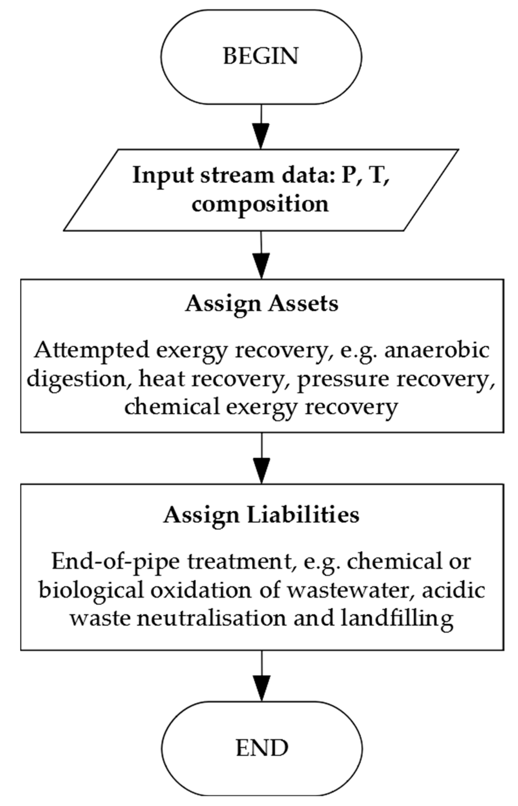
For waste streams, the determination of exergy assets or liabilities employs a notional (potential) workflow (Figure 5). The workflow involves attempted operations for exergy extraction/recovery first, followed by the end of pipe treatment of the residual stream and finally discharge. Any potential for exergy extraction and utilisation is defined as an asset, and the need to add exergy to the remaining potential workflow is added to the liabilities.

The input streams to the processing system have to be considered. For this, it is necessary to realise that the input to any human-operated process system is a product output of an upstream system. This includes, besides intermediate products, the resource streams extracted from nature (since the extraction itself is already an operation). Following the principles defined for products, the direct exergy liabilities are not assigned to the input streams, while exergy assets are assigned only in the case of an energy conversion system as the main object of evaluation.

The above discussion only reflects the perspective of the local to downstream impacts of a process system. To enable accounting for complete supply chains as well as the overall LCA [75], it is important also to include the upstream environmental impacts, leading to the need to account for the embodied exergy [28]. In this case, instead of the potential downstream exergy flows, the account includes the upstream exergy inputs (liabilities/credit) and the exergy content of the evaluated streams, assigned as assets.

Having estimated the exergy assets and liabilities for each of the interface streams for a process system, they are summed up, producing the total exergy assets (Equation (2)) and the total exergy liabilities (Equation (3)) of the system.

$$\mathrm{E}{\mathrm{X}}_{\mathrm{a}\mathrm{s}\mathrm{s}\mathrm{e}\mathrm{t}}={\displaystyle \sum }_{\mathrm{i}\mathrm{n}\mathrm{p}\mathrm{u}\mathrm{t},i}\mathrm{E}{\mathrm{X}}_{\mathrm{a}\mathrm{s}\mathrm{s}\mathrm{e}\mathrm{t},i}+{\displaystyle \sum }_{\mathrm{o}\mathrm{u}\mathrm{t}\mathrm{p}\mathrm{u}\mathrm{t},j}\mathrm{E}{\mathrm{X}}_{\mathrm{a}\mathrm{s}\mathrm{s}\mathrm{e}\mathrm{t},j}$$

(2)

$$\mathrm{E}{\mathrm{X}}_{\mathrm{l}\mathrm{i}\mathrm{a}\mathrm{b}\mathrm{i}\mathrm{l}\mathrm{i}\mathrm{t}\mathrm{y}}={\displaystyle \sum }_{\mathrm{i}\mathrm{n}\mathrm{p}\mathrm{u}\mathrm{t},i}\mathrm{E}{\mathrm{X}}_{\mathrm{l}\mathrm{i}\mathrm{a}\mathrm{b}\mathrm{i}\mathrm{l}\mathrm{i}\mathrm{t}\mathrm{y},i}+{\displaystyle \sum }_{\mathrm{o}\mathrm{u}\mathrm{t}\mathrm{p}\mathrm{u}\mathrm{t},j}\mathrm{E}{\mathrm{X}}_{\mathrm{l}\mathrm{i}\mathrm{a}\mathrm{b}\mathrm{i}\mathrm{l}\mathrm{i}\mathrm{t}\mathrm{y},j}$$

(3)

Equations (2) and (3) can be applied to various contours, including specific process systems, supply chains or complete life cycles. They can be used to evaluate downstream and/or upstream impacts.

2.3. Exergy Content of a Single Process Stream

Referring to the observations formulated at the end of Section 2.1.3, the values of EXA and EXL can be estimated for any stream in the considered system. Each process stream is modelled as having two exergy sets: EXA is assigned positive values, and EXL is assigned negative values. Summing the assets and the liabilities for the stream produces the net balance, resulting in the potential exergy profit (positive balance) or loss (negative balance).

The model development starts with the identification of the potential components of the exergy content in a stream. According to the theory presented in [7], the following components can be distinguished in the exergy content of a thermodynamic system, including a process stream [7]:

(1)

Thermo-mechanical/physical exergy: This is based on the thermal and pressure conditions of the system and can be expressed as in Equation (4) when no pressurised gas is present:

$$\mathrm{E}{\mathrm{x}}_{\mathrm{p}\mathrm{h}\mathrm{y}}=\left(\mathrm{H}-{\mathrm{H}}_0\right)-{\mathrm{T}}_0\times \left(\mathrm{S}-{\mathrm{S}}_0\right)$$

(4)

where Ex_phy (MW) is the thermo-mechanical exergy flow rate, H and H₀ are the enthalpy flow rates of the stream (MW) at the current conditions and at the reference conditions, respectively, T₀ (°C) is the temperature at the reference conditions, and S and S₀ are the entropy flow rates (kW/°C). The typical reference conditions are 25 °C and 1 atm. It has to be noted that the temperature-related quantities are given in °C. While the definitions of the thermodynamic properties are based on the Kelvin scale, the usual temperature specifications are in °C, which is the much more commonly used scale in engineering calculations.

(2)

Chemical exergy: This is the retrievable exergy from the system by applying potential chemical and physical conversions or the exergy input required for cleaning/separation. This component can be expressed in different ways, depending on the particular processes (chemical and/or biochemical). For chemical reactions, the chemical exergy can be evaluated as

$$\mathrm{E}{\mathrm{x}}_{\mathrm{c}\mathrm{h}\mathrm{e}\mathrm{m}}={\displaystyle \sum }_{\mathrm{i}}\left({\mathsf{\mu }}_{\mathrm{i}}-{\mathsf{\mu }}_{\mathrm{i},0}\right)\times {\mathrm{N}}_{\mathrm{i}}$$

(5)

where Ex_chem (kW) is the chemical exergy flow rate, μ_i and μ_i,0 (kJ/kmol) are the chemical potentials at current, and reference conditions, respectively, and N_i (kmol/s) is the molar flow rate of the flow. In this work, the reference state of the materials is evaluated based on the Szargut method [76]. The detailed calculation steps of the chemical exergy are shown in [6]. For simplicity, an open-source online tool [77] is used to estimate the chemical exergy of materials in this paper.

(3)

Gravitational exergy: This expresses the potential energy (directly convertible to exergy; see [7]) resulting from the elevation of the system above a certain base point:

$$\mathrm{E}{\mathrm{x}}_{\mathrm{G}}=\mathrm{m}\times \mathrm{g}\times \Delta \mathrm{h}$$

(6)

where Ex_G (kW) is the gravitational (potential) exergy, m (kg/s) is the mass flow rate, g (m/s²) is the acceleration due to gravity, and Δh (m) is the elevation difference between the current location of the stream and the location of the environmental reservoir selected for the reference point.

(4)

Kinetic exergy: This expresses the kinetic energy (directly convertible to exergy).

$$\mathrm{E}{\mathrm{x}}_{\mathrm{K}}=\frac{1}{2}\times \mathrm{m}\times {\mathrm{v}}^2$$

(7)

where Ex_k (kW) is the kinetic exergy, m (kg/s) is the mass flow rate, and v (m/s) is the velocity of the stream.

(5)

Electromagnetic exergy: The component (Ex_EM) can also be defined for electrochemical systems and problems, expressing the potential of the system within an electromagnetic field. This can be calculated as equivalent to the energy delivered by the electric current [7].

For each modelling context, the significance and the relevance of each of the components have to be evaluated, and only the significant ones should be retained in the model. In the current work, only the thermo-mechanical and the chemical exergy components are evaluated. The other components are relevant to specific applications: the gravitational component is applicable to accounting for process layout, and the electromagnetic component is relevant to the electrochemistry and electromagnetism domains.

2.4. Exergy Profit and Exergy Footprint

The exergy assets and liabilities for a stream are both calculated using the equations in Section 2.3. They assign exergy extraction and utilisation potentials to the assets, and the exergy demands to the liabilities. Establishing the balance of the total exergy assets (EX_asset) (Equation (2)) and the total exergy liabilities (EX_liability) (Equation (3)) produces the exergy profit (EX_profit) of the process system:

$$\mathrm{E}{\mathrm{X}}_{\mathrm{p}\mathrm{r}\mathrm{o}\mathrm{f}\mathrm{i}\mathrm{t}}=\mathrm{E}{\mathrm{X}}_{\mathrm{a}\mathrm{s}\mathrm{s}\mathrm{e}\mathrm{t}}-\mathrm{E}{\mathrm{X}}_{\mathrm{l}\mathrm{i}\mathrm{a}\mathrm{b}\mathrm{i}\mathrm{l}\mathrm{i}\mathrm{t}\mathrm{y}}$$

(8)

The opposite difference (the negation) of the exergy profit is termed the exergy footprint (EX_footprint):

$$\mathrm{E}{\mathrm{X}}_{\mathrm{f}\mathrm{o}\mathrm{o}\mathrm{t}\mathrm{p}\mathrm{r}\mathrm{i}\mathrm{n}\mathrm{t}}=-\mathrm{E}{\mathrm{X}}_{\mathrm{p}\mathrm{r}\mathrm{o}\mathrm{f}\mathrm{i}\mathrm{t}}=\mathrm{E}{\mathrm{X}}_{\mathrm{l}\mathrm{i}\mathrm{a}\mathrm{b}\mathrm{i}\mathrm{l}\mathrm{i}\mathrm{t}\mathrm{y}}-\mathrm{E}{\mathrm{X}}_{\mathrm{a}\mathrm{s}\mathrm{s}\mathrm{e}\mathrm{t}}$$

(9)

In this way, a positive value for the footprint means an adverse impact on the environment by imposing the equivalent demand to be supplied from outside sources. With this criterion, the sustainability contribution of the evaluated process system can be clearly measured. A higher exergy profit, meaning a lower exergy footprint, also translates to a better sustainability contribution of the system.

All exergy components can be used in the general case. However, in the current study, only the thermo-mechanical and the chemical components are evaluated, since they are the most typical for chemical and waste processing.

3. Case Studies

In this work, two case studies are used to demonstrate the exergy footprint evaluation of process systems. The scalability of the concepts and their applicability to problems from different domains are tested using two case studies.

The first case study deals with a single process of recovery of a chemical component. It involves the evaluation of the exergy profit of acetic acid from waste streams. Two processes involving acetic acid (AA) as the input and output—i.e., methanol carbonylation and vinyl acetate monomer (VAM) production—are chosen. The exergy profit is determined by taking the exergy needed for the processes and the exergy contents of the outlet streams into account.

The second case study considers a larger-scale, distributed system involving the potential treatment processes of Municipal Solid Waste (MSW), which is the output from private households. The exergy profit of the MSW stream is evaluated, considering the exergy requirement for the treatment processes, such as landfill and recycling, as well as the useful exergy content of the secondary products. For the exergy calculations, the specification of the reference point is 25 °C and 1 atm = 101.325 kPa.

3.1. Case Study 1: Material Streams Recovery—Acetic Acid

The global consumption of acetic acid (AA) as a chemical product in 2018 was estimated at over 16 × 10⁶ t. BP Chemicals is the largest supplier of acetic acid. The overall acetic acid output is shared between the manufacturing of vinyl acetate monomer (VAM) at 33%, acetic anhydride at 18%, monochloroacetic acid (MCA) at 17%, acetate esters at 17%, and terephthalic acid at 17% [78]. The manufacturing of acetic acid by the carbonylation of methanol represents the largest part of the market, at about 75%. This share shows continuous growth. Besides methanol, the synthesis may start from dimethyl ether (DME) and later from materials leading to syngas, such as biogas and biomass. For this reason, acetic acid may be a 100% green product [79]. For example, if both acetic acid and ethylene are manufactured using methanol obtained from syngas, then the vinyl acetate is a bio-product, as well as the valuable acrylic paints produced from it. In this way, a variety of products issued from a syngas bio-refinery can replace traditional petrochemicals.

Diluted solutions of acetic acid in water are typical for side streams in several production processes including terephthalic acid synthesis, acetyl cellulose manufacture and biochemical processes. Since the concentration of AA in those streams is typically in the range of 10% to 40% (mass), it may be profitable to recover and recycle it as a solvent [80]. However, the separation processes are often expensive and energy-intensive; these processes include reactive distillation, extractive distillation, and membrane separation. Thus, the side streams are commonly diluted and eliminated in a wastewater treatment plant. This makes acetic acid one of the major water pollutants treated in the chemical industry, especially in petrochemical or fine chemical industries [81].

In Section 3.1.1, the exergy footprint of the AA waste stream is evaluated. The AA waste stream comes from a methanol carbonylation process, while VAM production is considered as a potential downstream process that may utilise AA. Section 3.1.2 evaluates the exergy profit of using the acetic acid waste stream as input for VAM production.

3.1.1. Exergy Profit of Waste Acetic Acid Streams.

To define the exergy footprint/profit of the waste acetic acid stream, the potential downstream process and the boundary need to be defined. In this paper, the methanol carbonylation process is chosen as the process that produces the pure acetic acid and the waste stream containing the acetic acid. The potential downstream process—namely vinyl acetate production—utilises the waste acetic acid as a secondary input. Figure 6 shows the identified processing options.

The purge stream containing acetic acid is the waste stream under evaluation. The methanol carbonylation process mainly synthesises acetic acid as the main product. The waste stream (purge stream) contains a significant concentration of acetic acid (see

Table 1. Data of acetic acid production, derived from [79].

Exergy to be Added to the Process, EXadd (MW/t/h of AA Produced)	0.532
Mass Balances	Input		Output
	Methanol	CO	Purge Methanol	Propionic Acid	Vent CO	Acetic Acid	Purge Stream
Pressure (bara)	40	2	1.1	1.5	35	1.1	1.3
Temperature (°C)	20	25	36	125	5	33	125
Mass flow (kg/kg of AA)	0.838	0.491	0.265	0.00583	0.0136	1	0.0167
Enthalpy, H (kJ/kg)	−7491	−3948	−7752	−6467	−7392	−7666	−7344
Entropy, S (kJ/kg/°C)	2.282	6.849	1.045	2.048	2.361	1.273	1.419
H0 (kJ/kg)	−7473	−3948	−7682	−6665	−7295	−7678	−7519
S0 (kJ/kg/°C)	1.457	7.051	1.557	1.025	2.195	1.184	0.592
Mass chemical exergy (kJ/kg)	0.705	0.351	0.633	0.288	0.723	0.251	0.258
Total mass exergy (physical + chemical) (kJ/kg)	−263.145	60.547	83.209	−106.566	−145.745	−14.271	−71.247
Vapour fraction	0	1	0	0	1	0	0
Mass Compositions
Methanol	1	0	0.894	0.000	0.918	0.000	0.000
CO	0	1	0.002	0.000	0.029	0.000	0.000
CO2	0	0	0.003	0.000	0.024	0.000	0.000
CH4	0	0	0.000	0.000	0.029	0.000	0.000
Methyl acetate	0	0	0.062	0.000	0.000	0.000	0.000
Acetic acid	0	0	0.000	0.000	0.000	0.997	0.400
H2O	0	0	0.002	0.000	0.000	0.001	0.300
CH3I	0	0	0.037	0.000	0.000	0.000	0.000
Propionic acid	0	0	0.000	1.000	0.000	0.002	0.300

). The mass and energy balance data are retrieved from [79]. The waste stream is not likely to be marketable but can be used to retrieve a secondary raw material for the vinyl acetate (VAM) production process. Figure 7 shows the Aspen HYSYS [82] simulation of the VAM process. The parameters for equipment sizing can be retrieved from [83]. Table 1 and

Table 2. Simulation results of vinyl acetate production.

Exergy to be Added to the Process, EXadd (MW per 1 t/h of AA Feed)	0.458
Mass Balances	Input				Output
	Air	Ethylene	Acetic Acid	Glycerol	Waste Acetic Acid	Vinyl Acetate	Waste-Water	Waste Glycerol	Purge Gas
Pressure (bara)	1.013	1.013	1.013	2	9	2	112.3	4	9
Temperature (°C)	25	25	25	100	200.2	85.94	5	208.7	214.5
Mass flow (kg/kg of AA)	0.382	0.394	1	0.0556	0.0679	0.0496	0.0131	0.0607	1.64
Enthalpy, H (kJ/kg)	−0.282	1864	−7669	−7160	−7369	−3989	−13820	−7503	−3301
Entropy, S (kJ/kg K)	5.258	6.28	0.548	0.2259	1.535	2.058	3.578	1.826	4.166
H0 (kJ/kg)	−0.282	1864	−7669	−7358	−7670	−4121	−14630	−8034	−3785
S0 (kJ/kg K)	5.258	6.28	0.548	−0.9517	0.5497	1.488	1.558	−0.6789	3.063
Mass chemical exergy (kJ/kg)	0.00169	1.74	0.250	0.205	0.250	0.288	0.194	0.251	0.482
Total mass exergy (physical + chemical) (kJ/kg)	0.00169	1.74	0.250	−152.92	7.38	−37.86	208.0	−215.46	155.3
Vapour fraction	1	1	0	0	0	0	0	0	1
Mass Compositions
Acetic acid	0	0	1	0	0.894	0.9994	0	0.0037	0.0014
CO2	0	0	0	0	0.002	0	0	0	0
Ethylene	0	1	0	0	0.003	0	0.0008	0	0
Glycerol	0	0	0	1	0.000	0	0.0001	0	0.9187
H2O	0	0	0	0	0.062	0.0002	0	0.8573	0.0799
Nitrogen	0.7671	0	0	0	0.000	0	0	0	0
Oxygen	0.2329	0	0	0	0.002	0	0	0	0
Vinyl acetate	0	0	0	0	0.037	0.0004	0.9991	0.139	0

show the mass balance data of the two processes. The exergy to be added to the process includes the exergy inputs of the energy streams and the workstreams. In this work, the reference state of the materials is evaluated based on the Szargut method [76]. The detailed calculation steps of the chemical exergy are shown in [6]. For simplicity, an open-source online tool [77] is used to estimate the chemical exergy of materials in this paper.

The basic data for exergy calculations of various streams have been found in [6]. The feed used in the VAM production process is a pure acetic acid. As an input stream type, no EX_Asset or EX_Liability values are assigned to it.

The exergy liabilities and assets have to be determined first to compute the exergy profit of the waste acetic acid stream. The exergy profit is, therefore, the difference between the assets and the liabilities. The exergy asset and liability can be calculated based on Equations (2), (3) and (8):

$$\mathrm{E}{\mathrm{X}}_{\mathrm{a}\mathrm{s}\mathrm{s}\mathrm{e}\mathrm{t}, \mathrm{A}\mathrm{A} \mathrm{W}\mathrm{a}\mathrm{s}\mathrm{t}\mathrm{e}}={\displaystyle \sum }_j\mathrm{E}{\mathrm{X}}_{\mathrm{o}\mathrm{u}\mathrm{t}\mathrm{p}\mathrm{u}\mathrm{t},j}$$

(10)

$$\mathrm{E}{\mathrm{X}}_{\mathrm{l}\mathrm{i}\mathrm{a}\mathrm{b}\mathrm{i}\mathrm{l}\mathrm{i}\mathrm{t}\mathrm{y}, \mathrm{A}\mathrm{A} \mathrm{W}\mathrm{a}\mathrm{s}\mathrm{t}\mathrm{e}}={\displaystyle \sum }_i\mathrm{E}{\mathrm{X}}_{\mathrm{i}\mathrm{n}\mathrm{p}\mathrm{u}\mathrm{t},i}+\mathrm{E}{\mathrm{X}}_{\mathrm{a}\mathrm{d}\mathrm{d}}$$

(11)

$$\mathrm{E}{\mathrm{X}}_{\mathrm{p}\mathrm{r}\mathrm{o}\mathrm{f}\mathrm{i}\mathrm{t}, \mathrm{A}\mathrm{A} \mathrm{W}\mathrm{a}\mathrm{s}\mathrm{t}\mathrm{e}}=\mathrm{E}{\mathrm{X}}_{\mathrm{a}\mathrm{s}\mathrm{s}\mathrm{e}\mathrm{t}, \mathrm{A}\mathrm{A} \mathrm{W}\mathrm{a}\mathrm{s}\mathrm{t}\mathrm{e}}-\mathrm{E}{\mathrm{X}}_{\mathrm{l}\mathrm{i}\mathrm{a}\mathrm{b}\mathrm{i}\mathrm{l}\mathrm{i}\mathrm{t}\mathrm{y}, \mathrm{A}\mathrm{A} \mathrm{W}\mathrm{a}\mathrm{s}\mathrm{t}\mathrm{e}}$$

(12)

where EX_add represents the exergy to be added to the downstream process, i represents the set of input material i in the downstream process, and j represents the set of output material j in the downstream process. Note that the exergy mentioned here is the total exergy (chemical + physical).

Table 3. Calculation results of the waste acetic acid stream, on the basis of a value of 100 kg/h of the purge stream.

Exergy of Purge Stream (MW)	−0.000198
Exergy liability (MW)	0.0530
Exergy asset (MW)	0.0033
Exergy profit (MW)	−0.0497

shows the calculation results, assuming a value of 100 kg/h of the purge stream. The detailed calculation steps are given in the Supplementary Materials (Part 1). It can be observed from the table that the exergy profit of the stream is −0.0497 MW. The original exergy content of the purge stream is −0.000198 MW. This shows that the exergy profit is lower than the exergy content of the stream without undergoing the downstream VAM process. The negative sign of the exergy indicates that extra work needs to be inputted to bring the materials to the reference conditions since it is not a spontaneous process. According to the results, it can be deduced that higher exergy needs to be invested in reusing the purge stream for the VAM production process, translating to an exergy footprint of 0.0497 MW.

3.1.2. Exergy Profit of Input Acetic Acid Streams

Next, we consider the acetic acid inlet to the VAM production process (see Figure 8, derived from Figure 6). The potential upstream process and the boundary need to be defined to evaluate the exergy footprint/profit of the input acetic acid stream. A similar case study is used to demonstrate the exergy accounting for the input stream. The specific process example evaluated is the VAM production process. The acetic acid feed stream is chosen for evaluation.

Equations (2), (3) and (8) are applied to the evaluation, taking the following form:

$$\mathrm{E}{\mathrm{X}}_{\mathrm{l}\mathrm{i}\mathrm{a}\mathrm{b}\mathrm{i}\mathrm{l}\mathrm{i}\mathrm{t}\mathrm{y},\mathrm{A}\mathrm{A} \mathrm{f}\mathrm{e}\mathrm{e}\mathrm{d}}={\displaystyle \sum }_i\mathrm{E}{\mathrm{X}}_{\mathrm{i}\mathrm{n}\mathrm{p}\mathrm{u}\mathrm{t},i}+\mathrm{E}{\mathrm{X}}_{\mathrm{a}\mathrm{d}\mathrm{d}}$$

(13)

$$\mathrm{E}{\mathrm{X}}_{\mathrm{a}\mathrm{s}\mathrm{s}\mathrm{e}\mathrm{t},\mathrm{A}\mathrm{A} \mathrm{f}\mathrm{e}\mathrm{e}\mathrm{d}}={\displaystyle \sum }_j\mathrm{E}{\mathrm{X}}_{\mathrm{o}\mathrm{u}\mathrm{t}\mathrm{p}\mathrm{u}\mathrm{t},j}$$

(14)

$$\mathrm{E}{\mathrm{X}}_{\mathrm{p}\mathrm{r}\mathrm{o}\mathrm{f}\mathrm{i}\mathrm{t}, \mathrm{A}\mathrm{A} \mathrm{f}\mathrm{e}\mathrm{e}\mathrm{d}}=\mathrm{E}{\mathrm{X}}_{\mathrm{a}\mathrm{s}\mathrm{s}\mathrm{e}\mathrm{t}, \mathrm{A}\mathrm{A} \mathrm{f}\mathrm{e}\mathrm{e}\mathrm{d}}-\mathrm{E}{\mathrm{X}}_{\mathrm{l}\mathrm{i}\mathrm{a}\mathrm{b}\mathrm{i}\mathrm{l}\mathrm{i}\mathrm{t}\mathrm{y},\mathrm{A}\mathrm{A} \mathrm{f}\mathrm{e}\mathrm{e}\mathrm{d}}$$

(15)

where EX_add represents the exergy to be added to the upstream process, i represents the set of input material i in the upstream process, and j represents the set of output material j in the upstream process.

Table 4. Calculation results of input acetic acid stream, on the basis of a value of 100 kg/h of the acetic acid input stream.

Exergy of the Acetic Acid Stream (MW)	−0.000069 *
Exergy liability (MW)	0.0492
Exergy asset (MW)	0.0023
Exergy profit (MW)	−0.0468

* The exergy content of the acetic acid stream is supposed to be 0.000069 MW. However, since this is an input stream, this means that work is needed to produce this stream (a liability) from the reference conditions. A negative sign is thus shown for the exergy value.

shows the calculation results, assuming a value of 100 kg/h of the acetic acid stream is fed to the VAM production process. The detailed calculation steps are provided in Part 2 of the Supplementary Materials. The exergy liability is much higher than the exergy of the acetic acid stream. The original exergy content of the acetic acid stream is −0.000069 MW. The results show that the actual exergy required to produce 100 kg/h of acetic acid from the chosen upstream process is higher than the exergy of the stream itself. The exergy profit shows how much exergy input is needed to produce the acetic acid input stream.

3.2. Case Study 2: Waste-to-Energy Process—Municipal Solid Waste

The second case study evaluates a waste-to-energy process to demonstrate the methodology for a different process system type. MSW contains a significant portion of the paper, wood, garden, food and other organic waste materials comprising lignocellulosic and biodegradable organic fractions. The lignocelluloses consist of cellulose (38–50%), hemicellulose (23–32%), lignin (15–25%), and inorganic ashes and can be extracted from municipal solid waste (MSW) or urban or household waste [84].

The lignocellulose compounds contained in the MSW can be degraded thermochemically [85] or biochemically [86]. The common waste treatment involves thermochemical processing, such as incineration [87], resulting in an energy product stream, as well as gasification [88] and pyrolysis [89] producing chemical and energy products; e.g., syngas, bio-oil, and residual waste heat.

In the case of biomass hydrolysis—e.g., enzymatic hydrolysis [90]—the liberated glucose can be used to synthesise high-value chemical products; e.g., 5-hydroxymethylfurfural (HMF) and levulinic acid (LA) [91]. These building-block chemicals are sometimes labelled as “sleeping giants” due to their vast potentials in the emerging bio-based economy and their key positions in the production of biomass-derived intermediates. This aids in the transition from a fossil-based to a bio-based economy, which promotes the concept of the circular economy.

In spite of the intensive investigations into extracting these two target chemicals from MSW, there is currently no research on how the thermochemical processes can be completely integrated within biorefineries utilising MSW. The available resources that can be extracted from the MSW are metals, refuse-derived fuel (RDF), chemicals (e.g., LA), fertilisers, and energy [92].

3.2.1. Municipal Solid Waste Exergy Profit Evaluation

To investigate the potential of resource recovery from MSW via integrated mechanical biological chemical treatment (MBCT), the case study in [84] is used. The exergy profit of the MSW is determined based on the selected downstream processes: material recovery, pulping, recovery of chemicals, and anaerobic digestion for biogas generation. In Figure 9, the selected potential process for MBCT for MSW, adapted from [84], is shown. The mass balances between the input and output are presented in Figure 9.

For this case study, the Municipal Solid Waste (MSW) is chosen as the output stream from a private household. The equation to calculate the specific exergy of MSW (adapted from [93]), which is a function of its heating value, is presented below:

$$\mathrm{E}{\mathrm{X}}_{\mathrm{M}\mathrm{S}\mathrm{W}}=376.461\times \mathrm{C}+791.018\times \mathrm{H}-57.819\times \mathrm{O}+45.473\times \mathrm{N}-1536.24\times \mathrm{S}+100.981\times \mathrm{C}\mathrm{l}$$

(16)

In Equation (16), $\mathrm{E}{\mathrm{X}}_{\mathrm{M}\mathrm{S}\mathrm{W}}$ is the specific exergy of MSW (kJ/kg), C is the carbon content in %, H is the hydrogen content in %, O is the oxygen content in %, N is the nitrogen content in %, S is the sulfur content in %, and Cl is the chlorine content in %. All of the element percentages should be determined on a dry ash-free basis. The composition data of MSW are presented in

Table 5. Data of Municipal Waste, from [84].

Elements	Amount (wt%)
Plastic	10.4
Cardboard	5.2
Glass	6.8
Electrical waste	2.3
Textiles	2.9
Metals and unidentified waste	18.6
Paper	14
Wood, garden and food waste	37.3
Other organic	2.5
Composition of Fuels	Amount (wt% wet Basis)	Amount (wt% Dry Ash-Free Basis)
Carbon	26.7	57
Hydrogen	3.37	7.19
Oxygen	16.14	34.46
Nitrogen	0.52	1.11
Sulfur	0.11	0.235
Ashes	11.87	-
Water	41.3	-
Volatile material	41.86	41.86

, retrieved from [84].

To evaluate the exergy profit of the MSW stream, it is imperative to evaluate the exergy performances of the treatment processes. Based on the diagram above, the treatment processes are recycling, landfill, chemical conversion and anaerobic digestion (AD). The exergy profit of the MSW is calculated based on the implementation of Equations (2), (3) and (8) for the MSW case:

$$\mathrm{E}{\mathrm{X}}_{\mathrm{l}\mathrm{i}\mathrm{a}\mathrm{b}\mathrm{i}\mathrm{l}\mathrm{i}\mathrm{t}\mathrm{y}, \mathrm{M}\mathrm{S}\mathrm{W}}={\displaystyle \sum }_i\mathrm{E}{\mathrm{X}}_{\mathrm{i}\mathrm{n}\mathrm{p}\mathrm{u}\mathrm{t},i}$$

(17)

$$\mathrm{E}{\mathrm{X}}_{\mathrm{a}\mathrm{s}\mathrm{s}\mathrm{e}\mathrm{t}, \mathrm{M}\mathrm{S}\mathrm{W}}={\displaystyle \sum }_j\mathrm{E}{\mathrm{X}}_{\mathrm{o}\mathrm{u}\mathrm{t}\mathrm{p}\mathrm{u}\mathrm{t},j}$$

(18)

$$\mathrm{E}{\mathrm{X}}_{\mathrm{p}\mathrm{r}\mathrm{o}\mathrm{f}\mathrm{i}\mathrm{t}, \mathrm{M}\mathrm{S}\mathrm{W}}=\mathrm{E}{\mathrm{X}}_{\mathrm{a}\mathrm{s}\mathrm{s}\mathrm{e}\mathrm{t}, \mathrm{M}\mathrm{S}\mathrm{W}}-\mathrm{E}{\mathrm{X}}_{\mathrm{l}\mathrm{i}\mathrm{a}\mathrm{b}\mathrm{i}\mathrm{l}\mathrm{i}\mathrm{t}\mathrm{y}, \mathrm{M}\mathrm{S}\mathrm{W}}$$

(19)

Table 6. Exergy calculation data for the MSW case study.

Process	Cumulative Exergy to be Added (MJ/kg of Waste Feed)	Cumulative Useful Exergy of the Secondary Product (MJ/kg of Waste Feed)
Incineration a	1.2	16.586
Landfill a	0.336	0.242
Recycling a	10.442 e	33.086 e
Anaerobic digestion (AD) b,c	1.09	1.41
Chemical conversion c,d	3.01	9.83

shows the exergy data needed for various waste treatment processes. The superscripts in the table reflect the data sources and the contexts.

(a)

The average exergy values are retrieved from [94]. Due to the lack of data availability, the data for plastic wastes are used.

(b)

Products = 150 m³ of biogas/t of waste; electricity = 1.81 kWh/m³ of biogas; heat (at 55 °C) = 2.27 kWh/m³ of biogas; density of biogas = 1.15 kg/m³ [95]. The exergies of fertilisers are assumed to be zero since the nutrients are returned to the environment [96]

(c)

The cumulative exergy added is estimated based on the exergy requirement from the process heat and work streams. The exergy of the secondary product is estimated based on the exergy contents of the products: biogas for the anaerobic digestion (AD), char and levulinic acid for chemical conversion process [84]. The biogas and char are assumed to be secondary fuels, and their exergies can be assumed to be equal to their higher heating value [97].

(d)

The data for energy and work streams can be retrieved from [84].

(e)

The exergy values are for plastic recyclables only.

The exergy asset of the MSW stream is evaluated as the cumulative useful exergy of the secondary products after the waste treatment processes; i.e., the products after the incineration, landfill, recycling, AD and chemical conversion. The exergy liability is calculated by summing the cumulative exergy to be input to the waste treatment processes (see Table 6). The detailed calculation steps are presented in Part 3 of the Supplementary Materials.

Table 7. Calculation results for MSW stream, on the basis of 1 t/h of MSW produced.

Exergy of MSW Stream (MW)	6.90
Exergy liability (MW)	0.484
Exergy asset (MW)	1.39
Net exergy profit (MW)	0.906

shows the calculation results, assuming a basis of 1 t/h of MSW produced. The original exergy of the MSW stream is calculated using Equation (16), which is a function of its heating value. The net exergy profit represents the exergy of the MSW stream after it passes through the potential downstream treatment via the MBCT system.

According to the calculation results, the exergy of the MSW stream is 6.90 MW, showing that it has high potential as a fuel. The above MBCT system shows that there is an exergy profit for the MSW stream (0.906 MW), due to the potential useful products. This is a significant chemical conversion section, as the exergy assets of the secondary products are high. The levulinic acid has a high exergy value, and the char also has potential as a fuel. Despite the recycling process requiring high exergy, it is only applied to the plastic recovery for the recyclables. The small amount of plastic in the recyclables (8.05%) reduces the useful exergy as well as its exergy liability.

3.2.2. Cumulative Exergy Composite Curves

To compare different scenarios with the MSW treatment system, the current waste practices in the Czech Republic [95] are used for comparison with the MBCT system in this study. The data used in this study are based on Table 6, assuming both scenarios use waste treatment technologies with similar efficiencies. Figure 10 illustrates the scenarios, showing the distribution of the MSW.

The exergy liabilities and the exergy profit for the individual waste treatment processes are plotted in composite curves, as shown in Figure 11 and Figure 12. The steps taken to draw the composite curves are explained below:

(1)

The waste practices are arranged in ascending order of exergy value (expenditure or profit) per kg of the waste amount.

(2)

The cumulative waste amount and the cumulative exergy (liability and net profit) are determined based on the order from Step (1).

(3)

The Composite Curves are plotted with a cumulative waste amount on the x-axis and cumulative exergy (liability or profit) on the y-axis.

Based on Figure 11 and Figure 12, the cumulative exergy liability for Scenario 2 is much higher than that of Scenario 1. However, the exergy profit for Scenario 2 (0.91 MW) is slightly higher than that in Scenario 1 (0.89 MW). This is specifically thanks to the chemical conversion process. This shows that the practices in Scenario 2 yield a somewhat higher exergy profit, but they also require a great deal more exergy.

According to Table 6, although incineration has a higher exergy profit per unit waste, a greater amount of waste is sent to the chemical conversion in Scenario 2, making its exergy profit surpass that of Scenario 1. It can be shown that the chemical conversion process has the highest specific exergy liability due to the requirement of steam for pulping and the other conversion processes. Nevertheless, the exergy profit for the chemical conversion is still highest due to the high exergy asset level of the levulinic acid and that of the char as a secondary fuel. It is worthy of note that the specific exergy profit of landfill is lower, although its specific exergy liability is the lowest because the useful exergy asset level of the process is very low (see Table 6).

It can also be seen that incineration has the highest specific exergy liability for Scenario 1, but it also has the highest specific exergy profit, as the products have a high amount of useful exergy content. The composite curves are useful to compare process systems and pinpoint the processes with a high exergy liability or exergy profit, allowing mitigation actions to be targeted to improve the waste treatment practices.

4. Conclusions

This article reveals that the fundamental trade-offs between the various resource flows and environmental impacts—such as water–energy and water–energy–food nexuses—converge to the issues of material flow circularity and energy flow cascading. Based on this understanding, the concepts of exergy assets, exergy liabilities, and exergy profit/footprint are formulated, supplemented with a comprehensive evaluation framework.

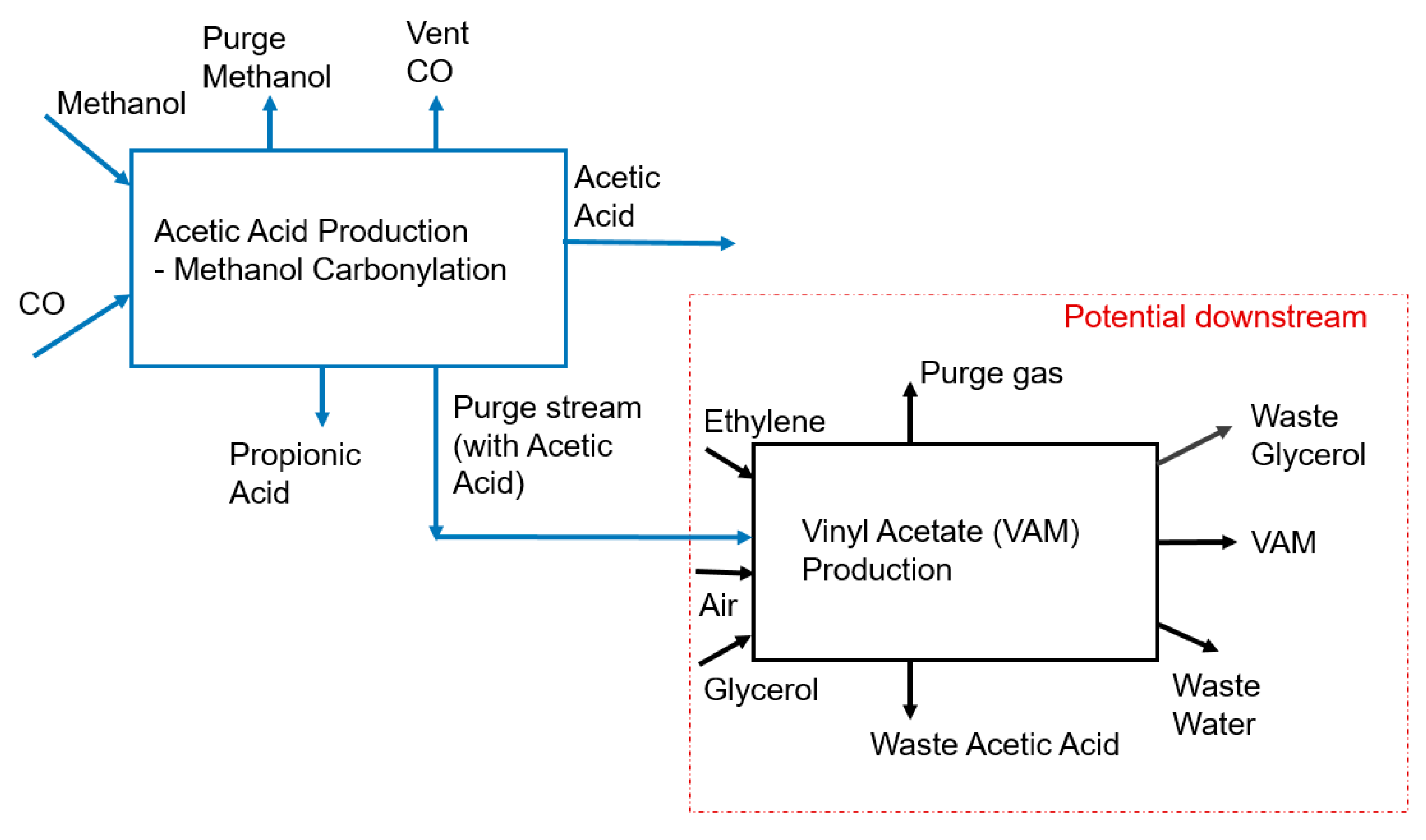
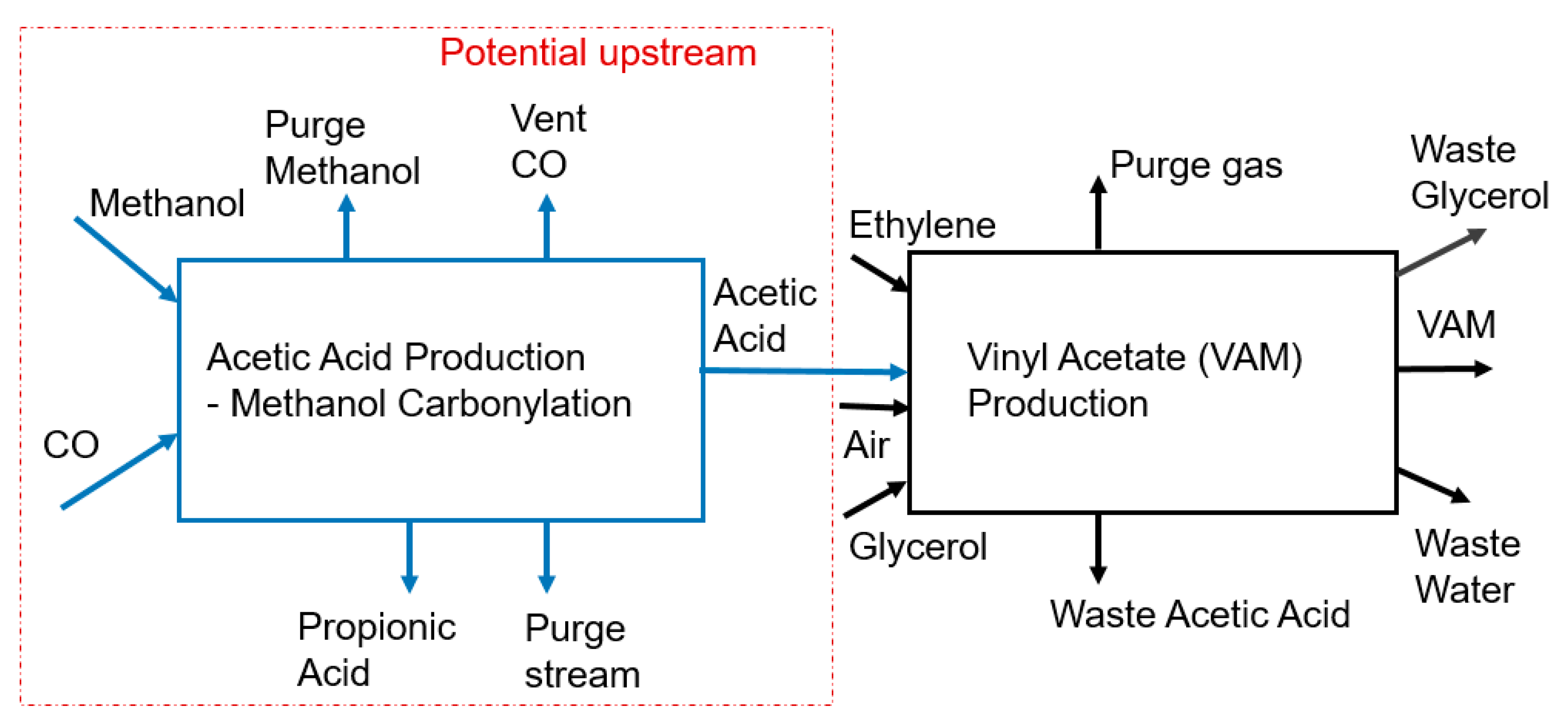
Two case studies from completely different industrial domains are provided which illustrate the applicability of the framework for the seamless assessment of the energy/exergy needs of the process systems. These include the processes of acetic acid production and MSW treatment areas.

The results from the first case study show that the separation and reuse of the acetic-acid-containing purge stream are exergy-prohibitive and that it is not probable that such a solution would be sustainable. The follow-up analysis of the acetic acid production shows that the process requires a substantial external exergy input. Determining the degree of sustainability of such a process needs further analysis of the possible sources of providing such exergy.

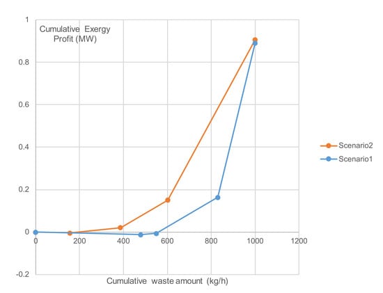
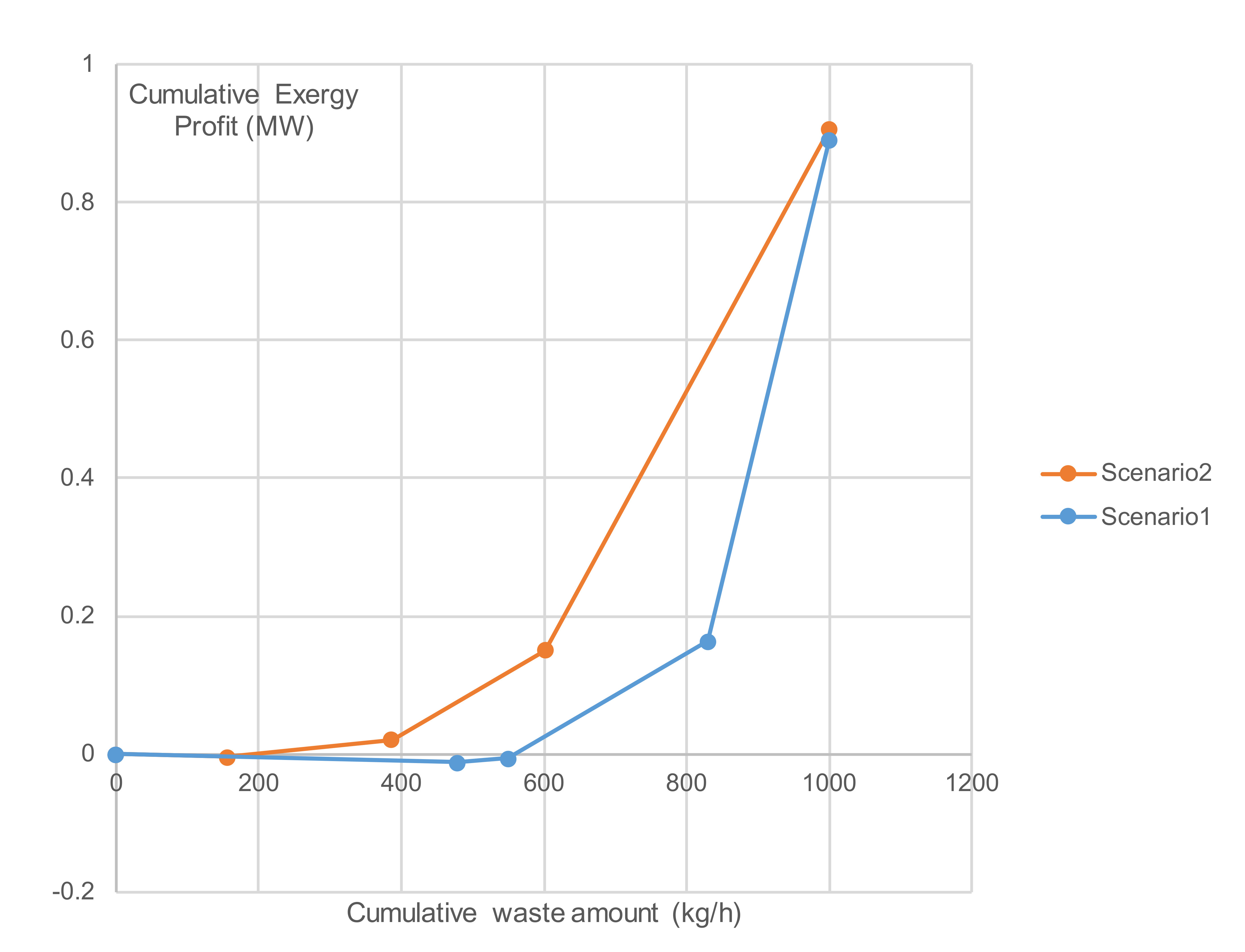
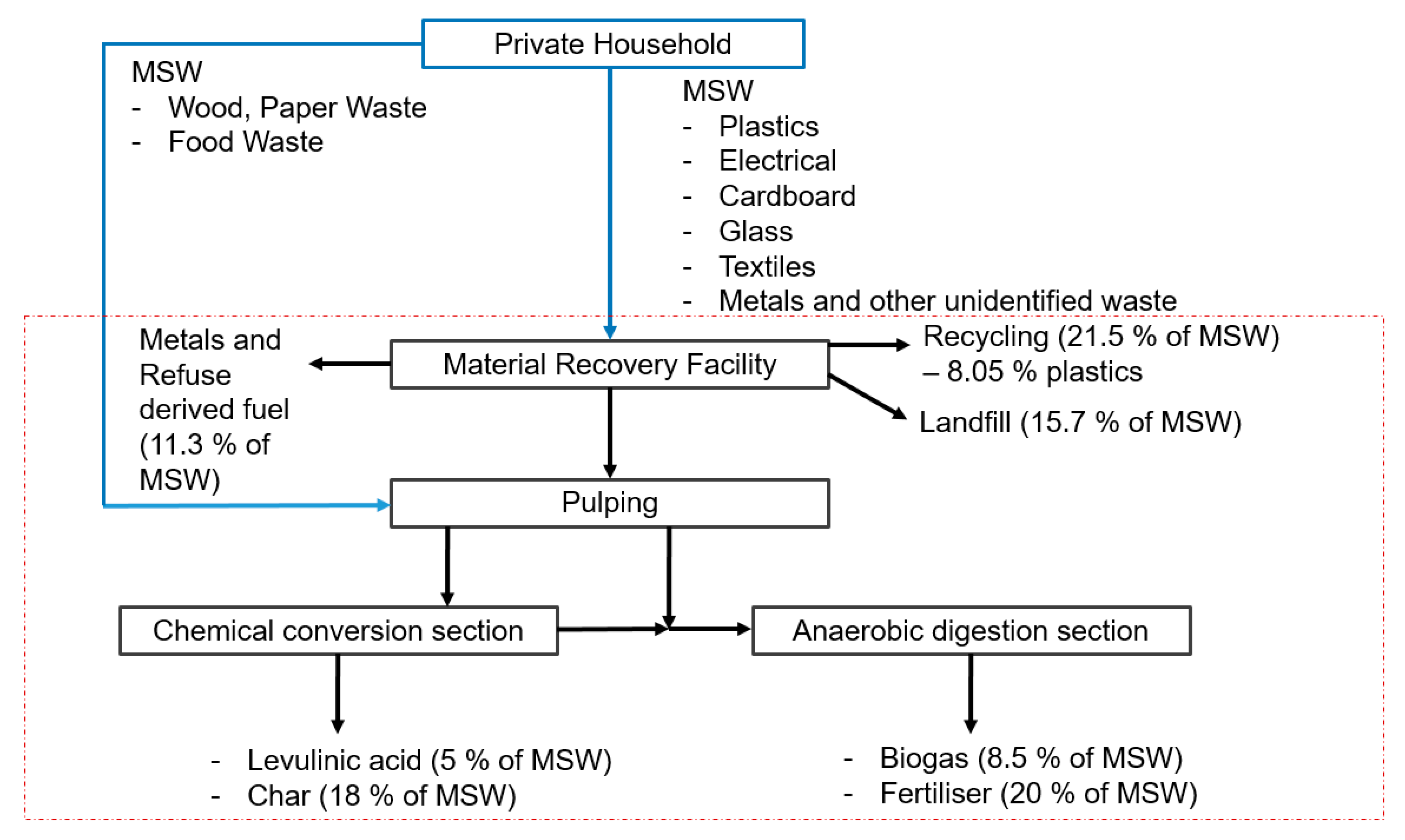
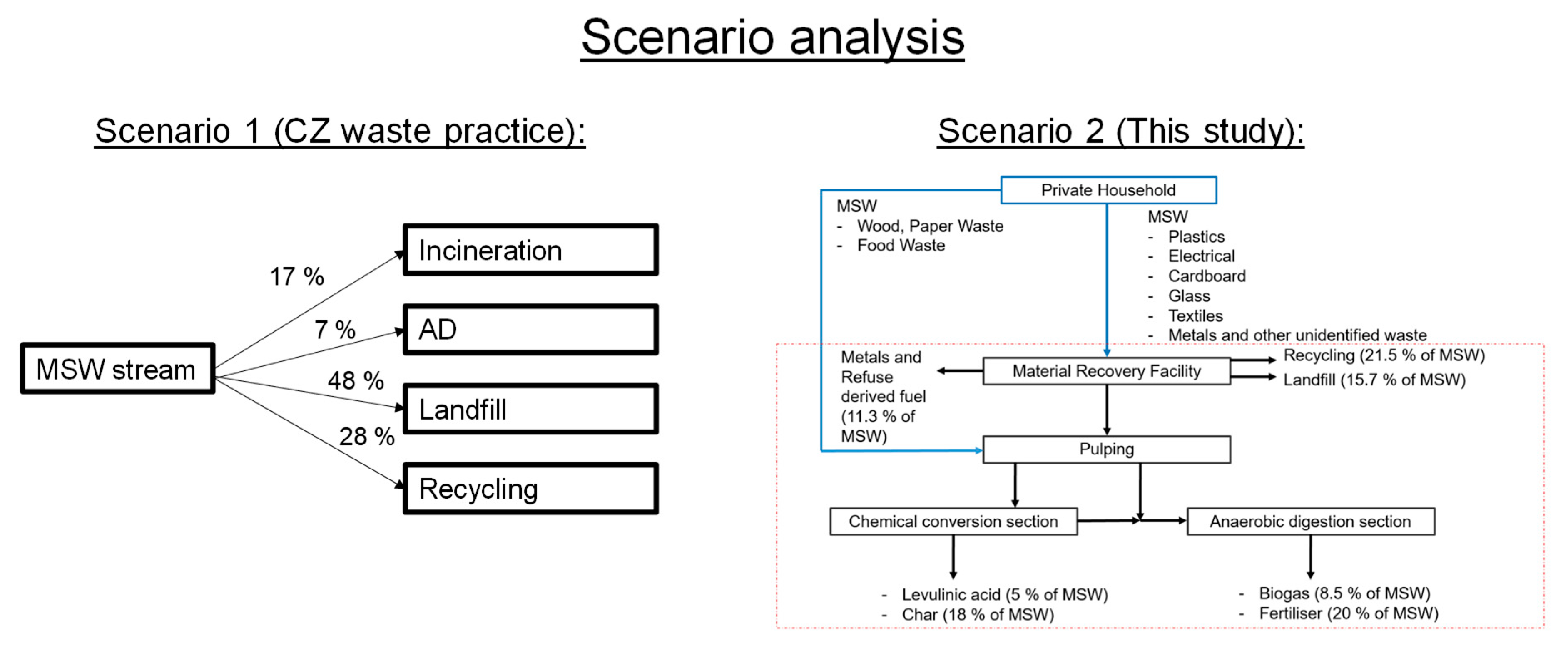
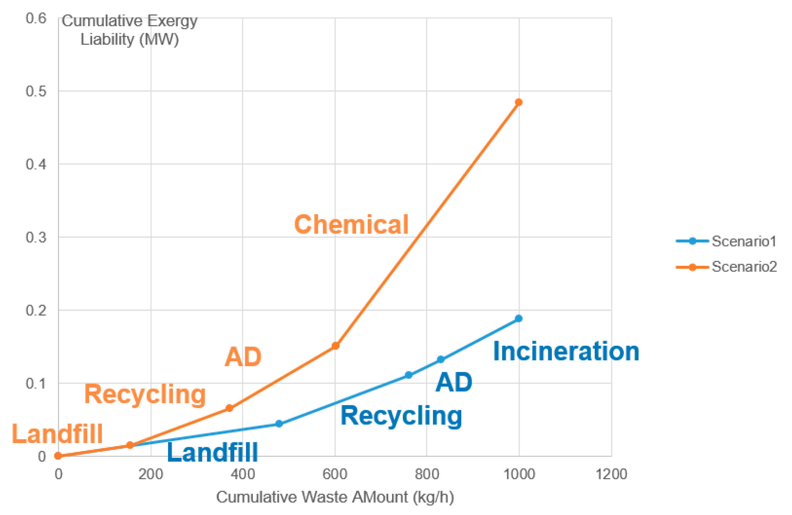
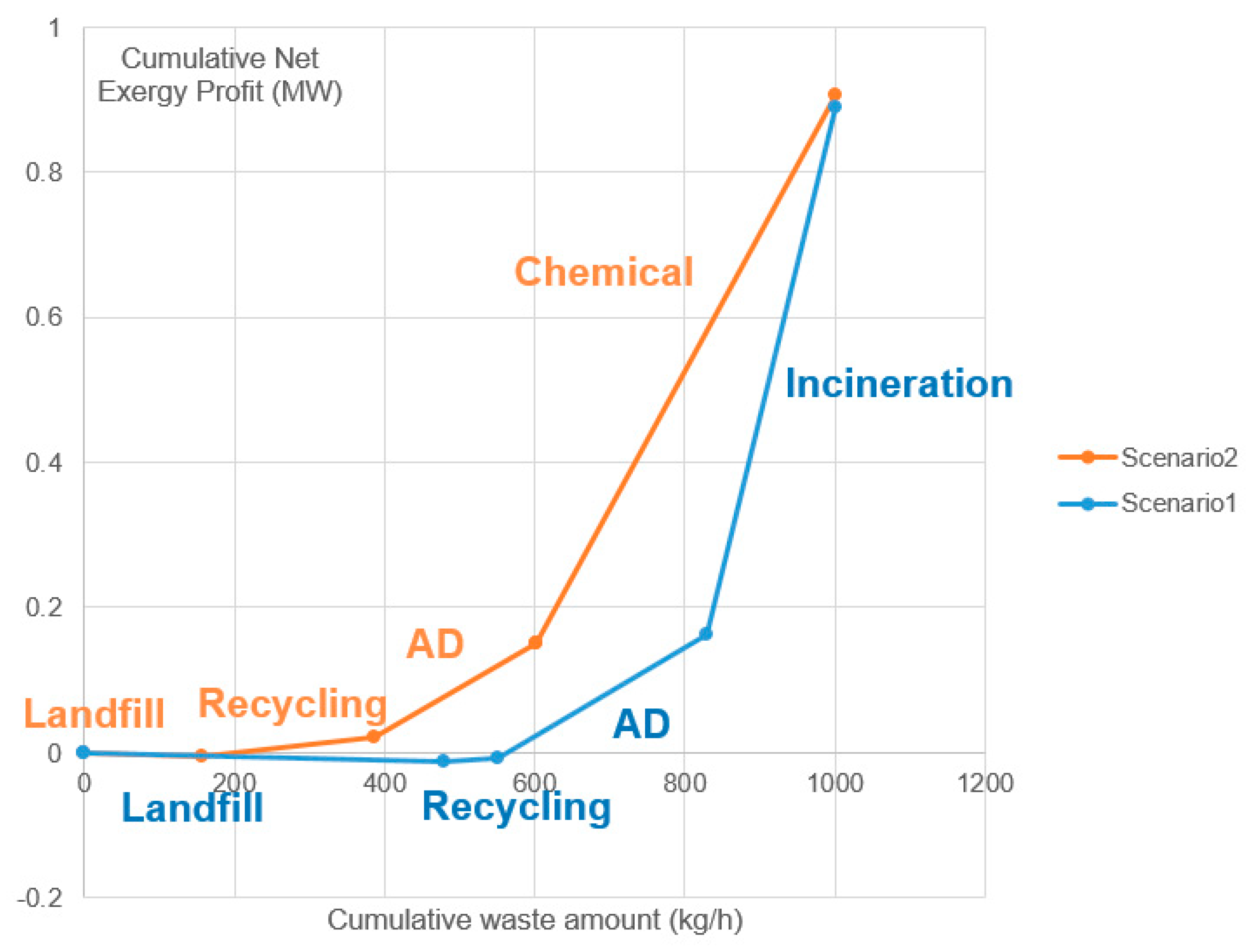
The second case study clearly shows the sustainability potential of the MSW treatment for obtaining either useful energy directly or first extracting useful chemicals before the waste-to-energy process. The developed cumulative Exergy Composite Curves show a marginal advantage (less than 10%) of the chemical extraction route over the direct waste-to-energy route. The developed curves demonstrate that the proposed framework represents a useful toolset for evaluating process systems and alternative solutions.

The proposed concept can be further developed to create a complete framework which is capable of accounting for the thermodynamic irreversibility of processes. This will help us to reach a deeper understanding of the exergy flows, storages and losses and their relation to process sustainability.

Building on this, future work should incorporate economic metrics into the evaluation, leading to a complete toolset accounting for both the technical and economic performance of the considered process systems. This will make the tools suitable for decision-making in real engineering projects and for use by process managers and potential investors.

The correct selection of the system boundaries for the analysis of exergy footprints is key to the practical applicability of the concept. Full Life Cycle Assessment requires the collection of a large amount of information, which sometimes depends on subjective considerations. In many cases, not all stages of the life cycle are really significant with respect to the chosen criteria. In this context, further work should also be directed towards embedding this accounting framework within the Life Cycle Assessment framework, allowing for the scalability of the concepts and their adaptation to the modelling contexts.

References

1. Klemeš, J.; Huisingh, D. Economic use of renewable resources, LCA, cleaner batch processes and minimising emissions and wastewater. J. Clean. Prod. 2008, 16, 159–163. [Google Scholar] [CrossRef]
2. Klemeš, J.J.; Varbanov, P.S.; Ocłoń, P.; Chin, H.H. Towards Efficient and Clean Process Integration: Utilisation of Renewable Resources and Energy-Saving Technologies. Energies 2019, 12, 4092. [Google Scholar] [CrossRef] [Green Version]
3. Gerbens-Leenes, P.W.; Hoekstra, A.Y.; Bosman, R. The blue and grey water footprint of construction materials: Steel, cement and glass. Water Resour. Ind. 2018, 19, 1–12. [Google Scholar] [CrossRef]
4. Fan, Y.V.; Perry, S.; Klemeš, J.J.; Lee, C.T. A review on air emissions assessment: Transportation. J. Clean. Prod. 2018, 194, 673–684. [Google Scholar] [CrossRef]
5. Bong, C.P.C.; Lim, L.Y.; Ho, W.S.; Lim, J.S.; Klemeš, J.J.; Towprayoon, S.; Ho, C.S.; Lee, C.T. A review on the global warming potential of cleaner composting and mitigation strategies. J. Clean. Prod. 2017, 146, 149–157. [Google Scholar] [CrossRef]
6. Ghannadzadeh, A.; Thery-Hetreux, R.; Baudouin, O.; Baudet, P.; Floquet, P.; Joulia, X. General methodology for exergy balance in ProSimPlus® process simulator. Energy 2012, 44, 38–59. [Google Scholar] [CrossRef] [Green Version]
7. Dinçer, İ.; Rosen, M. Exergy: Energy, Environment, and Sustainable Development; Elsevier: Amsterdam, The Netherlands, 2007; ISBN 978-0-08-044529-8. [Google Scholar]
8. Ehyaei, M.A.; Ahmadi, A.; Rosen, M.A. Energy, exergy, economic and advanced and extended exergy analyses of a wind turbine. Energy Convers. Manag. 2019, 183, 369–381. [Google Scholar] [CrossRef]
9. Song, D.; Lin, L.; Wu, Y. Extended exergy accounting for a typical cement industry in China. Energy 2019, 174, 678–686. [Google Scholar] [CrossRef]
10. Amiri, Z.; Asgharipour, M.R.; Campbell, D.E.; Armin, M. Extended exergy analysis (EAA) of two canola farming systems in Khorramabad, Iran. Agric. Syst. 2020, 180, 102789. [Google Scholar] [CrossRef]
11. Wan Alwi, S.R.; Manan, Z.A.; Klemeš, J.J.; Huisingh, D. Sustainability engineering for the future. J. Clean. Prod. 2014, 71, 1–10. [Google Scholar] [CrossRef]
12. Avraamidou, S.; Baratsas, S.G.; Tian, Y.; Pistikopoulos, E.N. Circular Economy-A challenge and an opportunity for Process Systems Engineering. J. Clean. Prod. 2020, 133, 106629. [Google Scholar] [CrossRef]
13. Dincer, I.; Rosen, M.A.; Al-Zareer, M. 5.5 Exergy Management. In Comprehensive Energy Systems; Dincer, I., Ed.; Elsevier: Amsterdam, The Netherlands, 2018; pp. 166–201. ISBN 978-0-12-814925-6. [Google Scholar]
14. Makarieva, A.M.; Gorshkov, V.G.; Li, B.-L. Energy budget of the biosphere and civilization: Rethinking environmental security of global renewable and non-renewable resources. Ecol. Complex. 2008, 5, 281–288. [Google Scholar] [CrossRef]
15. Gallegos-Muñoz, A.; Zaleta-Aguilar, A.; González-Rolón, B.; Rangel-Hernandez, V.H. On an Exergy Efficiency Definition of a Wastewater Treatment Plant. Int. J. Thermodyn. 2003, 6, 169–176. [Google Scholar]
16. Magnanelli, E.; Berglihn, O.T.; Kjelstrup, S. Exergy-based performance indicators for industrial practice. Int. J. Energy Res. 2018, 42, 3989–4007. [Google Scholar] [CrossRef] [Green Version]
17. Yamamoto, M.; Ishida, M. New Graphical Method for Representing Characteristic Features of Extraction. Ind. Eng. Chem. Res. 2002, 41, 277–284. [Google Scholar] [CrossRef]
18. Alotaibi, S.; Ibrahim, O.M.; Wang, Y.; Luo, T. Exergy Analysis of Directional Solvent Extraction Desalination Process. Entropy 2019, 21, 321. [Google Scholar] [CrossRef] [Green Version]
19. Zhang, J.; Qiao, Y.; Agar, D.W. Intensification of low temperature thermomorphic biphasic amine solvent regeneration for CO2 capture. Chem. Eng. Res. Des. 2012, 90, 743–749. [Google Scholar] [CrossRef]
20. Suh, S.; Lenzen, M.; Treloar, G.J.; Hondo, H.; Horvath, A.; Huppes, G.; Jolliet, O.; Klann, U.; Krewitt, W.; Moriguchi, Y.; et al. System Boundary Selection in Life-Cycle Inventories Using Hybrid Approaches. Environ. Sci. Technol. 2004, 38, 657–664. [Google Scholar] [CrossRef]
21. Szargut, J.; Valero, A.; Stanek, W.; Valero, A. Towards an International Reference Environment of Chemical Exergy. In Proceedings of the Conference ECOS 2005, Trondheim, Norway, 6 June 2005; pp. 409–420. [Google Scholar]
22. Szargut, J. International progress in second law analysis. Energy 1980, 5, 709–718. [Google Scholar] [CrossRef]
23. Szargut, J. Chemical exergies of the elements. Appl. Energy 1989, 32, 269–286. [Google Scholar] [CrossRef]
24. Gaudreau, K.; Fraser, R.A.; Murphy, S. The Characteristics of the Exergy Reference Environment and Its Implications for Sustainability-Based Decision-Making. Energies 2012, 5, 2197–2213. [Google Scholar] [CrossRef] [Green Version]
25. Valero, A.; Valero, A.; Stanek, W. Assessing the exergy degradation of the natural capital: From Szargut’s updated reference environment to the new thermoecological-cost methodology. Energy 2018, 163, 1140–1149. [Google Scholar] [CrossRef]
26. Ertesvåg, I.S. Sensitivity of chemical exergy for atmospheric gases and gaseous fuels to variations in ambient conditions. Energy Convers. Manag. 2007, 48, 1983–1995. [Google Scholar] [CrossRef]
27. Utlu, Z.; Hepbasli, A. Energetic and exergetic assessment of the industrial sector at varying dead (reference) state temperatures: A review with an illustrative example. Renew. Sustain. Energy Rev. 2008, 12, 1277–1301. [Google Scholar] [CrossRef]
28. Colombo, E.; Rocco, M.V.; Toro, C.; Sciubba, E. An exergy-based approach to the joint economic and environmental impact assessment of possible photovoltaic scenarios: A case study at a regional level in Italy. Ecol. Model. 2015, 318, 64–74. [Google Scholar] [CrossRef]
29. Cornelissen, R.L.; Hirs, G.G. The value of the exergetic life cycle assessment besides the LCA. Energy Convers. Manag. 2002, 43, 1417–1424. [Google Scholar] [CrossRef]
30. Dewulf, J.; Langenhove, H.V.; Mulder, J.; van den Berg, M.M.D.; van der Kooi, H.J.; de Arons, J.S. Illustrations towards quantifying the sustainability of technology. Green Chem. 2000, 2, 108–114. [Google Scholar] [CrossRef]
31. Michailos, S.; Parker, D.; Webb, C. Design, Sustainability Analysis and Multiobjective Optimisation of Ethanol Production via Syngas Fermentation. Waste Biomass Valor 2019, 10, 865–876. [Google Scholar] [CrossRef] [Green Version]
32. Quiroz-Ramírez, J.J.; Sánchez-Ramírez, E.; Segovia-Hernández, J.G. Energy, exergy and techno-economic analysis for biobutanol production: A multi-objective optimization approach based on economic and environmental criteria. Clean Techn. Environ Policy 2018, 20, 1663–1684. [Google Scholar] [CrossRef]
33. Leontief, W. The economy as a circular flow. Struct. Chang. Econ. Dyn. 1991, 2, 181–212. [Google Scholar] [CrossRef]
34. Nakajima, N. A Vision of Industrial Ecology: State-of-the-Art Practices for a Circular and Service-Based. Bull. Sci. Technol. Soc. 2000, 30, 54–69. [Google Scholar] [CrossRef]
35. Del Borghi, A.; Moreschi, L.; Gallo, M. Circular economy approach to reduce water–energy–food nexus. Curr. Opin. Environ. Sci. Health 2020, 13, 23–28. [Google Scholar] [CrossRef]
36. Hao, S.; Kuah, A.T.H.; Rudd, C.D.; Wong, K.H.; Lai, N.Y.G.; Mao, J.; Liu, X. A circular economy approach to green energy: Wind turbine, waste, and material recovery. Sci. Total Environ. 2020, 702, 135054. [Google Scholar] [CrossRef] [PubMed]
37. Fan, Y.V.; Klemeš, J.J.; Walmsley, T.G.; Bertók, B. Implementing Circular Economy in municipal solid waste treatment system using P-graph. Sci. Total Environ. 2020, 701, 134652. [Google Scholar] [CrossRef] [PubMed]
38. Manan, Z.A.; Nawi, W.N.R.M.; Alwi, S.R.W.; Klemeš, J.J. Advances in Process Integration research for CO2 emission reduction-A review. J. Clean. Prod. 2017, 167, 1–13. [Google Scholar] [CrossRef]
39. Smith, R. Chemical Process Design and Integration, 2nd ed.; Wiley: Hoboken, NJ, USA, 2016; ISBN 978-1-119-99014-7. [Google Scholar]
40. Korhonen, J.; Honkasalo, A.; Seppälä, J. Circular Economy: The Concept and its Limitations. Ecol. Econ. 2018, 143, 37–46. [Google Scholar] [CrossRef]
41. European Commission. Communication from the Commission to the European Parliament, The Council, The European Economic and Social Committee and the Committee of the Regions. Closing the Loop-An EU Action Plan for the Circular Economy COM/2015/0614 Final. Available online: https://eur-lex.europa.eu/resource.html?uri=cellar:8a8ef5e8-99a0-11e5-b3b7-01aa75ed71a1.0012.02/DOC_1&format=PDF (accessed on 5 January 2020).
42. Lieder, M.; Rashid, A. Towards circular economy implementation: A comprehensive review in context of manufacturing industry. J. Clean. Prod. 2016, 115, 36–51. [Google Scholar] [CrossRef]
43. Marrucci, L.; Daddi, T.; Iraldo, F. The integration of circular economy with sustainable consumption and production tools: Systematic review and future research agenda. J. Clean. Prod. 2019, 240, 118268. [Google Scholar] [CrossRef]
44. Pieroni, M.P.P.; McAloone, T.C.; Pigosso, D.C.A. Business model innovation for circular economy and sustainability: A review of approaches. J. Clean. Prod. 2019, 215, 198–216. [Google Scholar] [CrossRef]
45. Viegas, C.V.; Bond, A.; Vaz, C.R.; Bertolo, R.J. Reverse flows within the pharmaceutical supply chain: A classificatory review from the perspective of end-of-use and end-of-life medicines. J. Clean. Prod. 2019, 238, 117719. [Google Scholar] [CrossRef]
46. van der Wiel, B.Z.; Weijma, J.; van Middelaar, C.E.; Kleinke, M.; Buisman, C.J.N.; Wichern, F. Restoring nutrient circularity: A review of nutrient stock and flow analyses of local agro-food-waste systems. Resour. Conserv. Recycl. X 2019, 3, 100014. [Google Scholar] [CrossRef]
47. Gorman, M.R.; Dzombak, D.A. A review of sustainable mining and resource management: Transitioning from the life cycle of the mine to the life cycle of the mineral. Resour. Conserv. Recycl. 2018, 137, 281–291. [Google Scholar] [CrossRef]
48. Abadías Llamas, A.; Valero Delgado, A.; Valero Capilla, A.; Torres Cuadra, C.; Hultgren, M.; Peltomäki, M.; Roine, A.; Stelter, M.; Reuter, M.A. Simulation-based exergy, thermo-economic and environmental footprint analysis of primary copper production. Miner. Eng. 2019, 131, 51–65. [Google Scholar] [CrossRef]
49. Pinto, J.T.M.; Diemer, A. Supply chain integration strategies and circularity in the European steel industry. Resour. Conserv. Recycl. 2020, 153, 104517. [Google Scholar] [CrossRef]
50. Anastasiades, K.; Blom, J.; Buyle, M.; Audenaert, A. Translating the circular economy to bridge construction: Lessons learnt from a critical literature review. Renew. Sustain. Energy Rev. 2020, 117, 109522. [Google Scholar] [CrossRef]
51. Jarre, M.; Petit-Boix, A.; Priefer, C.; Meyer, R.; Leipold, S. Transforming the bio-based sector towards a circular economy-What can we learn from wood cascading? For. Policy Econ. 2020, 110, 101872. [Google Scholar] [CrossRef]
52. Haas, W.; Krausmann, F.; Wiedenhofer, D.; Heinz, M. How Circular is the Global Economy?: An Assessment of Material Flows, Waste Production, and Recycling in the European Union and the World in 2005. J. Ind. Ecol. 2015, 19, 765–777. [Google Scholar] [CrossRef]
53. European Commission. A European Strategy for Plastics in a Circular Economy. Available online: https://ec.europa.eu/environment/circular-economy/pdf/plastics-strategy-brochure.pdf (accessed on 5 January 2020).
54. Hahladakis, J.N.; Iacovidou, E. An overview of the challenges and trade-offs in closing the loop of post-consumer plastic waste (PCPW): Focus on recycling. J. Hazard. Mater. 2019, 380, 120887. [Google Scholar] [CrossRef]
55. Mesa, J.A.; Esparragoza, I.; Maury, H. Trends and Perspectives of Sustainable Product Design for Open Architecture Products: Facing the Circular Economy Model. Int. J. Precis. Eng. Manuf. Technol. 2019, 6, 377–391. [Google Scholar] [CrossRef]
56. Post, W.; Susa, A.; Blaauw, R.; Molenveld, K.; Knoop, R.J.I. A Review on the Potential and Limitations of Recyclable Thermosets for Structural Applications. Polym. Rev. 2019, 1–30. [Google Scholar] [CrossRef]
57. Corona, B.; Shen, L.; Reike, D.; Rosales Carreón, J.; Worrell, E. Towards sustainable development through the circular economy—A review and critical assessment on current circularity metrics. Resour. Conserv. Recycl. 2019, 151, 104498. [Google Scholar] [CrossRef]
58. 58 Sassanelli, C.; Rosa, P.; Rocca, R.; Terzi, S. Circular economy performance assessment methods: A systematic literature review. J. Clean. Prod. 2019, 229, 440–453. [Google Scholar] [CrossRef]
59. Saidani, M.; Yannou, B.; Leroy, Y.; Cluzel, F.; Kendall, A. A taxonomy of circular economy indicators. J. Clean. Prod. 2019, 207, 542–559. [Google Scholar] [CrossRef] [Green Version]
60. Tamura, S.; Fujie, K. Material Cycle of Agriculture on Miyakojima Island: Material Flow Analysis for Sugar Cane, Pasturage and Beef Cattle. Sustainability 2014, 6, 812–835. [Google Scholar] [CrossRef] [Green Version]
61. Pejpichestakul, W.; Siemanond, K. Process heat integration between distillation columns for ethylene hydration process. Chem. Eng. Trans. 2013, 35, 181–186. [Google Scholar]
62. Tsolas, S.D.; Karim, M.N.; Hasan, M.M.F. Optimization of water-energy nexus: A network representation-based graphical approach. Appl. Energy 2018, 224, 230–250. [Google Scholar] [CrossRef]
63. Tian, H.; Lu, C.; Pan, S.; Yang, J.; Miao, R.; Ren, W.; Yu, Q.; Fu, B.; Jin, F.-F.; Lu, Y.; et al. Optimizing resource use efficiencies in the food–energy–water nexus for sustainable agriculture: From conceptual model to decision support system. Curr. Opin. Environ. Sustain. 2018, 33, 104–113. [Google Scholar] [CrossRef]
64. Rulli, M.C.; Bellomi, D.; Cazzoli, A.; Carolis, G.D.; D’Odorico, P. The water-land-food nexus of first-generation biofuels. Sci. Rep. 2016, 6, 22521. [Google Scholar] [CrossRef] [Green Version]
65. Wang, X.-C.; Klemeš, J.J.; Dong, X.; Fan, W.; Xu, Z.; Wang, Y.; Varbanov, P.S. Air pollution terrain nexus: A review considering energy generation and consumption. Renew. Sustain. Energy Rev. 2019, 105, 71–85. [Google Scholar] [CrossRef]
66. Ewijk, S.V.; Stegemann, J.A.; Ekins, P. Global Life Cycle Paper Flows, Recycling Metrics, and Material Efficiency. J. Ind. Ecol. 2018, 22, 686–693. [Google Scholar] [CrossRef] [Green Version]
67. Awasthi, A.K.; Li, J. An overview of the potential of eco-friendly hybrid strategy for metal recycling from WEEE. Resour. Conserv. Recycl. 2017, 126, 228–239. [Google Scholar] [CrossRef]
68. Xue, M.; Kendall, A.; Xu, Z.; Schoenung, J.M. Waste Management of Printed Wiring Boards: A Life Cycle Assessment of the Metals Recycling Chain from Liberation through Refining. Environ. Sci. Technol. 2015, 49, 940–947. [Google Scholar] [CrossRef] [PubMed]
69. Balmer, R.T. Modern Engineering Thermodynamics; Academic Press: Cambridge, MA, USA, 2011; ISBN 978-0-12-374996-3. [Google Scholar]
70. Forman, C.; Muritala, I.K.; Pardemann, R.; Meyer, B. Estimating the global waste heat potential. Renew. Sustain. Energy Rev. 2016, 57, 1568–1579. [Google Scholar] [CrossRef]
71. European Commission. Statistical Office of the European Union Circular Material Use Rate: Calculation Method: 2018 Edition; Eurostat, European Commission: Brussels, Belgium, 2018; ISBN 978-92-79-96698-9. [Google Scholar]
72. Directive, E.U.W. EC Council Directive of 21 May 1991 concerning urban waste-water treatment. Off. J. Eur. Communities 1991, 34, 40–52. [Google Scholar]
73. High Temperature-King County. Available online: https://www.kingcounty.gov/services/environment/wastewater/industrial-waste/limits-regulations/limits-prohibited/high-temperature.aspx (accessed on 14 December 2019).
74. Turner, T. Effluent Standards; UN FAO, 2019; p. 16. Available online: https://oaout.epa.gov.tw/law/Download.ashx?FileID=851 (accessed on 14 December 2019).
75. Klemeš, J.J. (Ed.) Assessing and Measuring Environmental Impact and Sustainability; Butterworth-Heinemann/Elsevier: Oxford, UK, 2015; ISBN 978-0-12-799968-5. [Google Scholar]
76. Szargut, J.; Morris, D.R.; Steward, F.R. Exergy Analysis of Thermal, Chemical, and Metallurgical Processes; Hemisphere: New York, NY, USA, 1988. [Google Scholar]
77. Chemical Exergy Calculator—The Exergoecology Portal. Available online: www.exergoecology.com/excalc (accessed on 28 December 2019).
78. Berre, C.L.; Serp, P.; Kalck, P.; Torrence, G.P. Acetic Acid. In Ullmann’s Encyclopedia of Industrial Chemistry; American Cancer Society: Atlanta, GA, USA, 2014; pp. 1–34. ISBN 978-3-527-30673-2. [Google Scholar]
79. Dimian, A.C.; Bildea, C.S.; Kiss, A.A. Acetic Acid. In Applications in Design and Simulation of Sustainable Chemical Processes; Elsevier: Amsterdam, The Netherlands, 2019; pp. 483–519. ISBN 978-0-444-63876-2. [Google Scholar]
80. Galli, F.; Previtali, D.; Casagrande, S.; Pirola, C.; Manenti, F.; Boffito, D.C. Simulation of the Water-Acetic Acid Separation via Distillation Using Different Entrainers: An Economic Comparison. Chem. Eng. Trans. 2017, 57, 1159–1164. [Google Scholar]
81. Langell, M.A.; Berrie, C.L.; Nassir, M.H.; Wulser, K.W. Adsorption of acetic acid on hydroxylated NiO(111) thin films. Surf. Sci. 1994, 320, 25–38. [Google Scholar] [CrossRef]
82. Aspen HYSYS. Available online: https://www.aspentech.com/en/products/engineering/aspen-hysys (accessed on 21 November 2019).
83. Contreras, J.P.; Naranjo, J.C.G.; Ramírez, S.G.; Martinez, D.M. Vinyl Acetate from ethylene, acetic acid and oxygen Industrial Plant Simulation. In Proceedings of the Computing and Systems Technology Division, American Institute of Chemical Engineers (AIChE) Annual Meeting, Nashville, TN, USA, 10–15 November 2009; pp. 249–259. [Google Scholar]
84. Sadhukhan, J.; Ng, K.S.; Martinez-Hernandez, E. Novel integrated mechanical biological chemical treatment (MBCT) systems for the production of levulinic acid from fraction of municipal solid waste: A comprehensive techno-economic analysis. Bioresour. Technol. 2016, 215, 131–143. [Google Scholar] [CrossRef]
85. Bhaskar, T.; Steele, P.H. Thermo-chemical Conversion of Biomass. Bioresour. Technol. 2015, 178, 1. [Google Scholar] [CrossRef]
86. Batalha, L.A.R.; Han, Q.; Jameel, H.; Chang, H.; Colodette, J.L.; Borges Gomes, F.J. Production of fermentable sugars from sugarcane bagasse by enzymatic hydrolysis after autohydrolysis and mechanical refining. Bioresour. Technol. 2015, 180, 97–105. [Google Scholar] [CrossRef]
87. Ferdan, T.; Pavlas, M.; Šomplák, R.; Nevrlý, V.; Klemeš, J.J.; Pitschke, T. Allocation analysis of waste treatment nodes for economic optimisation considering reduced greenhouse gas emissions. Chem. Eng. Trans. 2017, 61, 967–972. [Google Scholar]
88. Pan, Z.; Chan, W.P.; Veksha, A.; Giannis, A.; Dou, X.; Wang, H.; Lisak, G.; Lim, T.-T. Thermodynamic analyses of synthetic natural gas production via municipal solid waste gasification, high-temperature water electrolysis and methanation. Energy Convers. Manag. 2019, 202, 112160. [Google Scholar] [CrossRef]
89. Yang, Y.; Heaven, S.; Venetsaneas, N.; Banks, C.J.; Bridgwater, A.V. Slow pyrolysis of organic fraction of municipal solid waste (OFMSW): Characterisation of products and screening of the aqueous liquid product for anaerobic digestion. Appl. Energy 2018, 213, 158–168. [Google Scholar] [CrossRef]
90. Licari, A.; Monlau, F.; Solhy, A.; Buche, P.; Barakat, A. Comparison of various milling modes combined to the enzymatic hydrolysis of lignocellulosic biomass for bioenergy production: Glucose yield and energy efficiency. Energy 2016, 102, 335–342. [Google Scholar] [CrossRef]
91. Mukherjee, A.; Dumont, M.-J.; Raghavan, V. Review: Sustainable production of hydroxymethylfurfural and levulinic acid: Challenges and opportunities. Biomass Bioenergy 2015, 72, 143–183. [Google Scholar] [CrossRef]
92. Fodor, Z.; Klemeš, J.J. Waste as alternative fuel–Minimising emissions and effluents by advanced design. Process Saf. Environ. Prot. 2012, 90, 263–284. [Google Scholar] [CrossRef]
93. Eboh, F.C.; Ahlström, P.; Richards, T. Estimating the specific chemical exergy of municipal solid waste. Energy Sci. Eng. 2016, 4, 217–231. [Google Scholar] [CrossRef] [Green Version]
94. Dewulf, J.; Langenhove, H.V. Thermodynamic optimization of the life cycle of plastics by exergy analysis. Int. J. Energy Res. 2004, 28, 969–976. [Google Scholar] [CrossRef]
95. Fan, Y.V.; Klemeš, J.J.; Chin, H.H. Extended Waste Management Pinch Analysis (E-WAMPA) Minimising Emission of Waste Management: EU 28. Chem. Eng. Trans. 2019, 74, 283–288. [Google Scholar]
96. Wu, Y.; Yang, W.; Blasiak, W. Energy and Exergy Analysis of High Temperature Agent Gasification of Biomass. Energies 2014, 7, 2107–2122. [Google Scholar] [CrossRef]
97. Dincer, I.; Rosen, M.A. Chapter 21-Exergy Analysis of Countries, Regions, and Economic Sectors. In Exergy, 2nd ed.; Dincer, I., Rosen, M.A., Eds.; Elsevier: Amsterdam, The Netherlands, 2013; pp. 425–450. ISBN 978-0-08-097089-9. [Google Scholar]
Figure 1. A multi-input–output process for an example of an agriculture system.
Energies 13 02132 g001
Figure 2. Ethanol production from ethylene summarised from the example in [61].
Energies 13 02132 g002
Figure 3. Global material cycles.
Energies 13 02132 g003
Figure 4. Energy cascading; data extracted from [70]. PV: photovoltaics.
Energies 13 02132 g004
Figure 5. Procedure for assigning exergy assets and liabilities.
Energies 13 02132 g005
Figure 6. Exergy profit evaluation of waste acetic acid stream.
Energies 13 02132 g006
Figure 7. Aspen HYSYS simulation flowsheet of vinyl acetate production, adapted from [83]. AA: acetic acid.
Energies 13 02132 g007
Figure 8. Exergy profit evaluation of inlet acetic acid stream.
Energies 13 02132 g008
Figure 9. Mechanical biological chemical treatment (MBCT) of Municipal Solid Waste (MSW), with mass balances between input and output,), adapted from [84].
Energies 13 02132 g009
Figure 10. Workflows for MSW treatment under comparison.
Energies 13 02132 g010
Figure 11. Composite Curves for the exergy liabilities of the MSW treatment under comparison.
Energies 13 02132 g011
Figure 12. Composite Curves for the exergy profit of the MSW treatment under comparison.
Energies 13 02132 g012