The Role of Biorefinery Co-Products, Market Proximity and Feedstock Environmental Footprint in Meeting Biofuel Policy Goals for Winter Barley-to-Ethanol

Abstract

Renewable fuel standards for biofuels have been written into policy in the U.S. to reduce the greenhouse gas (GHG) intensity of transportation energy supply. Biofuel feedstocks sourced from within a regional market have the potential to also address sustainability goals. The U.S. Mid-Atlantic region could meet the advanced fuel designation specified in the Renewable Fuel Standard (RFS2), which requires a 50% reduction in GHG emissions relative to a gasoline baseline fuel, through ethanol produced from winter barley (Hordeum vulgare L.). We estimate technology configurations and winter barley grown on available winter fallow agricultural land in six Mid-Atlantic states. Using spatially weighted stochastic GHG emission estimates for winter barley supply from 374 counties and biorefinery data from a commercial dry-grind facility design with multiple co-products, we conclude that winter barley would meet RFS2 goals even with the U.S. EPA’s indirect land use change estimates. Using a conservative threshold for soil GHG emissions sourced from barley produced on winter fallow lands in the U.S. MidAtlantic, a biorefinery located near densely populated metropolitan areas in the Eastern U.S. seaboard could economically meet the requirements of an advanced biofuel with the co-production of CO₂ for the soft drink industry.

1. Introduction

Much has been written, debated, and recast over what constitutes a “green” or environmentally sustainable biofuel. The development of renewable and low carbon fuel standards has shaped the way in which life cycle assessment (LCA) tools are used to judge a fuel’s “greenness,” specifically for addressing greenhouse gas (GHG) mitigation [1]. For example, LCA methods dictate choice of temporal, spatial, and process boundary selection [2,3], and treatment of co-products [4,5]. Crop-based fuels such as ethanol derived from corn have come under scrutiny for disrupting food markets and for the risks they pose towards indirect deforestation and carbon emissions, known as indirect land use change (iLUC) [6,7]. This is because the starch-based crops used to produce ethanol via wet or dry milling processes are grown on prime agricultural lands that compete with food, and thereby disrupt food prices. However, recent studies have shown the penalty of iLUC to be small yet complex when grains like corn and soybean are traded in global markets [8]. Ways of lessening or circumventing the iLUC CO₂ “penalty” include using waste or growing energy crops, whether starch or lignocellulosic, on marginal lands, or growing those crops when land has been historically fallow. Winter double-cropping can make use of fallow land because in certain agricultural regions it is seldom economical to grow winter crops (e.g., winter wheat) for food or feed, and historic records show that farmers have left the land fallow.

If a winter crop used for energy does not disrupt summer crop yield in a rotation, the indirect CO₂ penalty may be minimized. Furthermore, when winter double crops are grown using best management practices (BMP) such as conservation tillage and with optimized nitrogen fertilizer application, they may provide water quality benefits through reducing the NO₃ leaching and runoff from agricultural fields [9] that contribute to seasonal hypoxic zones [10]. Jayasundara et al. [11] reported improved fertilizer uptake efficiency and reduced gaseous and leached losses of NO₃–N through incorporating BMPs in corn–soybean–winter wheat rotations in Ontario, Canada. Therefore, winter small grains such as barley could, in the interim while lignocellulose-based fuel technologies mature, be promising agricultural feedstocks for low carbon fuels that promote energy security and rural economic development—ingredients necessary for deeming a fuel “sustainable.”

A suite of biofuels derived from non-corn starch-based feedstocks converted to ethanol that meet a 50% reduction in life cycle GHG emissions relative to gasoline could meet the advanced fuels designation under the Renewable Fuel Standard (RFS2) of the Energy Independence and Security (EISA) Act of 2007 [12]. Barley-to-ethanol produced under select operating conditions was proposed by the U.S. Environmental Protection Agency (EPA) as a renewable and advanced biofuel [13] as was grain sorghum-to-ethanol [14]. In the U.S. Mid-Atlantic region and surrounding states that could support winter cropping (Virginia, North Carolina, Maryland, Delaware, Pennsylvania, and Kentucky), barley (Hordeum vulgare L.) can be grown as a winter double-crop. Other double-crops like camelina (Camelina sativa L.) and field pennycress (Thlaspi arvense L.) oilseeds have been proposed as feedstock for biofuel that can provide ecosystem services if integrated into corn–soybean crop rotations [15]. For example, Krohn and Fripp [16] estimate that biodiesel made from spring camelina grown as a double crop achieved a 40% to 60% reduction in life cycle GHGs, assuming no iLUC effects. Tabatabaie et al. examined soil parameters affecting camelina as a winter crop for biodiesel production in Western U.S. states to estimate multiple life cycle impact assessment (LCIA) metrics [17].

Starch-based cereal grains such as barley [18], wheat (Triticum aestivum L.) [19], and sorghum (Sorghum bicolor (L.) Moench) [20] can be converted to ethanol using commercial technology. In most cases, results from technoeconomic analyses (TEA) have concluded that stable or low feedstock costs along with rising fossil fuel prices are needed to render grain alcohol competitive. Additionally, value-added co-products can improve biorefinery economics. Environmental life cycle assessments have been undertaken for agricultural commodities like barley grain [21] and straw [22], and for ethanol produced from grain sorghum [23], wheat [24], and cellulosic feedstocks [25] to understand the life cycle impacts related to global warming, eutrophication and acidification potential. To date, LCA of winter barley grain as a feedstock to produce ethanol has not been studied.

Malca and Freire [24] examined uncertainties in life cycle GHG emissions for wheat-to-ethanol in Europe, and showed that the highest and most variable GHG emissions related first to soil organic carbon (SOC), and second to nitrous oxide emissions during crop production. The contribution of SOC to the life cycle of crops strongly depends on the land use history of the growing region as noted in previous biofuel research [23,26,27,28]; thus, it is best modeled using Tier 3 IPCC (Intergovernmental Panel on Climate Change) biogeochemical or process models to predict the consequences of SOC and N₂O emissions when winter crops are introduced into a rotation. Tier 3 methods have been used to predict soil N₂O emissions to understand policy compliance for barley in advanced biofuel and low carbon fuel standard policy frameworks [29]. The biogeochemical models used in Tier 3 approaches require many detailed input parameters that cannot be known precisely. To address this uncertainty, Gao et al. [29] explored the use of a “margin of safety” approach in which emissions estimates are based not on the central tendency of model results, but on plausible upper bounds, such that one can have confidence that actual emissions will in all likelihood be lower than the estimated value (see Springborn et al. [30] for a discussion of the theoretical basis of margin of safety approaches).

The overall objective of this paper is to evaluate the environmental conditions for meeting advanced fuel designation for biofuels produced within the vicinity of high population centers on the U.S. East Coast using regionally available winter barley and commercial dry-grind technology. Using a life cycle modeling approach, we investigate alternative co-product scenarios and policy implications for meeting the advanced fuel designation in the Mid-Atlantic region of the U.S. using winter barley in corn (Zea mays L.)–soybean (Glycine max L.) rotations through examination of attributional and consequential LCA approaches and uncertainty. Prior research has used LCA with Monte Carlo simulation to understand the sources and effects of uncertain model parameters on GHG emissions in grain [24,31] and lignocellulosic feedstocks and technology [32] used to produce ethanol transport fuel. Moreover, LCA studies have demonstrated the importance of biomass logistics and scale [33,34,35], spatial aspects [36], and uncertainty [37] in feedstock supply to biorefineries on life cycle environmental impacts. We investigate the role of biorefinery proximity to end-markets for co-products in relation to meeting RFS2 advanced biofuel policy requirements, while considering the uncertainty in soil GHG emissions in the winter barley-to-ethanol (WBE) life cycle using Monte Carlo methods. We compare WBE to grain sorghum-to-ethanol, also a starch-based fuel substitute for gasoline to compare each pathway’s compliance with RFS2.

2. Materials and Methods

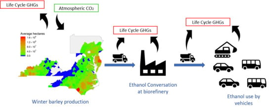
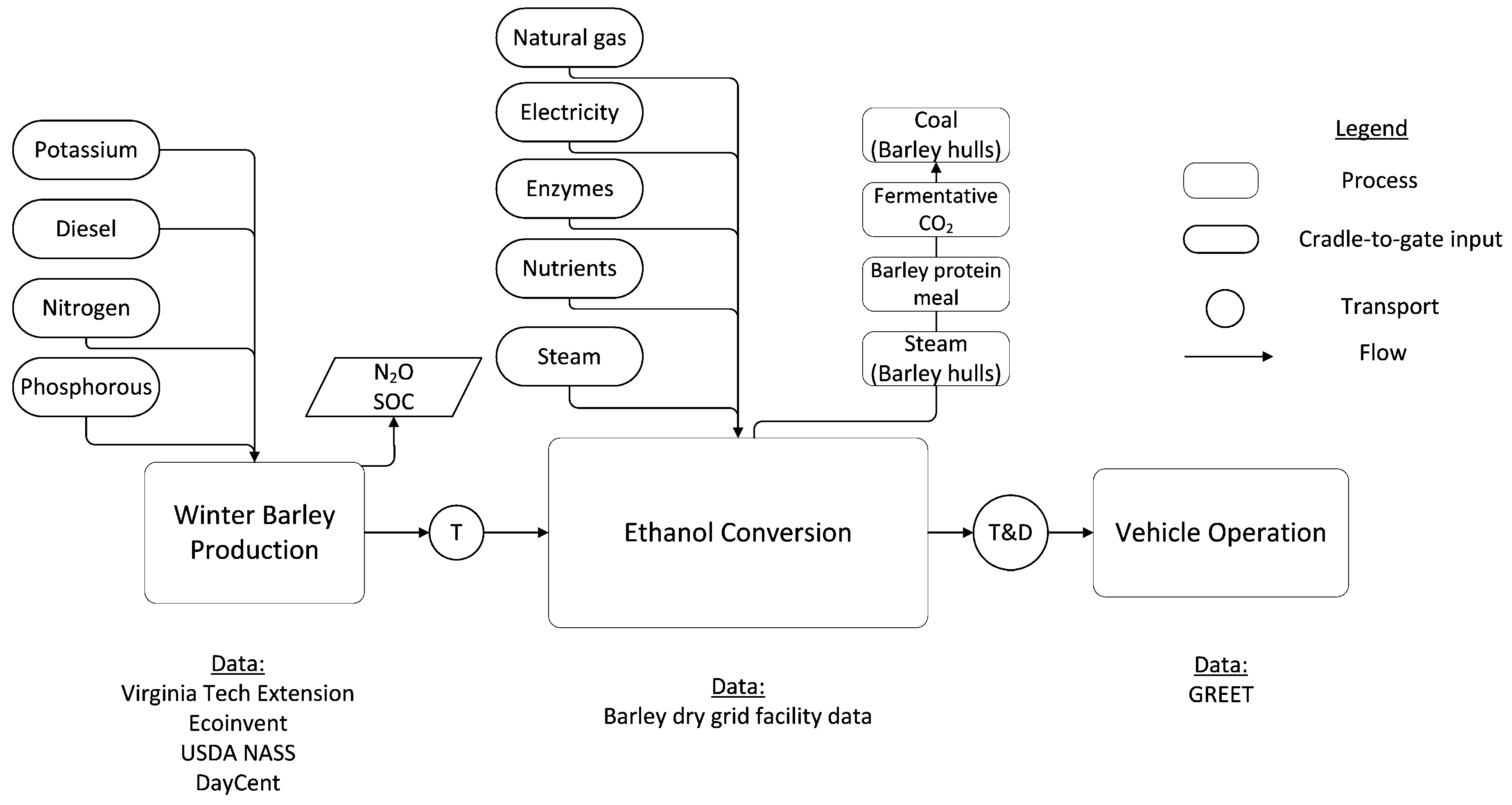
2.1. System Boundary Definition

We use life cycle assessment (LCA) following ISO standards [38] to evaluate scenarios for meeting the advanced fuel designation under RFS2 policy in the U.S. Mid-Atlantic region. We focus on two LCIA metrics, the 100-year global warming potential (GWP) to examine RFS2 policy compliance and cumulative energy demand (CED), a metric that measures renewable and nonrenewable energy inputs in a product life cycle and is relevant to evaluating proposed renewable fuel pathways as studied in prior bioenergy systems [39,40]. Criteria specified by the U.S. EPA for meeting advanced fuel standing require that a non-corn feedstock fuel’s life cycle GHG emissions be 50% lower than the 2005 gasoline baseline, which is set to 93 g CO₂e MJ⁻¹. We evaluate winter barley grown in six states (Figure 1) that could supply the Mid-Atlantic market under four biorefinery scenarios (

Table 1. Winter barley-to-ethanol (WBE) production scenarios with alternative co-product crediting examined through attributional LCA (life cycle assessment) boundary.

Scenario	Major Assumptions
WBE1	Biorefinery includes co-product crediting for:
	fermentative CO2 capture for the beverage industry;
	barley protein meal;
	onsite steam production;
	barley hull waste pelleting for cofiring with coal for power generation.
WBE2	Biorefinery includes co-product crediting for:
	barley protein meal;
	onsite steam production;
	barley hull waste pelleting for cofiring with coal for power generation.
WBE3	Biorefinery includes the production of co-products (barley protein meal, onsite steam production, and barley hull waste pelleting for coal cofiring). A co-product credit is only assigned to the barley protein meal.
WBE4	Biorefinery includes the production of three co-products (barley protein meal, onsite steam production, and barley hull waste pelleting for coal cofiring). No credits are applied for the avoided co-products.

) that include up to four co-products. The system boundary (Figure 2) includes all processes for growing, harvesting, and transporting winter barley grain to the biorefinery, conversion to ethanol and co-products, transporting, and distributing the fuel, and consuming the fuel. The functional unit defined is 1 MJ of denatured ethanol product (E98). We evaluate GHG emissions using the 100-year global warming potential (GWP) where CO₂, CH₄, and N₂O have a GWP of 1, 25, and 298 g CO₂ equivalents (CO₂e), respectively, based on the IPCC’s fourth Assessment Report (AR4) [41].

Winter barley is typically planted in late October to early November and harvested in late May to mid-June. In the Mid-Atlantic region, the most widely deployed acres are fallow during winter of the two-year corn and soybean rotation. Farmers in the Chesapeake Bay watershed have grown winter cover and double crops through incentive programs to reduce nutrient leaching for many years. Moreover, agricultural crops, including winter double crops and lignocellulosic feedstocks have been proposed as strategies for reducing nutrient and sediment runoff from farm fields, thereby improving the water quality of the Chesapeake Bay [42]. Thus, winter double-crops such as winter barley may be environmentally and socioeconomically attractive to growers in the Mid-Atlantic region since adding them to the agricultural landscape could improve water quality and create economic opportunities for growers, while also meeting EISA policy objectives.

The technology used to convert winter barley to ethanol [18] is similar to commercial corn dry-grind milling [43,44], which produces a fuel (ethanol), a protein co-product (barley protein), and in the case of winter barley, energetic and chemical commodities from the barley hulls and fermentative CO₂, respectively. The ethanol biorefinery for this study was based on a 245 million liter per year facility that was under construction between 2010 and 2011 by the company Osage Bio Energy in Hopewell, Virginia, near the Richmond metropolitan area. In addition to fuel ethanol, the biorefinery was designed to co-produce barley protein meal, process steam from barley hulls, and food-grade fermentative CO₂ for the beverage industry, all value-added products that improve biorefinery economics and life cycle environmental performance (Table 1).

2.2. Life Cycle Inventory Analysis

Data for constructing the life cycle inventory (LCI) model include crop production, transportation of the feedstock to the biorefinery, fuel conversion, transportation and distribution of denatured ethanol, and the combustive emissions for using the fuel. The LCI model was constructed using SimaPro 8.4 [45] with agronomic inputs specified by Thomason [46], nitrous oxide emissions and changes in soil organic carbon (SOC) generated using the DayCent model [47], process–guarantee data from a starch-based biorefinery completed in Hopewell, Virginia, in 2011, and vehicle in-use emissions from the GREET 1 model [48]. Uncertainty in the most sensitive parameter inputs were considered and integrated into the LCI model using Monte Carlo simulation.

2.2.1. Feedstock Production

To support a 245 million liter ethanol facility in the Mid-Atlantic U.S. winter barley can be grown on available annual winter fallow land ranging from 158,000 to 195,000 ha in Virginia, North Carolina, Maryland, and Delaware, and thus support 0.68 million dry metric tons year⁻¹ (31.3 million bushels year⁻¹) of winter barley. We also consider available winter fallow land in Pennsylvania and Kentucky (Figure 1). The winter crop is planted in October (following corn) and harvested in mid and late June (prior to soybean) in a two-year rotation using reduced tillage methods. U.S. Department of Agriculture (USDA) crop acreage data from 2008 [49] were evaluated to estimate fallow land available within a 80 and 160 km radius of the proposed Hopewell, Virginia, biorefinery. Between 0.74 and 1.47 million dry metric tons of winter barley could be grown on winter fallow lands within the existing corn, soybean, hay, and converted tobacco croplands.

The LCI includes addition of N, P, and K nutrients, and energy for field preparation and feedstock harvesting. Preharvest nutrient additions described by Thomason [46] specify a winter barley yield of 5380 kg ha⁻¹ and application of fertilizers in the following proportions: nitrogen (N), preplant urea (12 kg N ha⁻¹) and spring liquid urea ammonium nitrate (70 kg N ha⁻¹); phosphate (P), diammonium phosphate (23 kg N ha⁻¹, 58 kg P ha⁻¹); potassium, (52 kg K ha⁻¹); and lime (0.74 metric tons ha⁻¹). Lubricant, oil, and diesel fuel inputs are applied in preharvest (12.7 L diesel ha⁻¹) and in harvest (16.9 L diesel ha⁻¹) portions. Addition of herbicides are low and deemed to be outside of the cutoff criteria for the system boundary and their respective emissions were not analyzed.

2.2.2. Winter Barley Soil GHG Emissions

We estimate N₂O and SOC GHG emissions resulting from the introduction of winter barley on existing winter fallow land in six states (Virginia, North Carolina, Maryland, Delaware, Pennsylvania, and Kentucky). These states represent a feedstock supply radius larger than the 80 to 160 km radius of Hopewell, Virginia. The goal of selecting a wider winter barley growing region was to capture a larger extent of soil and climate region, which influences N₂O emissions and SOC. N₂O is emitted from agricultural soils directly to air through the process of nitrification/denitrification, and also indirectly following leaching into nearby water sources and reaction of NOx, NH₃, and water. With the exception of a few studies [23,27,50,51], much prior grain-to-alcohol LCA literature (e.g., Hsu et al. [31] and Wang et al. [52]) used Tier 1 IPCC [53] methods to estimate direct and indirect N₂O emissions. Tier 1 approaches to N₂O and SOC estimation do not distinguish among different soil types, which would show variation in denitrification, and they do not integrate land use history, which impacts SOC.

We use the biogeochemical model DayCent, a Tier 3 IPCC method, to estimate incremental N₂O emissions and SOC associated with the incorporation of winter barley into the corn–soybean rotation. We estimate changes to N₂O emissions on 374 counties over 20 years resulting from integrating winter barley into a four-year cycle that alternates between wheat (W), fallow (F), barley (B), fallow (F) winter periods. The barley is planted following corn and harvested prior to soybean planting and growth during summer months. The incremental changes to the four-year barley rotation are calculated by taking the difference in N₂O and SOC emissions between the barley case (WFBF) and the no-barley case (WFFF). Total N₂O emissions are the sum of direct and indirect sources. Direct N₂O is an output from DayCent, while indirect N₂O is determined by applying IPCC [53] methods to DayCent output of volatile (NH₃, NO) and leached (NO₃) nitrogen. Reduced tillage methods are common in this region and we assume all introduced winter barley land is under this type of soil management. Land under some type of tillage would have higher rates of soil carbon loss and consequently lower gains after winter barley is added to the rotation. Barley straw is not harvested. If the barley straw were harvested, the rate of soil carbon gain after winter barley addition to the rotation would also be lower. Currently, the straw market in Virginia is small (15–20% of acres, down from 35% during high demand from the construction industry), which supports the assumption of leaving the straw on the land, but large in Pennsylvania (99% of acreage with demand from animal bedding, landscape mulch, and mushroom compost). We estimate SOC as the average over 20 years. The rate and time of nitrogen fertilizer application can affect N₂O emissions. Nitrogen fertilizer rate and time of application for winter barley are based on data from university experiment stations in the Mid-Atlantic region. This rate of N application is about 0.454 kg N bu⁻¹ ± 40%; our analysis assumes 0.454 kg N bu⁻¹ expected barley yield. Farms using a higher rate of N application would have higher losses of N₂O. We apply 25% of N in the fall at planting and 75% in the spring with a one-time application, except in Virginia where spring N is applied in two equal applications. As noted above, the base crop rotation is assumed to be alternating years of corn followed by soybeans, with wheat planted after corn once every four years. We use a geographically weighted estimate of N₂O and change in soil organic carbon (SOC).

2.3. Barley Transport and Ethanol Conversion

The barley feedstock is transported from within a 120 km average one-way distance from farms to the biorefinery; we assume a 120 km one-way biomass transport distance by a 40-ton truck, and account for the return trip. A dry-grind process like the technology for converting corn to ethanol was modified to adjust for yield of ethanol from the starches and protein in winter barley. The conversion of barley to ethanol uses a cocktail of amylases, beta-glucanases, and beta-glucosidases to generate fermentable sugars from both kernel starch and beta-glucans, which are then converted to ethanol at high efficiency [18]. Steam is co-generated and recycled into the biorefinery operations, producing a co-product credit, which is assumed to displace power generated from the local electricity grid and natural gas heat needed for steam production. Carbon dioxide from fermentation can also be captured, liquefied, and sold as a food-grade CO₂ co-product at a significant additional investment. Distiller’s dried grains and solubles (DDGS), described here as barley protein meal, are co-produced and are assumed to displace soybean meal on an equivalent protein value basis. The barley protein meal was multiplied by the ratio of protein fraction between barley and soybean in a ratio of 33:48. Finally, the barley hulls are pelleted and sold as fuel to a neighboring coal-powered utility, to displace an energy equivalent quantity of coal. Proprietary data provided by Osage Bio Energy are used to model the fuel conversion process using ecoinvent [54] data with SimaPro 8.4 LCA software [45]. Inputs to fuel conversion include electricity and natural gas for process energy, chemical reactants, enzymes, and process and cooling water. We assume a facility lifespan of 10 years, and thus account for 10% of the physical infrastructure GHG emissions amortized per year. In total, the facility converts 680,000 dry metric tons of barley grain to 245 million liters of denatured ethanol annually.

Using system expansion described in ISO 14040 [38], the barley-to-ethanol product system was credited with avoided GHG emissions from co-products. We evaluate four co-product scenarios (Table 1) that include the following: the most optimistic case (WBE1) where animal protein feed, barley hull residues, and fermentative CO₂ displace products on the market; a scenario (WBE2) that does not include investment in the fermentative CO₂ product, given that it involves a high capital investment, but includes the animal protein and fossil energy displacement due to barley hull residues; a scenario (WBE3) that only includes animal protein meal displacement; and a scenario (WBE4) that includes production of co-products in scenario WBE2, but does not include displacement credits to demonstrate the most conservative attributional LCA operating conditions. The three scenarios are defined to reflect the effect of uncertainty in avoided product (0% to 100%), substitution of liquefied CO₂, DDGS, barley hull incineration to displace coal at an industrial coal furnace, and onsite steam production through combined heat and power (CHP) production.

Table 2. Cradle-to-gate input of feedstock, chemicals, and energy and co-products in the biorefinery. All data expressed per 1 MJ fuel produced.

Input	Quantity	Unit
Barley (feedstock)	59	kg
Enzymes	126	g
Liquid ammonia	65	g
Urea	65	g
Hydrous ammonia	122	g
Sulfuric acid	35	g
Inorganic chemicals	2.1	g
Lime	72.2	g
Yeast	0.71	g
Make-up water	167	L
Electrical utilities	7	kWh
Electricity for CO2 capture (WBE1 Scenario only)	3	kWh
Externally sourced steam	11	kg
Onsite steam	40	kg
Natural gas (drying)	112	MJ
Natural gas (onsite steam)	121	MJ
Co-products:
Barley hulls (coal and onsite steam displacement)	75	MJ
Barley protein meal (dry basis)	19	kg
CO2	14	kg

summarizes the inputs of feedstock, chemicals, and energy on a functional unit basis (1 MJ).

2.4. Ethanol Transport, Distribution and Use

The LCI model accounts for transportation and distribution (29 km) of the denatured ethanol fuel (E98; 98% ethanol and 2% denaturant) separately from the barley hull (80 km), protein meal co-products (420 km), and fermentative CO₂ (80 km) by 40 ton trucks. The E98 fuel is assumed to be sold into U.S. East Coast markets, in place of ethanol imported from the Midwest, and therefore reducing transportation and distribution costs, which at high volume can range from 0.29 to 0.62 USD L⁻¹ (1.30–2.80 USD gallon⁻¹) according to Wakeley et al. [55]. We model the emissions from combustion of the E98 during motor vehicle operation using the GREET 1 [48]. GREET 1 is used to model the Osage E98 fuel using a dedicated 2010 model-year ethanol vehicle (25 MPG, gasoline equivalent), with 2% (by volume) gasoline as denaturant, which accounts for upstream gasoline emissions in addition to the ethanol and vehicle in-use emissions.

2.5. LCA Model Uncertainty and Indirect Land Use Change Effects

We develop probability distributions from DayCent predictions of N₂O emissions and SOC change from the 30 year and 374 county data set. DayCent model simulations of N₂O emissions and SOC change are averaged over 30 years, and the county averages are fit to a normal distribution (see Supplemental Materials for assessment of goodness-of-fit). The overall mean is based on a weighted average of the 30 year county means with weights based on the estimated winter barley cropland area within the 374 county dataset. Figures S1–S3 (in Supplemental Materials) show the histograms and QQ–plots for N₂O, SOC change, and net soil GHG emissions. Monte Carlo sampling with 10,000 iterations is used to estimate life cycle GHG emissions by summing stochastic soil GHG emissions and foreground GHG emissions from all other life cycle inputs. A similar Monte Carlo sampling approach to uncertainty estimation is implemented in [56]. Table S5 summarizes statistics for N₂O emissions, and SOC change and life cycle GHGs for WBE1 to WBE4 over a 99 percent confidence interval. Scenarios described in Table 1 consider only the spatially weighted uncertainty from N₂O emissions and SOC change at the 99th percentile.

The LCA model we develop for winter barley assumes that the feedstock is grown on existing fallow land that does not compete with food crops for prime agricultural land. Therefore, our boundary definition examines the incremental effects of winter barley placed into the agricultural landscape of the region supplying a Mid-Atlantic biorefinery. This idealized boundary assumes no land competition and therefore does not include an estimate of iLUC CO₂ impacts on the fuel life cycle. There are two significant limitations to this assumption. The first assumption is that the barley crops attain the yields necessary to sustain the biorefinery feedstock demand without delaying the summer crop rotation. This assumption may not hold with the longer growing season in the northern part of the feedstock geographic boundary we examine. The second assumption is that there is no competition with other crops (e.g., winter wheat) for the fallow land in the growing region. Our assumptions may not hold given that the introduction of a new barley market could cause shifts in other commodities. Therefore, to understand possible iLUC effects of barley expansion, we compare our analysis with that conducted by the U.S. EPA [13], which used consequential LCA to estimate direct and indirect life cycle GHG emissions from expansion in domestic and international agricultural sectors using the Forestry and Agricultural Sector Optimization Model with Greenhouse Gases (FASOM-GHG) [57,58] and Food and Agricultural Policy Research Institute Center for Agricultural and Rural Development (FAPRI–CARD) [59] models, respectively. The approach used by the EPA includes co-product displacement crediting that is embedded within the economic models they use, but also aggregates spring and winter barley produced in different U.S. growing regions. We discuss our and the EPA’s barley-to-ethanol LCA models along with sorghum-to-ethanol, another small grain whose conversion to ethanol also qualifies as a renewable fuel under RFS2, and the differences and limitations of applying EPA consequential LCA results to winter barley due to aggregating spring and winter barley. Table S5 (Supplemental Materials) summarizes the iLUC factors for the EPA cases for winter barley and sorghum.

3. Results and Discussion

3.1. Greenhouse Gas Emissions for Winter Barley-to-Ethanol

Winter barley-to-ethanol LCA results are presented in

Table 3. Life cycle greenhouse gas (GHG) emissions (g CO₂e MJ⁻¹ fuel produced) for three winter barley-to-ethanol scenarios. Nitrous oxide and soil organic carbon (SOC) change reflect the 99th percentile of stochastic simulations from Figure 3.

	(WBE1)	(WBE2)	(WBE3)	(WBE4)
Feedstock Production, Collection, and Transport:
Fertilizer (N)	11.6	11.6	11.6	11.6
Nitrous Oxide	7.0	7.0	7.0	7.0
SOC change	−5.9	−5.9	−5.9	−5.9
Farm operations (diesel)	2.2	2.2	2.2	2.2
Fertilizer (P)	2.1	2.1	2.1	2.1
Feedstock transport	2.1	2.1	2.1	2.1
Fertilizer (K2O)	0.8	0.8	0.8	0.8
Lime	0.1	0.1	0.1	0.1
Ethanol Production and Distribution:
Natural Gas	32.3	32.3	32.3	32.3
Electricity	12.3	9.3	9.3	9.3
Chemicals and enzymes	2.3	2.3	2.3	2.3
Co-product transport	1.7	1.6	1.6	1.6
Barley protein meal credit	−13.2	−13.2	−13.2	0
Barley hull coal substitution credit	−19.9	−19.9	0	0
Onsite steam credit	−5.9	−5.9	0	0
Liquid CO2 recovery credit	−21.8	0	0	0
Fuel transport and distribution	0.4	0.4	0.4	0.4
Vehicle operation	2.0	2.0	2.0	2.0
Total	10	29	55	68

and Figure 3. Table 3 reports the 99 percentile estimates for soil GHG emissions as these values incorporate a “margin of safety” that allows for confidence in Tier 3 estimates despite the uncertainties inherent in the modeling approach. Figure 3, which can more readily convey ranges, reports central tendencies, upper bounds, and lower bounds, in keeping with governmental guidance for reporting the results of benefits–cost assessments [60].

Life cycle GHG emissions for the winter barley biorefinery configurations show that WBE can meet the EPA’s advanced fuel standing only when co-product credits are included (Table 3). The scenarios presented in Table 3 assume no variability in life cycle model parameters, but use the 99th percentile, incorporating a significant margin of safety, from the 374-county geographically weighted range of N₂O and SOC emissions. Barley production accounts for most life cycle emissions, mainly attributable to N fertilizer manufacturing. The CED fossil energy metric (Table S1) follows a similar pattern for all winter barley scenarios in that the case with fermentative CO₂ capture (WBE1) and full co-product crediting for displacing fossil energy with energy recovery from combusted barley hulls yields requires the least fossil energy input per unit of ethanol produced, 0.55 MJ MJ⁻¹. Moreover, the scenario without fermentative CO₂ capture but with energy recovery from barley hulls (WBE2), also requires less fossil energy input relative to each unit of ethanol produced 0.71 MJ MJ⁻¹. Scenarios WBE3, with only crediting of barley protein meal (1.05 MJ MJ⁻¹), and WBE4, with no co-product crediting (1.18 MJ MJ⁻¹), with the WBE4 scenario approaching the fossil energy well-to-wheel performance of gasoline, 1.2 ± 0.1 MJ MJ⁻¹ [61]. This finding underscores the importance of co-products as noted in prior biofuel LCA studies [62] in reducing the environmental and resource demand impacts of biorefineries and it further demonstrates the importance of market proximity for the case of fermentative CO₂ capture.

Co-products greatly improve the carbon balance of WBE. Scenario WBE1 includes the maximum co-product credits possible. With fermentative CO₂ capture, 80% of the high volume of biogenic CO₂ can be captured and liquefied onsite to be sold as a food-grade CO₂ product. This CO₂ condensation recovery step requires an electrical input of 170 kWh ton⁻¹ CO₂, but this incremental energy input favors both biorefinery economics and the GHG budget. The Osage biorefinery was designed to purchase steam produced from waste heat from nearby/co-located industrial facilities. The credit from steam amounts to approximately 6 g CO₂e MJ⁻¹ (128 million kg CO₂e year⁻¹) of avoided steam that would otherwise be produced from natural gas. In addition to onsite steam, 57,700 metric tons year⁻¹ of barley hulls could substitute for coal use in a nearby industrial coal furnace. At 17 MJ kg⁻¹, these hulls account for an additional credit of 973 million MJ of heat. The barley protein meal (BPM) co-product is evaluated as a protein substitute for soybean meal processed at an oil mill, and thus a soybean meal credit is applied to the LC GHG emissions profile (Table 3). The avoided soybean meal (48% protein) is adjusted to the fraction of protein in the BPM (33% protein). About 225,000 metric tons of barley protein meal are produced each year, at 10% moisture. Thus, the 202,000 metric tons year⁻¹ of barley protein meal is assumed to displace and avoid production of 139,000 metric tons year⁻¹ soybean meal.

The results (Table 3) document the expected life cycle GHG emissions for each phase of ethanol production. We assume the E98 fuel combusted in use emits the CO₂ sequestered during growth of harvested barley grain, and small quantities of CH₄ and N₂O, which are factored into life cycle GHG emissions. Fertilizer addition during crop production accounts for high emissions and fossil energy input (Table S1). However, the nitrous oxide reduction benefits of barley as a winter crop offsets much of these emissions. Gao et al. [29] discuss differences between the Tier 3 approach we apply and Tier 1 approaches, which are significant, particularly in regulatory standards that credit incremental improvement (reduction) in GHG emissions, like California’s LCFS. Avoided product credits reduce the field to wheel GHG emissions of the winter barley to ethanol process by displacing steam generation, protein meal production, and adding a barley hull fuel to an industrial coal boiler.

We summarize the life cycle GHG emissions disaggregated by major input and co-product credits for the four WBE pathways (Table 3). The biorefinery has a net global warming potential that ranges from 10 to 68 g CO₂ eq MJ⁻¹ for the maximum co-product crediting case to the no co-product crediting case. Co-product credits are mainly attributable to the avoided energy from a coal and fossil fuel powered grid needed to produce the avoided products. By converting all components of the feedstock into marketable co-products that can displace existing products on the market that rely on fossil energy throughout their production cycles (e.g., coal, food-grade CO₂, etc.), the barley-to-ethanol product reduces life cycle GHG emissions through avoided GHG emissions. Capture of biogenic CO₂ adds a credit of 21.8 g CO₂e MJ⁻¹, albeit with an increase in capital costs. In-use combustion emissions are low (2 g CO₂e MJ⁻¹), as are the emissions from feedstock transportation (2.1 g CO₂e MJ⁻¹) and fuel transportation and distribution (0.4 g CO₂e MJ⁻¹).

3.2. Implications of Stochastic Life Cycle Greenhouse Gas Emissions of Winter Barley and Other Starch Pathways for Renewable Fuel Policy

Results presented in Table 3 summarize net life cycle emissions with contributions from the most uncertain life cycle processes set to the 99th percentile, i.e., a high margin of safety. Stochastic distributions (Figure 3) with uncertain contributions from the geographically weighted N₂O and SOC emissions show compliance with advanced fuel designation at the 99th percentile for WBE1 and WBE2, and at the 50th percentile, the level applied in the RFS2 rule, for WBE1, WBE2, and WBE3. Assuming no iLUC from winter barley feedstocks in the growing region we evaluate, a biorefinery that invests in three major co-products would meet advanced fuel status. Comparing our stochastic WBE scenarios with U.S. EPA pathways (Figure 3) for ethanol from barley and sorghum produced in dry milling plants with DDGS co-products, EPA’s barley pathway falls below the advanced fuel threshold if the biorefinery uses grid electricity and natural gas for thermal energy needs; however, as with the sorghum-to-ethanol pathway, they specify conditions for meeting advanced biofuel designation if using biogas for thermal energy needs and additionally using barley hulls for thermal energy needs and off-grid electricity.

The EPA uses a consequential LCA framework, projecting expected expansion of barley and sorghum to year 2022 relative to baseline production scenarios for each crop. The EPA barley case assumes expansion of mostly spring barley land, change in import/export due to increase in domestic production, increase in domestic use of barley feedstock, and replacement of livestock feed with DDGS byproduct. These conditions render a midpoint barley-to-ethanol iLUC and life cycle GHG emissions of 25 and 49 g CO₂e MJ⁻¹, respectively, placing barley above the advanced fuel threshold unless a barley biorefinery uses renewable thermal energy and co-produces DDGS. Although the EPA assumes winter barley will comprise 227 million L (60 million gal) compared to 303 million L (80 million gal) of spring barley, approximately 95% of land expansion is from spring barley. In the EPA’s 2022 scenario, winter barley increases modestly, but most of it is used for biofuel (Table S2), unlike spring barley, which increases more modestly in the year 2022 scenario with a smaller portion being used for biofuel. Although the EPA’s scenarios project little expansion of barley in Virginia, where winter barley would be grown (Table S4), it is difficult to assess the extent of winter barley’s impact alone on iLUC given that the EPA analysis aggregates the effects of iLUC, including when a commodity shifts in use, as it does for winter barley, from serving animal feed markets to producing biofuels, and make-up quantities may then lead to iLUC.

Although the EPA sorghum case specifies a higher midpoint iLUC (28.4 g CO₂e MJ⁻¹) compared to the barley case (24.6 g CO₂e MJ⁻¹), with co-produced DDGS and use of renewable thermal energy, it meets the advanced fuel designation. Moreover, while both EPA pathways for sorghum and barley suggest conditions for meeting advanced fuel designation through incorporating renewable energy supply to the biorefinery, we argue here that both geographic growing conditions, in the case of certain winter fallow lands (Figure 1) and co-products that economically favor local markets, can render the winter barley crop suitable in meeting the advanced fuel designation. Even if applying the EPA’s iLUC emission to WBE1 (Figure 3), we estimate that a biorefinery that uses winter barley and co-produces fermentative CO₂ for the local soft drink beverage industry would meet the advanced fuel designation and be economically beneficial for the region’s growers and local markets.

4. Conclusions

Biorefinery co-product credits are essential for effectively meeting EISA and RFS2 policy. They are also critical to biorefinery economics as they increase revenue. For ethanol derived from winter barley to qualify as an advanced fuel under the RFS2, a life cycle assessment would need to show a 50% reduction in life cycle greenhouse gas (GHG) emissions relative to gasoline. Relative to the baseline gasoline fuel, an advanced fuel would need to emit no more than 48 g CO₂ e MJ⁻¹ to meet this criterion. Our results for winter barley with co-product crediting demonstrate that winter barley would meet RFS2 advanced fuel requirements even when a substantial margin of safety is allowed and even when fermentative CO₂ is not captured. Without any co-products WBE would not meet the standard since the GHG emissions at the 50th percentile are above the threshold (WBE4). Results from U.S. EPA models aggregate the emissions from all types of barley production and thus include aggregation-level errors even if a biorefinery can demonstrate sole-sourcing of winter barley. Our analysis demonstrates that winter barley feedstocks would effectively meet national energy policy goals for East Coast U.S. population centers and potentially for other regions of the country where climatic and agronomic conditions are similar. Additional research on the socioeconomic and water quality impacts using LCIA metrics like eutrophication potential in agricultural growing regions of the Mid-Atlantic would need to be undertaken to fully understand the sustainability benefits of adopting those crops for biofuel production. Based on our analysis, winter barley demonstrates beneficial GHG emission reduction outcomes for the Mid-Atlantic U.S.

References

1. Yeh, S.; Sperling, D. Low carbon fuel policy and analysis. Energy Policy 2013, 56, 1–4. [Google Scholar] [CrossRef]
2. McKechnie, J.; Pourbafrani, M.; Saville, B.A.; MacLean, H.L. Exploring impacts of process technology development and regional factors on life cycle greenhouse gas emissions of corn stover ethanol. Renew. Energy 2015, 76, 726–734. [Google Scholar] [CrossRef]
3. Ahlgren, S.; Björklund, A.; Ekman, A.; Karlsson, H.; Berlin, J.; Börjesson, P.; Ekvall, T.; Finnveden, G.; Janssen, M.; Strid, I. Review of methodological choices in LCA of biorefinery systems-key issues and recommendations. Biofuels Bioprod. Biorefin. 2015, 9, 606–619. [Google Scholar] [CrossRef] [Green Version]
4. Cai, H.; Han, J.; Wang, M.; Davis, R.; Biddy, M.; Tan, E. Life-cycle analysis of integrated biorefineries with co-production of biofuels and bio-based chemicals: Co-product handling methods and implications. Biofuels Bioprod. Biorefin. 2018, 12, 815–833. [Google Scholar] [CrossRef]
5. Riazi, B.; Zhang, J.; Yee, W.; Ngo, H.; Spatari, S. Life Cycle Environmental and Cost Implications of Isostearic Acid Production for Pharmaceutical and Personal Care Products. ACS Sustain. Chem. Eng. 2019, 7, 15247–15258. [Google Scholar] [CrossRef]
6. Searchinger, T.; Heimlich, R.; Houghton, R.A.; Dong, F.; Elobeid, A.; Fabiosa, J.; Tokgoz, S.; Hayes, D.; Yu, T.-H. Use of U.S. Croplands for Biofuels Increases Greenhouse Gases Through Emissions from Land Use Change. Science 2008, 319, 1238–1240. [Google Scholar] [CrossRef]
7. Creutzig, F.; Ravindranath, N.H.; Berndes, G.; Bolwig, S.; Bright, R.; Cherubini, F.; Chum, H.; Corbera, E.; Delucchi, M.; Faaij, A.; et al. Bioenergy and climate change mitigation: An assessment. GCB Bioenergy 2015, 7, 916–944. [Google Scholar] [CrossRef] [Green Version]
8. Taheripour, F.; Tyner, W.E. US biofuel production and policy: Implications for land use changes in Malaysia and Indonesia. Biotechnol. Biofuels 2020, 13, 11. [Google Scholar] [CrossRef] [Green Version]
9. Bryant, R.B.; Veith, T.L.; Kleinman, P.J.A.; Gburek, W.J. Cannonsville Reservoir and Town Brook watersheds: Documenting conservation efforts to protect New York City’s drinking water. J. Soil Water Conserv. 2008, 63, 339–344. [Google Scholar] [CrossRef] [Green Version]
10. Dzombak, D. Nutirent Control in Large-Scale U.S. Watersheds: The Chesapeake Bay and Northern Gulf of Mexico. Bridge 2011, 41, 13–22. [Google Scholar]
11. Jayasundara, S.; Wagner-Riddle, C.; Parkin, G.; Bertoldi, P.; Warland, J.; Kay, B.; Voroney, P. Minimizing nitrogen losses from a corn–soybean–winter wheat rotation with best management practices. Nutr. Cycl. Agroecosyst. 2007, 79, 141–159. [Google Scholar] [CrossRef]
12. U.S. Congress. Energy Independence and Security Act; 12 December 2007; U.S. Congress: Washington, DC, USA, 2017.
13. USEPA. Notice of Data Availability Concerning Renewable Fuels Produced from Barley under the RFS Program; EPA-HQ-OAR-2013-0178; 23 July 2013; U.S. Environmental Protection Agency: Washington, DC, USA, 2013; pp. 44075–44089.
14. USEPA. Supplemental Determination for Renewable Fuels Produced Under the Final RFS2 Program From Grain Sorghum; EPA-HQ-OAR-2011-0542; FRL-9760-2; 17 December 2012; Federal Register: Washington, DC, USA, 2012; pp. 74592–74607.
15. Sindelar, A.J.; Schmer, M.R.; Gesch, R.W.; Forcella, F.; Eberle, C.A.; Thom, M.D.; Archer, D.W. Winter oilseed production for biofuel in the US Corn Belt: Opportunities and limitations. GCB Bioenergy 2017, 9, 508–524. [Google Scholar] [CrossRef]
16. Krohn, B.J.; Fripp, M. A life cycle assessment of biodiesel derived from the “niche filling” energy crop camelina in the USA. Appl. Energy 2012, 92, 92–98. [Google Scholar] [CrossRef]
17. Tabatabaie, S.M.H.; Tahami, H.; Murthy, G.S. A regional life cycle assessment and economic analysis of camelina biodiesel production in the Pacific Northwestern US. J. Clean. Prod. 2018, 172, 2389–2400. [Google Scholar] [CrossRef]
18. Nghiem, N.P.; Ramírez, E.C.; McAloon, A.J.; Yee, W.; Johnston, D.B.; Hicks, K.B. Economic analysis of fuel ethanol production from winter hulled barley by the EDGE (Enhanced Dry Grind Enzymatic) process. Bioresour. Technol. 2011, 102, 6696–6701. [Google Scholar] [CrossRef] [PubMed]
19. Joelsson, E.; Erdei, B.; Galbe, M.; Wallberg, O. Techno-economic evaluation of integrated first- and second-generation ethanol production from grain and straw. Biotechnol. Biofuels 2016, 9, 1. [Google Scholar] [CrossRef] [PubMed] [Green Version]
20. Nghiem, N.P.; Montanti, J.J.D.B. Sorghum as a renewable feedstock for production of fuels and industrial chemicals. AIMS Bioeng. 2016, 3, 75–91. [Google Scholar] [CrossRef]
21. Fallahpour, F.; Aminghafouri, A.; Ghalegolab Behbahani, A.; Bannayan, M. The environmental impact assessment of wheat and barley production by using life cycle assessment (LCA) methodology. Environ. Dev. Sustain. 2012, 14, 979–992. [Google Scholar] [CrossRef]
22. Garcia-Garcia, G.; Rahimifard, S. Life-cycle environmental impacts of barley straw valorisation. Resour. Conserv. Recycl. 2019, 149, 1–11. [Google Scholar] [CrossRef]
23. Adler, P.R.; Spatari, S.; D’Ottone, F.; Vazquez, D.; Peterson, L.; Del Grosso, S.J.; Baethgen, W.E.; Parton, W.J. Legacy effects of individual crops affect N2O emissions accounting within crop rotations. GCB Bioenergy 2018, 10, 123–136. [Google Scholar] [CrossRef] [Green Version]
24. Malça, J.; Freire, F. Addressing land use change and uncertainty in the life-cycle assessment of wheat-based bioethanol. Energy 2012, 45, 519–527. [Google Scholar] [CrossRef]
25. Fertitta-Roberts, C.; Spatari, S.; Grantz, D.A.; Jenerette, G.D. Trade-offs across productivity, GHG intensity, and pollutant loads from second-generation sorghum bioenergy. GCB Bioenergy 2017, 9, 1764–1779. [Google Scholar] [CrossRef] [Green Version]
26. Adler, P.R.; Mitchell, J.G.; Pourhashem, G.; Spatari, S.; Del Grosso, S.J.; Parton, W.J. Integrating biorefinery and farm biogeochemical cycles offsets fossil energy and mitigates soil carbon losses. Ecol. Appl. 2015, 25, 1142–1156. [Google Scholar] [CrossRef] [PubMed]
27. Adler, P.R.; Del Grosso, S.J.; Parton, W.J. Life-cycle Assessment of Net Greenhouse Gas Flux for Bioenergy Cropping Systems. Ecol. Appl. 2007, 13, 675–691. [Google Scholar] [CrossRef] [PubMed]
28. Adler, P.R.; Del Grosso, S.J.; Inman, D.; Jenkins, R.E.; Spatari, S.; Zhang, Y.M. Mitigation Opportunities for Life-Cycle Greenhouse Gas Emissions during Feedstock Production across Heterogeneous Landscapes. Manag. Agric. Greenh. Gases Coord. Agric. Res. Through Gracenet Address Our Chang. Clim. 2012, 203–219. [Google Scholar] [CrossRef]
29. Gao, S.; Gurian, P.L.; Adler, P.R.; Spatari, S.; Gurung, R.; Kar, S.; Ogle, S.M.; Parton, W.J.; Del Grosso, S.J. Framework for improved confidence in modeled nitrous oxide estimates for biofuel regulatory standards. Mitig. Adapt. Strateg. Glob. Chang. 2018, 23, 1281–1301. [Google Scholar] [CrossRef]
30. Springborn, M.; Yeo, B.-L.; Lee, J.; Six, J. Crediting uncertain ecosystem services in a market. J. Environ. Econ. Manag. 2013, 66, 554–572. [Google Scholar] [CrossRef]
31. Hsu, D.D.; Inman, D.; Heath, G.A.; Wolfram, E.J.; Mann, M.K.; Aden, A. Life cycle environmental impacts of selected U.S. ethanol production and use pathways in 2022. Environ. Sci. Technol. 2010, 44, 5289–5297. [Google Scholar] [CrossRef]
32. Spatari, S.; Bagley, D.; MacLean, H. Life cycle evaluation of emerging lignocellulosic ethanol conversion technologies. Bioresour. Technol. 2010, 101, 654–667. [Google Scholar] [CrossRef]
33. Kylili, A.; Christoforou, E.; Fokaides, P.A. Environmental evaluation of biomass pelleting using life cycle assessment. Biomass Bioenergy 2016, 84, 107–117. [Google Scholar] [CrossRef]
34. Liu, W.; Wang, J.; Richard, T.L.; Hartley, D.S.; Spatari, S.; Volk, T.A. Economic and life cycle assessments of biomass utilization for bioenergy products. Biofuels Bioprod. Biorefin. 2017, 11, 633–647. [Google Scholar] [CrossRef]
35. Sorunmu, Y.; Billen, P.; Elangovan, S.E.; Santosa, D.; Spatari, S. Life-Cycle Assessment of Alternative Pyrolysis-Based Transport Fuels: Implications of Upgrading Technology, Scale, and Hydrogen Requirement. ACS Sustain. Chem. Eng. 2018, 6, 10001–10010. [Google Scholar] [CrossRef]
36. Longato, D.; Gaglio, M.; Boschetti, M.; Gissi, E. Bioenergy and ecosystem services trade-offs and synergies in marginal agricultural lands: A remote-sensing-based assessment method. J. Clean. Prod. 2019, 237, 117672. [Google Scholar] [CrossRef]
37. Nguyen, L.; Cafferty, K.; Searcy, E.; Spatari, S. Uncertainties in Life Cycle Greenhouse Gas Emissions from Advanced Biomass Feedstock Logistics Supply Chains in Kansas. Energies 2014, 7, 7125–7146. [Google Scholar] [CrossRef] [Green Version]
38. ISO. ISO 14044: Environmental Management—Life Cycle Assessment—Requirements and Guidelines; ISO 14044:2006(E); International Organization for Standardization: Geneva, Switzerland, 2006. [Google Scholar]
39. Gaglio, M.; Tamburini, E.; Lucchesi, F.; Aschonitis, V.; Atti, A.; Castaldelli, G.; Fano, E.A. Life Cycle Assessment of Maize-Germ Oil Production and the Use of Bioenergy to Mitigate Environmental Impacts: A Gate-To-Gate Case Study. Resources 2019, 8, 60. [Google Scholar] [CrossRef] [Green Version]
40. Pourhashem, G.; Spatari, S.; Boateng, A.A.; McAloon, A.J.; Mullen, C.A. Life Cycle Environmental and Economic Tradeoffs of Using Fast Pyrolysis Products for Power Generation. Energy Fuels 2013, 27, 2578–2587. [Google Scholar] [CrossRef]
41. Forster, P.; Ramaswamy, V.; Artaxo, P.; Berntsen, T.; Betts, R.; Fahey, D.W.; Haywood, J.; Lean, J.; Lowe, D.C.; Myhre, G.; et al. Chapter 2. Changes in Atmospheric Constituents and in Radiative Forcing in Climate Change 2007—The Physical Science Basis. Contribution of Working Group I to the Fourth Assessment Report of the Intergovernmental Panel on Climate Change; Solomon, S., Qin, D., Manning, M., Marquis, M., Averyt, K., Tignor, M.M.B., Miller, H.L., Eds.; Cambridge University Press: New York, NY, USA, 2007. [Google Scholar]
42. CBC. Biofuels and the Bay: Getting it Right to Benefit Farms, Forests, and the Chesapeake; A Report of the Chesapeake Bay Commission; Chesapeake Bay Commission: Annapolis, MD, USA, 2007; p. 34. [Google Scholar]
43. Kwiatkowski, J.R.; McAloon, A.J.; Taylor, F.; Johnston, D.B. Modeling the process and costs of fuel ethanol production by the corn dry-grind process. Ind. Crops Prod. 2006, 23, 288–296. [Google Scholar] [CrossRef]
44. MacLean, H.L.; Spatari, S. The contribution of enzymes and process chemicals to the life cycle of ethanol. Environ. Res. Lett. 2009, 4, 014001. [Google Scholar] [CrossRef]
45. SimaPro, version 8.4; PRé Consultants: Amersfoort, The Netherlands, 2018.
46. Thomason, W. Barley for Grain (Intensive Management); Virginia Cooperative Extension: Blacksburg, VA, USA, 2007. [Google Scholar]
47. Parton, W.J.; Hartman, M.; Ojima, D.S.; Schimel, D.S. DAYCENT and its land surface submodel: Description and testing. Glob. Planet. Chang. 1998, 19, 35–48. [Google Scholar] [CrossRef]
48. Wang, M.Q. GREET1; Argonne National Laboratory: DuPage County, IL, USA, 2019; p. 49. [Google Scholar]
49. US Department of Agriculture NASS Quick Statistics Database. Available online: http://www.nass.usda.gov/QuickStats/ (accessed on 17 November 2011).
50. Kim, S.; Dale, B.; Jenkins, R. Life cycle assessment of corn grain and corn stover in the United States. Int. J. Life Cycle Assess. 2009, 14, 160–174. [Google Scholar] [CrossRef]
51. Kim, S.; Dale, B.E. Environmental aspects of ethanol derived from no-tilled corn grain: Nonrenewable Energy consumption and greenhouse gas emissions. Biomass Bioenergy 2005, 28, 475–489. [Google Scholar] [CrossRef]
52. Wang, M.; Han, J.; Dunn, J.B.; Cai, H.; Elgowainy, A. Well-to-wheels energy use and greenhouse gas emissions of ethanol from corn, sugarcane and cellulosic biomass for US use. Environ. Res. Lett. 2012, 7, 045905. [Google Scholar] [CrossRef] [Green Version]
53. IPCC. 2006 IPCC Guidelines for National Greenhouse Gas Inventories, Volume 4: Agriculture, Forestry and Other Land Use; 4-88788-032-4; Institute for Global Environmental Strategies (IGES), Hayama, Japan on behalf of the IPCC: Hayama, Japan, 2006. [Google Scholar]
54. Wernet, G.; Bauer, C.; Steubing, B.; Reinhard, J.; Moreno-Ruiz, E.; Weidema, B. The ecoinvent database version 3 (part I): Overview and methodology. Int. J. Life Cycle Assess. 2016, 21, 1218–1230. [Google Scholar] [CrossRef]
55. Wakeley, H.L.; Hendrickson, C.T.; Griffin, W.M.; Matthews, H.S. Economic and Environmental Transportation Effects of Large-Scale Ethanol Production and Distribution in the United States. Environ. Sci. Technol. 2009, 43, 2228–2233. [Google Scholar] [CrossRef] [Green Version]
56. Pourhashem, G.; Adler, P.R.; McAloon, A.J.; Spatari, S. Cost and greenhouse gas emission tradeoffs of alternative uses of lignin for second generation ethanol. Environ. Res. Lett. 2013, 8, 025021. [Google Scholar] [CrossRef] [Green Version]
57. Adams, D.; Alig, R.; McCarl, B.; Murray, B. FASOMGHG Conceptual Structure, and Specification: Documentation; Texas A&M University: College Station, TX, USA, 2005; p. 447. [Google Scholar]
58. Beach, R.H.; Zhang, Y.W.; McCarl, B.A. Modeling Bioenergy, Land Use, and GHG Emissions with FASOMGHG: Model Overview and Analysis of Storage Cost Implications. Clim. Chang. Econ. 2012, 3, 1250012. [Google Scholar] [CrossRef]
59. Devadoss, S.W.; Patrick, C.; Helmar, M.D.; Grundmeier, E.; Skold, K.D.; Meyers, W.H.; Johnson Stanley, R. The FAPRI Modeling System at CARD: A Documentation Summary; Iowa State University: Ames, IA, USA, 1989. [Google Scholar]
60. U.S. Office of Management and Budgets (OMB). Circular A-4, Regulatory Analysis; Last modified 17 September 2003 ed.; U.S. Office of Management and Budgets (OMB): Washington, DC, USA, 2003.
61. Spatari, S.; MacLean, H.L. Characterizing Model Uncertainties in the Life Cycle of Lignocellulose-Based Ethanol Fuels. Environ. Sci. Technol. 2010, 44, 8773–8780. [Google Scholar] [CrossRef]
62. Pourbafrani, M.; McKechnie, J.; Shen, T.; Saville, B.A.; MacLean, H.L. Impacts of pre-treatment technologies and co-products on greenhouse gas emissions and energy use of lignocellulosic ethanol production. J. Clean. Prod. 2014, 78, 104–111. [Google Scholar] [CrossRef]
Figure 1. Winter fallow land for potential barley production in the U.S. Mid-Atlantic region and Kentucky.
Energies 13 02236 g001
Figure 2. System boundary for the life cycle of winter barley-to-ethanol.
Energies 13 02236 g002
Figure 3. Stochastic greenhouse gas emissions for nitrous oxide emissions (N2O) and soil organic carbon (SOC) change contributions to life cycle GHG emissions of winter barley-to-ethanol, net life cycle GHG emissions for WBE, and U.S. EPA barley- and sorghum-to-ethanol pathways.
Energies 13 02236 g003