Assessment of Wind Turbine Aero-Hydro-Servo-Elastic Modelling on the Effects of Mooring Line Tension via Deep Learning

Abstract

As offshore wind turbines are moving to deeper water depths, mooring systems are becoming more and more significant for floating offshore wind turbines (FOWTs). Mooring line failures could affect power generations of FOWTs and ultimately incur risk to nearby structures. Among different failure mechanics, an excessive mooring line tension is one of the most essential factors contributing to mooring failure. Even advanced sensing offers an effective way of failure detections, but it is still difficult to comprehend why failures happened. Unlike traditional parametric studies that are computational and time-intensive, this paper applies deep learning to investigate the major driven force on the mooring line tension. A number of environmental conditions are considered, ranging from cut in to cut out wind speeds. Before formatting input data into the deep learning model, a FOWT model of dynamics was simulated under pre-defined environmental conditions. Both taut and slack mooring configurations were considered in the current study. Results showed that the most loaded mooring line tension was mainly determined by the surge motion, regardless of mooring line configurations, while the blade and the tower elasticity were less significant in predicting mooring line tension.

1. Introduction

Renewable energy is clean and environmentally friendly, which plays a crucial role in decreasing global carbon emissions [1]. Among different types of renewables, wind energy is one of the most fast-growing sectors [2]. In the UK, the renewable share of electricity generations has been continuously increasing in the past few years, where wind energy has dominated the share of electricity generations since 2011 [3]. Due to the evolution of wind turbines, the price of electricity generated from offshore wind is becoming less and less expensive. Under these circumstances, the possibility has been improved to meet the UK government’s target on replacing traditional energy supply with renewable energy. It is a remarkable fact that offshore wind generation has more than doubled in 2018, compared with 2013, at which the generated power was raised from 1.15 × 10⁴ to 2.67 × 10⁴ GWh [3].

In recent years, a continuous shift from onshore to offshore has been seen in the wind industry, where offshore turbines are believed to have the advantages of offering supplementary and higher quality renewable energy than the onshore ones [4]. On the other hand, there are new challenges arising from offshore winds, such as a severer operating environment and a multifaceted terrain [5]. Therefore, it is indispensable to improve the efficiency and the reliability of offshore wind turbines by supplementary exploring of the operating mechanism in a harsher environment [6].

Floating platforms are becoming more and more popular, as fixed ones are no longer suitable for larger water depth [7,8,9]. For floating structures, a station-keeping system is a fundamental constituent to inhibit the platform from drifting away in the sea environment. Unlike offshore oil and gas platforms, whose mooring systems are for station-keeping purposes only, wind turbine mooring systems also contribute to power outputs for ocean renewable devices [10]. More specifically, mooring line broken will change the platform’s orientation [11], resulting in an influence on wind tuebine power generation. In addition, Li et al. [12] concluded that damaged mooring could induce surge motion, resulting in an impulsive alteration of power generations for rotating turbines. Station-keeping methods can be categorized into moorings systems, dynamic position systems or a combination of both. Currently, almost all floating offshore wind turbines (FOWTs), including concept-designed ones, operate at a water depth less than 500 m. For this reason, the most common station-keeping method for FOWT is to apply a spread mooring system with catenary chains.

Due to the availability of datasets for FOWTs, wind turbine failure mode analysis has mainly focused on fixed foundation types with a special emphasis on the electrical part of wind turbines, such as drivetrain, gearbox, generator, control system and so forth. However, mooring systems are still one of the most essential components for FOWTs. For this reason, many investigators have focused on comparing mooring line tensions between damaged and intact conditions. For example, Seebai and Sundaravadivelu [13] compared the response amplitude operator (RAO) of a Spar-type FOWT support structure in regular waves based on a 1:100 model test. It was concluded that there was an ignorable difference on the surge RAO between intact and damaged mooring lines. Bae et al. [14] studied transient effects of broken mooring lines based on the redevelopment of a numerical model through a coupled analysis between an aero-hydro-servo-elastic (AHSE) model and a finite element analysis (FEA) model for mooring line dynamics. Case studies on a semi-submersible type of FOWT showed that damaged mooring lines could incur a significant large drift motion of FOWT, which could be a risk to nearby structures. A similar phenomenon from damaged mooring lines was also investigated by Ma et al. [15], who concluded that when the most loaded mooring line breaks, the standard deviation of platform motion responses has an unapparent difference between intact and damaged conditions. Moreover, mooring system dynamics of a submerged floating wind turbine were studied by Li et al. [16], suggesting an increased platform motion was driven by the broken mooring line condition.

Theoretically, there are seven mechanics contributing to mooring line failure, which are wear, fatigue damage, abrasion, corrosion, damage, flawed materials and excessive tension [17]. Among them, especially the failures related to an excessive mooring line tension, one area that needs to be investigated is the level of significance of different factors to the failures. To this end, this study developed a novel mothed based on deep learning to study the inherent driven force on mooring line tensions.

To sum up, the originality and main contributions to the current knowledge gap from this investigation are summarized as follows.

(1)

Advanced sensing and condition monitoring (CM) provide an effective way of collecting data and detecting failures, but it is unable to explain the inherent driven force on these failures. To date, it is not clear what factors affect the FOWT mooring line tension. To tackle this problem, this paper studies the driven force of mooring line tension based on an advanced AHSE model and deep learning, taking into account different environmental conditions.

(2)

The global performance of wind turbine dynamics necessitates a coupled analysis of hydrodynamics, aerodynamics, structural dynamics, controls and so forth, which are highly dependent on environmental conditions. Consequently, traditional parametric studies have difficulty in analysing the influence on the mooring line tension under various conditions. Simply changing environmental parameters and operating conditions will result in an excessive number of case studies in the time domain, prominently increasing computation costs and sometimes are impractical to be realised. To this point, this paper applied deep learning to build a model for investigating the mechanism of mooring line tension. Therefore, the influence of various environmental parameters can be accounted for automatically.

(3)

Learned from offshore platforms, it is well known that mooring line tension is driven by the 6 Degree of Freedom (DOF) dynamic responses of the support structure. However, due to the large height-to-width ratio, the contribution from the upper structure, such as the tower and blades of the FOWT on the mechanism of mooring line tension, is not clear [18]. To solve this problem, the inputs of the deep learning model includes the 6-DOF motion responses of the platform and upper structure deflections. These influences are almost unable to be analysed through conventional parametric studies. In this paper, both linear relationships (correlation analysis) and nonlinear relationships (deep learning model) are considered and discussed.

(4)

We have focused on direct drive train wind turbines, which are believed to be more popular and suitable for floating wind turbines due to their larger loading capacities. The pitch control for the direct drive train for floating wind turbines has been redeveloped, and its accuracy has been validated against a gearbox wind turbine.

This paper is organized as follows: Section 2 introduced the numerical model of dynamics for FOWT and the designed deep learning configuration. In Section 3, an introduction was presented on the main properties of the FOWT structure and the drive train. The direct drive wind turbine and the corresponding control methods were then validated against the traditional National Renewable Energy Laboratory (NREL) 5MW wind turbine with gearbox. Case studies were presented along with the load cases (LCs). In Section 4, a comparison was displayed between different LCs on the ranking of contributing factors. Finally, based on the discussion of case studies in Section 4, conclusions were given in Section 5 for offshore wind turbine design.

2. Methodology

A process graph, which meticulously described the used methodology in this paper, is shown in Figure 1. A total number of twelve LCs (1) were simulated by the AHSE model in the time domain (2). Further details on the LCs will be introduced in Section 4.1. Time history was generated based on the most-loaded line tension, platform 6-DOF motion responses and tower and blade displacements (3). The output time history from the AHSE model was pre-processed in terms of correlation coefficients (4) and a heat map (4). A deep learning neural network model was trained (5), tested (6) and validated (7) based on the data from (3), using the line tension as the output while using the other generated time history from the AHSE model as inputs. Based on the built deep learning model, a ranking in terms of the level of significance of the input features was carried out (8), identifying the most important feature on the most loaded mooring line tension. After the ranking, case studies using the time-domain AHSE model were investigated and discussed through a comparison between elastic and non-elastic models of the blade and the tower (9~10). In addition, the effects of taut mooring line configuration are discussed based on the same method as described in (1~8). Lastly, the results of case studies were given in (11) along with the corresponding recommendations.

2.1. AHSE Modelling

In terms of domain of analysis for wind turbine loads and dynamic responses, numerical simulations of offshore wind turbines can be divided into frequency-domain and time-domain methods. The frequency-domain method can be applied to analyse numerous LCs, but a steady-state assumption must be defined when using the frequency-domain method. On the other hand, the time-domain method has the advantage over the frequency domain method of dealing with nonlinear phenomena. Thus, the time-domain method was applied in this study. Numerical simulations of FOWT have been intensively studied in the past few decades, especially benefiting from the fast-developing numerical techniques such as computational fluid dynamics (CFDs) [19], the finite element method (FEM) [20], smoothed particle hydrodynamics (SPHs) [21], and so forth. Regarding offshore floating wind turbine dynamics analysis, a multi-body method plus modal analysis is the most popular one. The CFD method offers a high-fidelity numerical tool in wind turbine dynamic analysis, but the relatively long simulation time is a remaining issue. A de-coupled method is often applied to this method, without consideration of the floating system, especially when calculating a large number of simulations under several environmental conditions. As wind turbines are becoming increasingly larger, gravity and inertia loads are treated as significant as aerodynamic loads [22]. Thus, an advanced AHSE method, taking consideration of the interaction between each sub-body while capturing aerodynamics, hydrodynamics, structural dynamics and corresponding controls of the wind turbine structure, was applied in this paper [23].

2.1.1. Aerodynamics

The Blade Element Momentum (BEM) method was applied for the aerodynamics. The BEM theory [24] can be divided into a coupled analysis of the momentum and the blade element method [25]. Using the BEM method, the original 3D blade problem is transferred into 2D aerofoil, which is considered more efficient in terms of running speed compared with advanced CFD methods. Besides, forces on blade elements are determined by lift and drag coefficients [26]. Furthermore, to overcome the shortcomings in the BEM method, tip-loss and hub-loss models were added into BEM calculations. Further information on this correction can be found in [25].

2.1.2. Hydrodynamics

As for hydrodynamics, water waves were modelled by assuming fluids were non-compressible, non-rotational and in-viscous. Potential flow theory was applied to solve the wave–structure interaction problems. The velocity potential (Φ) can be divided into harmonic and time-independent parts:

$$\mathsf{\Phi }=\mathrm{Re}(\phi e^{i\omega t})$$

(1)

here i² = −1, the same as Equations (2) and (3).

The time-independent incident wave potential can be written as

$$\phi =\frac{igA}{\omega }\frac{\cos \mathrm{h}\left[k\left(z+H\right)\right]}{coshkH}{e}^{-ikxcos\beta -ikysin\beta }$$

(2)

For irregular waves, the superposition theory was applied, for which each wave component was modelled using the Airy wave theory. The wave elevation time history $\mathsf{\xi }\left(\mathrm{t}\right)$ of a random wave can be written as

$$\mathsf{\xi }\left(\mathrm{t}\right)=\frac{1}{2\mathsf{\pi }}{{\displaystyle \int }}_{-\infty }^{\infty }\mathrm{w}\left(\mathsf{\omega }\right)\sqrt{2{\mathsf{\pi }\mathrm{S}}_{\mathsf{\xi }}^{}\left(\mathsf{\omega }\right)}{\mathrm{e}}^{\mathrm{j}\mathsf{\omega }\mathrm{t}}\mathrm{d}\mathsf{\omega }$$

(3)

Frequency-domain hydrodynamic coefficients and second-order wave forces were calculated using the panel method. Using the perturbation theory for velocity potential, body and free-surface conditions, an approximation up to the second order was considered. The hydrostatic matrix can be evaluated by calculating surface integrals on the mean wetted body surface. Wave exciting forces in the ith direction were calculated by a direct integration of hydrodynamic pressure from the diffraction potential:

$$F_{ext}^i=-i\omega \rho {{\displaystyle \iint }}_{S_b}^{}{n}_i{\phi }_{D}ds$$

(4)

The second-order wave forces (including sum and difference terms) on the floating structure were evaluated by the direct method [27]. For small-scale structures, hydrodynamics of the floating bodies were evaluated by the Morison equation [28].

2.1.3. Structural Dynamics

For the structure above sea level, a combined mode shape and multi-body dynamics method were applied to evaluate motion responses. For the three-blade wind turbine with a direct drivetrain, the number of DOFs for the wind turbine above sea level was 15. More specifically, there were two fore-aft and two side-to-side bending modes for the tower. Drivetrain rotational motion and nacelle yaw motion formed two DOFs. In addition, each blade had two flapwide modes and one edgewide mode. Further details on the definition of DOFs of the FOWT can be found in [29]. For the supporting platform, the rigid body assumption was applied. Another 6 DOFs (surge, sway, heave, pitch, roll and yaw, see Figure 2) were applied to describe platform dynamic motions in the sea environment.

After solving the hydrodynamics of the wave-floating body interaction in the frequency domain, the platform of the FOWT was determined by the following 6-DOF motion equation:

$$\mathrm{M}\ddot{\mathrm{x}}+\mathrm{C}\dot{\mathrm{x}}+\mathrm{Kx}={\mathrm{F}}_1\left(\mathrm{t}\right)+{\mathrm{F}}_2\left(\mathrm{t}\right)+{\mathrm{F}}_{\mathrm{w}}\left(\mathrm{t}\right)$$

(5)

Mooring lines are slender bodies, while the bending moment is usually ignored. Mooring lines can be modelled by massless springs with equivalent stiffness [30] via the catenary equation [31,32]. These methods offer an extremely fast solution in the model of mooring line dynamics but are limited to static analyses of mooring lines only [33]. When coupling with the floating body dynamic analysis, the above methods can be carried out in a quasi-statically coupled or non-coupled approach. When water depth becomes larger, dynamic behaviours of mooring lines cannot be ignored. Unlike the static method, advance numerical methods, for example the finite element method [34] and the finite difference method [35], can take consideration of the dynamic behaviour of the mooring line. The lumped mass and spring model, having the advantage of a high efficiency in computation [33], was applied in this paper. The lumped mass and spring method can be categorized into the FEM approach for which the shape function is reduced to a line [36]. It is one of the most widely applied numerical methods in offshore engineering.

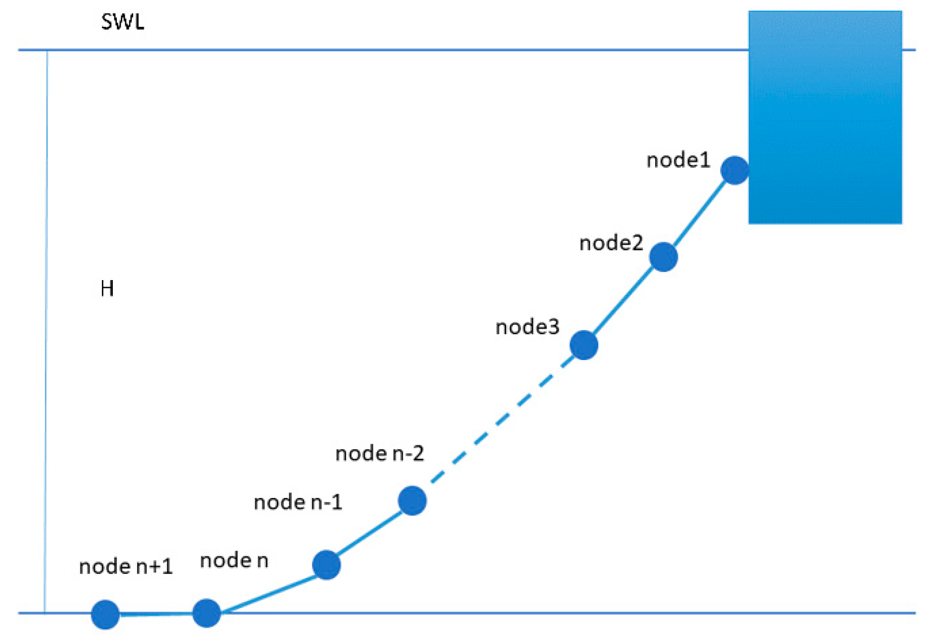
Figure 3 shows a sketch of a single mooring line. The mass of each mooring line element is lumped at both ends of the element [37].

$${\mathrm{W}}_{\mathrm{i}}=\frac{1}{2}({\mathrm{W}}_{\mathrm{i}+\frac{1}{2}}+{\mathrm{W}}_{\mathrm{i}-\frac{1}{2}}){\mathrm{n}}_{\mathrm{z}}$$

(6)

The lumped mass (mode) is connected by a massless spring and damper system. In numerical simulations, each node’s space position is determined by a space vector $r$ [37]:

$$r=\left\{\begin{array}{c}{\mathrm{x}}_{\mathrm{i}}\\ {\mathrm{y}}_{\mathrm{i}}\\ {\mathrm{z}}_{\mathrm{i}}\end{array}\right\}$$

(7)

The forces on the mooring line were evaluated by Morison’s equation [28]. The drag and inertial forces on a session length dz are

$$dF=\frac{1}{2}\rho C_{D}D{U}^{2}dz+\frac{1}{4}\rho C_M\pi D^2\frac{\partial U}{\partial t}dz$$

(8)

2.2. Correlation Analysis

Before feeding data into deep neural networks, a correlation analysis was carried out to investigate linear relationships between the most loaded line tension and the other DOFs. In general, if two features of $P$ and $Q$ are measured on $N$ individuals to the database of $\left(P_1, Q_1\right)$~$\left(P_i, Q_i\right)$~$\left(P_N, Q_N\right)$, the Pearson product-moment correlation coefficients $\mathrm{R}$ can be expressed as

$$\overline{P}=\frac{1}{N}{\displaystyle \sum }_{i=1}^N{P}_i$$

(9)

$$\overline{Q}=\frac{1}{N}{\displaystyle \sum }_{i=1}^N{Q}_i$$

(10)

$$R=\frac{{{\displaystyle \sum }}_{i=1}^N\left\{\left(P_i-\overline{P}\right)\left(Q_i-\overline{Q}\right)\right\}}{\sqrt{{{\displaystyle \sum }}_{i=1}^N{\left(P_i-\overline{P}\right)}^2}\sqrt{{{\displaystyle \sum }}_{i=1}^N{\left(Q_i-\overline{Q}\right)}^2}}$$

(11)

The Pearson product-moment correlation coefficients are widely used to identify the linear relationship between any two parameters or variables. Theoriticaly, it provides a value between +1 and −1, where +1 represents a fully positive linear correlation, 0 indicates no linear correlation and −1 characterises a fully negative linear correlation.

2.3. Deep Learning Modelling

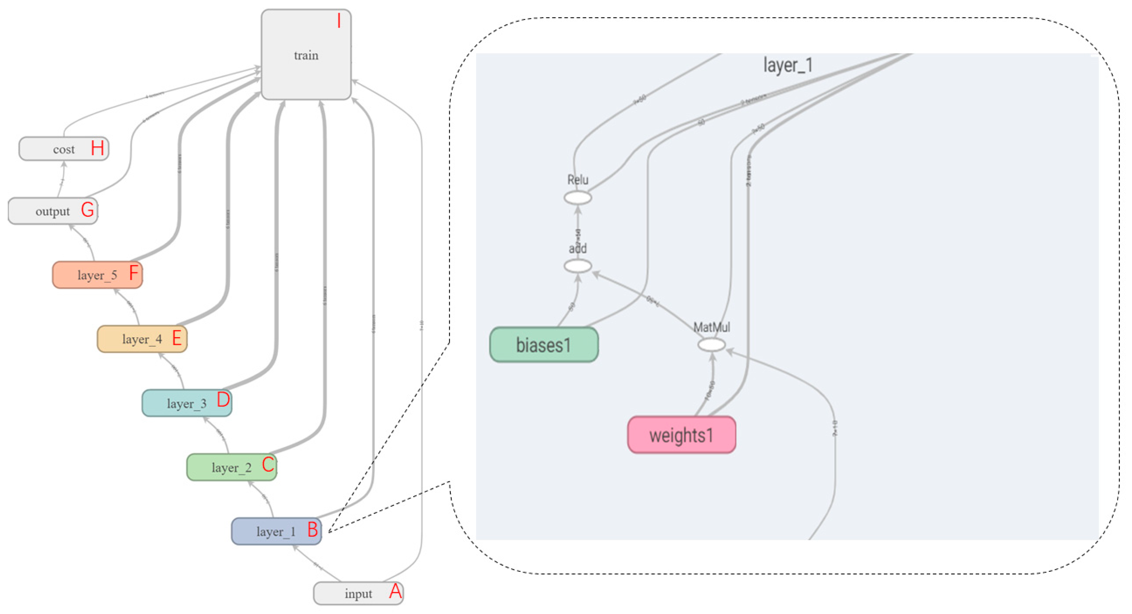
In this investigation, Keras and TensorFlow were used to develop a deep learning neural network, where input tensors were passed into a deep learning configuration and then output as another tensor (see Figure 4). In this study, different deep learning configurations were manually evaluated based on their comparative performances by trial and error. During testing and validation, the best-performing network was identified as a stacked sequential model with five layers, enclosing 50 neurons in the first and the fifth layers (see Figure 4B,F) and 100 neurons in the second, the third and the fourth layers (see Figure 4C–E). As a result, a feedforward deep learning neural network with five layers was identified to create the association between used features (see Figure 4A) and outputs (see Figure 4G). The built deep learning neural network was trained by displaying selected features (platform motions, blade deflections and tower base deflections) and desired outputs (most loaded mooring line fairlead tension). Details about the inputs in the case studies are displayed in Section 4. A scaler (Min–Max) was used to scale training, testing and validation datasets into the range between 0 and 1 after tensors flowing into different layers of the deep learning model. The expression of the scaler could be expressed as

$$F_{scaled}=\frac{f_i-\min \left(f\right)}{\max \left(f\right)-\min \left(f\right)}$$

(12)

Because all layers shared identical interior structures, only layer 1 was further expanded (see Figure 4B) to visualize the components inside layers. Each layer in the deep learning configuration contained three major components:

▪

Using Xavier’s weights initialization method [38], the present neuron and previous neurons were determined by a weight $v_{ij}$ (see Figure 4B);

▪

In the deep learning configuration, each neuron was also determined by a bias ($b_j$), for which the defaults initial bias was set as zero;

▪

The outputs of the layer were controlled by an activation function ($ReLU\left(H{N}_i\right)$), using the non-linear activation functions of Rectified Linear Unit (ReLU) (see Figure 4B).

Consequently, the following expressions are implemented in each deep learning layer:

$$H{N}_i={\displaystyle \sum }_{j=1}^m{f}_i{v}_{ij}+b_j$$

(13)

$$h=ReLU\left(H{N}_i\right)=\max \left(0, H{N}_i\right)$$

(14)

The classic train–test–validation workflow was followed while building the deep learning model. Initially, the deep learning neural network was trained (see Figure 4I) by displaying both input features and outputs to different layers. After that, based on the trained deep neural networks, testing and validation datasets were fed into the networks to carry out forecasting. The deep learning configuration was fully defined as a computational graph, in which each layer of the neural network was linked so that data flooded from the first layer through to the last layer. The inputs were randomly alienated into three groups—training group with 2.38 × 10⁵ data units (60%), testing group with 7.92 × 10⁴ data units (20%) and validation group with 7.92 × 10⁴ data units (20%). In the designed deep learning model, mean square error (MSE) was used as the cost function to measure how far predictions deviated from simulation results (see Figure 4H), which can be stated as

$$MSE=\frac{1}{p}{\displaystyle \sum }_{i=1}^p{\left[\frac{{(M_{prediction})}_i-{(M_{simulation})}_i}{{(M_{simulation})}_i}\right]}^2$$

(15)

for testing and validation data (see Figure 5).

3. Wind Turbine Properties

3.1. Structure Specifications

In this study, the target wind turbine is the DeepWind semisubmersible-type FOWT (see Figure 2) [39]. For this turbine, the rated power was 5 MW. Major properties, including rotor blade, nacelle and tower, were identical to the NREL 5MW baseline wind turbine. The floating structure was a semisubmersible type with one main column and three offset columns. The connection between these columns included several small-scale members. Total platform mass, including ballast, was 1.3473E+7 kg, and the draft of the platform was 20 m. Further specifications of the platform are given in [39].

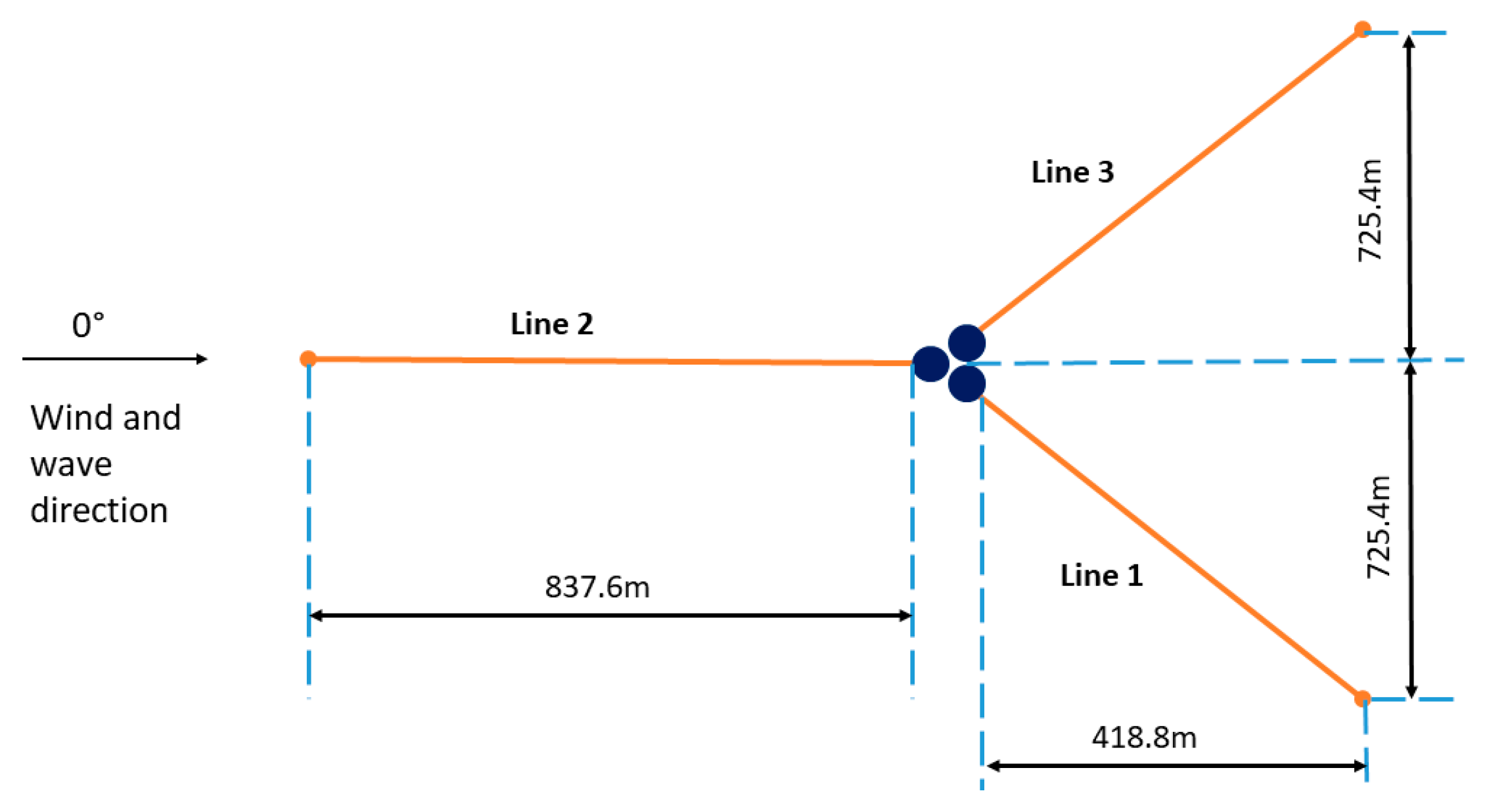
Regarding the mooring system, a spread mooring with three catenary chains was selected. Each chain had a degree of 120° between adjacent chains (see Figure 6). The total mooring chain length was 825.5 m, and the mass per unit length in water was 108.63 kg/m. The top end of the mooring line was always submerged in water, with the fairlead position located at a depth of 14 m below the SWL. Specifications of the platform and mooring lines can be found in [39].

3.2. Direct Drive Wind Turbine

3.2.1. Control methodology

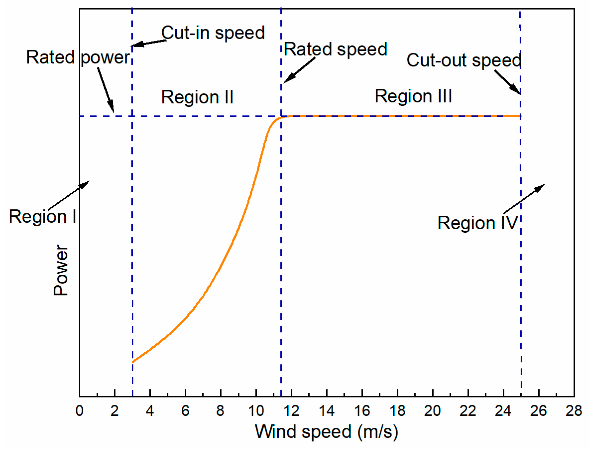
The baseline control method was applied in this study, but with a couple of modifications to fit the direct drive and the floating wind turbine. The original baseline control was designed for a fixed wind turbine with gearbox, consisting of a generator-torque controller and a blade pitch to feather control. Further details on the five regions of the control method can be found in [40]. To adapt the collective blade pitch control to a floating wind turbine with direct drive, two modifications were made. The first modification, as described in [41], included a reduction of proportional gain and integral gain to 0.006275604 and 0.0008965149 s, respectively. As can be seen in Figure 7, in total, there were four regions of operations for the FOWT. Region 1 and 4 were related to wind speeds that were equal to below cut-in and above cut-out, respectively. Therefore, power generation in these two regions was zero. The control law in region 2 was to achieve the maximum energy extraction, while region 3 relied on blade pitch control to regulate power outputs. Meanwhile, the control law in region 3 relied on a constant generator torque of 43093.55 Nm [40]. To adapt the control method to a direct drive wind turbine, the second modification included a re-development of the collective blade pitch control for a FOWT using an identical scaling method as proposed by Slot et al. [41]. A summary of modifications regarding the blade pitch control parameters is shown in

Table 1. Blade pitch control parameter modifications [39,41].

Parameter	Gearbox Wind Turbine	Direct Drive Wind Turbine	Scaling Factor
Proportional Gain	0.006275604	0.608733588	Gearbox Ratio
Integral Gain	0.0008965149	0.0869619453	Gearbox Ratio
Generator speed at the high-speed shaft end (Rad/s)	122.9096	1.2671	Gearbox Ratio

. Other parameters were the same as the scaled parameters that were presented in [41].

3.2.2. Validation of Control Method

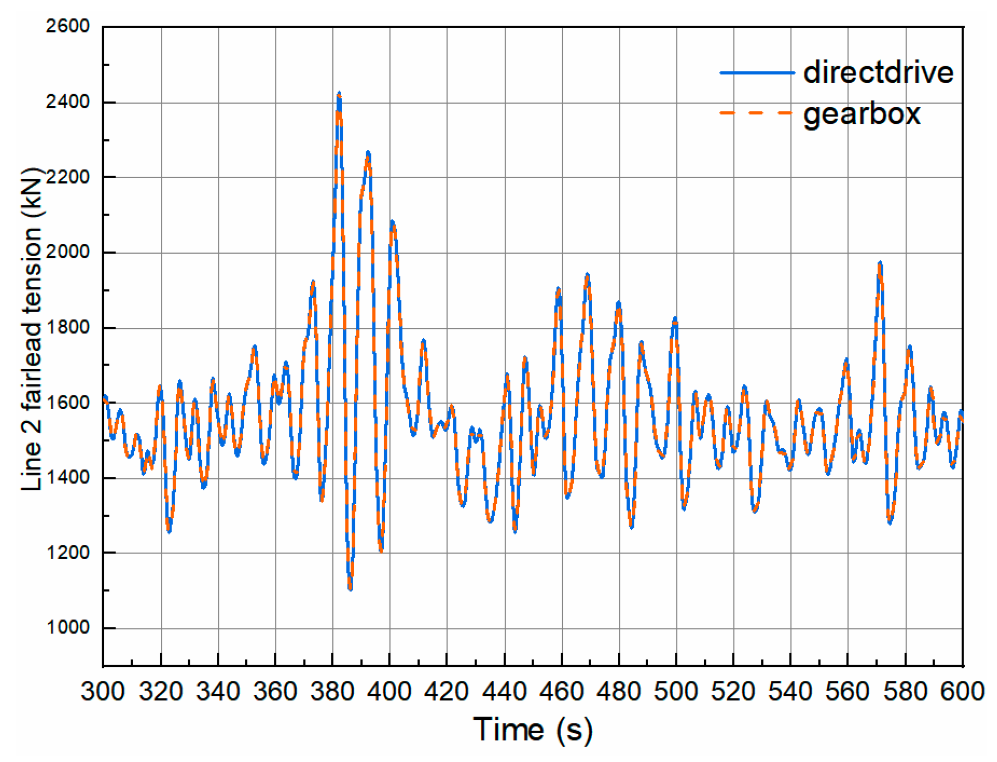
To validate the developed control method for a direct drive wind turbine, comparisons of blade pitch angles, speeds and power outputs were carried out between wind turbines with gearbox and with direct drive. The validation case studies were simulated at an average wind speed of 18 m/s under turbulent wind only conditions. As presented in Figure 8, output powers and blade pitch angles showed excellent agreement between wind turbines with and without gearbox, which further proved the accuracy of the current control method. Similar to the conclusion shown by Slot et al. [41], comparing with the case of gearbox, a direct drive wind turbine tended to generate smoother rotor torque time signals (see Figure 8).

A further comparison is shown in Figure 9, focusing on the most loaded mooring line tension of the FOWT. It can be concluded that the drive train model seldom influenced mooring line tensions.

4. Case Studies and Discussion

4.1. Load Cases and Inputs for the Deep Learning Model

For parked wind turbines, the global performance and the effect from mooring line tension are identical to traditional oil and gas platforms. Therefore, case studies of this investigation have focused on wind turbine operating conditions only. A number of wind speeds were considered ranging from cut-in to cut-out scenarios. A list of case studies is shown in

Table 2. Load cases [42].

Load Case Number	Wind Speed (m/s)	HS (m)	TP (s)
1	4	1.7	11.6
2	6	1.9	11.3
3	8	2.1	11.0
4	10	2.4	10.8
5	12	2.8	10.7
6	14	3.2	10.7
7	16	3.7	10.8
8	18	4.2	10.8
9	20	4.7	11.0
10	22	5.4	11.1
11	24	6.0	11.3

.

Inputs of the designed deep learning model were generated from a time-domain AHSE model as described in Section 2.1. For the present case studies, a total number of ten inputs were selected (see

Table 3. Input features of deep learning neural networks.

Parameter		Description
Blade	TipDxb1	Blade 1 flapwise tip deflection
	TipDyb1	Blade 1 edgewise tip deflection
Tower	TTDspFA	Tower-top fore-aft deflection
	TTDspSS	Tower-top side-to-side deflection
Platform	PtfmSurge	Platform Surge Motion
	PtfmSway	Platform Sway Motion
	PtfmHeave	Platform Heave Motion
	Ptfmroll	Platform Roll Motion
	PtfmPitch	Platform Pitch Motion
	PtfmYaw	Platform Yaw Motion

), which were the 6-DOF platform motion responses, the two tip deflections of blades and the two tower top deflections.

4.2. Load Cases and Inputs for the Deep Learning Model

Before processing the results from the AHSE model into the deep learning neural network, it is necessary to pre-process and analyse the data properties. To this end, a series of histograms of the most loaded mooring line tension was generated, based on the AHSE results. All the distributions satisfied the normal distribution. More specifically, the majority of counts were located in the middle of the distribution graph, while the tails had the minimum number of counts. Figure 10 shows an example of the histogram of mooring line tension of load case 11 (see

Table 4. Comparison of statistical data (slack mooring line).

Model	Mean (kN)	Min (kN)	Max (kN)
Flexible	1498.02	1140.00	2097.00
Rigid	1496.93	1140.00	2092.00
Difference (%)	0.72	0.00	2.38

) for slack mooring system.

Using the heatmap, the correlation between the input features and the most loaded mooring line tension is put forward through a calculation of Pearson product-moment correlation coefficients (Figure 11). The individual coefficients contained in a matrix are represented by colours from red to blue. As presented in Figure 11, mooring line tension was strongly correlated with the platform surge motion, followed by the pitch and the tower top fore-aft deflection. On the other hand, compared with the surge or the tower top fore-aft deflection, the platform heave motion had a correlation coefficient of 0.26, indicating a less significant relationship with the mooring line tension. However, correlation analysis is designed for analysing linear relationships only. The inherent mechanism in determining mooring line tension may not necessarily follow a linear relationship. To this end, a machine learning approach capable of dealing with nonlinear relationships is used and presented in Section 4.3.

4.3. Level of Significance

The level of significance of features in simulating outputs was examined. Owing to the aim of this investigation to identify the important input features and simulate mooring line tensions, the final MSEs in the deep learning model were used to identify the features. For this reason, in the deep learning model, only one feature was represented by its mean value in the validation loop at each trial. Since just one feature was altered at one time, this analysis was repeated on all the ten inputs one by one, as shown in Figure 12. Variations of MSEs along validation loops under each feature change are presented in Figure 12. Basically, all the inputs influenced the accuracy of the predicted output of the designed deep learning configuration, as the column ‘original’ is located at the very left of Figure 12. The platform surge had the largest final MSE, showing that it played a dominant role in the accuracy of the designed neural networks. Furthermore, it has a much larger amplitude of the final MSE than the others, unlike the blade and the tower bending effects (such as TipDyb1: blade 1 out-of-plane tip deflection, TTDspSS: tower top side-to-side deflection, and TTDspFA: tower top fore-aft deflection).

4.4. Discussions

4.4.1. Effects of Tower and Blade Flexibility—Slack Mooring Line

Based on the result from Section 4.3, a comparison between two case studies (1) enabling all the blade and tower bending modes and (2) rigid body assumptions for the tower and blades were carried out using the time-domain AHSE model, as shown in Figure 13. The average wind speed was 24 m/s. The total simulation time was 15 min, with a total number of five realisations. Mooring line top tension results from one of the realisations were shown in Figure 13. Results based on the two modelling approaches, with or without the consideration of tower and blade elasticities, were in excellent agreement with each other. For comparison, statistical data based on the results from Figure 13 are described in Table 4, which showed identical conclusions in Figure 13. In other words, the most loaded line tension can be evaluated accurately with a model of rigid tower and blade.

4.4.2. Effects of Mooring Configuration—Taut Mooring Line

Slack and taut mooring configurations are the most widely applied mooring types. Section 4.4.1 discussed the effects from tower and blade elasticities for a slack mooring line configuration. In this section, a further case study was investigated with a focus on the taut mooring system configuration. For consistency in this paper, both taut and slack mooring configurations followed a similar static load–offset graph (see Figure 14), in terms of the horizontal restoring force. The load–offset graph (see Figure 14) was generated based on the slack mooring configuration, as shown in Table 2, using OrcaFlex [43] for a number of horizontal offsets ranging from 0 to 16 m. Based on the load–offset graph, taut mooring line configurations were determined through the mooring materials provided by [44], while at the same time having the identical load–offset behaviour as described in Figure 14. Detailed properties for the taut mooring line, the corresponding fairlead and the anchor positions are listed in

Table 5. Taut mooring line properties [43,44].

Parameter	Value
Rope/Wire Properties nominal diam	0.2 m
Weight in air	0.313 kN/m (0.032 te/m)
Displacement	0.234 kN/m (0.024 te/m)
Weight in water	0.079 kN/m (0.0081 te/m)
Diam/Wt ratio	2.166 m/(kN/m) (21.245 m/(te/m))
EA	43.6E3 kN
Added mass	1.0
Line length	245 m

and

Table 6. Mooring line position.

Line No		Position
		X (m)	Y (m)	Z (m)
Line1	Fairlead	−40.868	0	−14
	Anchor	−200	0	0
Line2	Fairlead	20.434	35.3917	−14
	Anchor	100	173.2	0
Line3	Fairlead	20.434	−35.3917	−14
	Anchor	100	−173.2	0

.

Using the identical deep learning configuration mentioned in Section 2.2 and Section 2.3, a ranking of the contributions of all the inputs on the mooring line top tension is displayed in Figure 15. Unlike slack moorings, the contributions from inputs in taut mooring lines are purely dominated by surge motion.

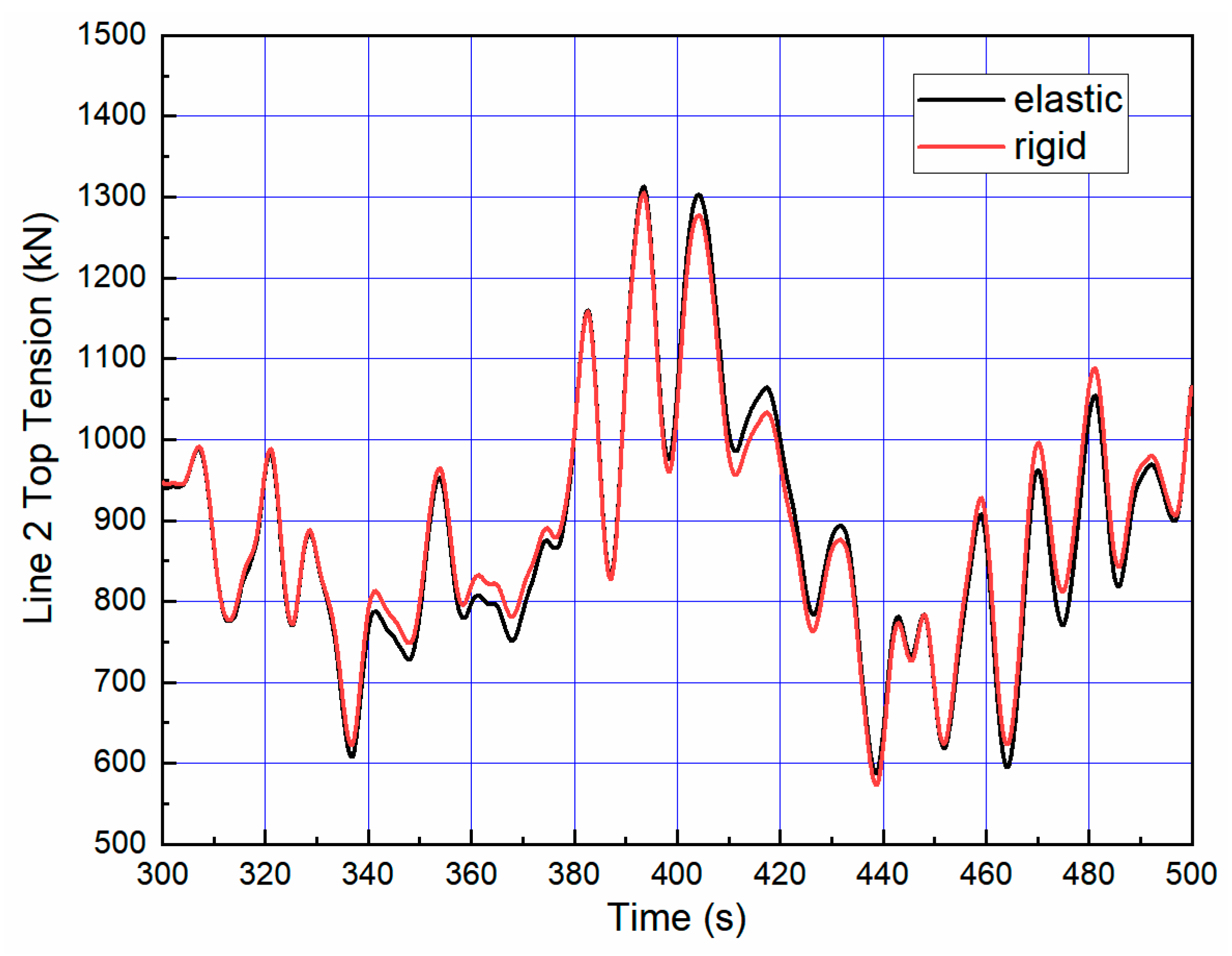
Similarly, a further verification was performed using the time-domain AHSE model with rigid tower and blade considered. The average wind speed was 24 m/s, and the corresponding wave parameters for the random wave simulations were 6 m significant wave height and 11.3 peak period (Table 4). Figure 16 shows a comparison of mooring line 2 top tensions under rigid and elastic models for the blade and tower.

Compared with slack mooring lines, a more obvious difference was identified when it came to taut mooring lines (see Figure 13; Figure 16). However, the differences remained within 5% (see

Table 7. Comparison of statistical data (taut mooring line, average wind speed of 24 m/s).

Model	Mean (N)	Minimum (N)	Maximum (N)
flexible	860,955.51173	313,500	1,313,000
rigid	863,705.90408	328,400	1,305,000
Difference (%)	0.3	4.8	0.6

).

5. Conclusions

A novel methodology has been developed to quantify the driven forces on FOWT mooring line tension. The input features of deep learning neural networks were extracted from a nonlinear time-domain AHSE model under various environmental conditions. A deep learning model was trained, tested and validated to investigate the level of significance of different input features on the mooring line tension. In the proposed deep learning model, a total number of ten features was used as the inputs, while the most loaded mooring line tension was chosen as the output variable. The advantage of the proposed model lies in its accounting for different environmental conditions automatically.

Key conclusions of this paper are summarised as follows:

• A deep learning model has been successfully built to rank the level of contributions to predicting the most loaded mooring line tension. Its accuracy has been validated against the nonlinear time-domain method.
• A numerical model has been developed on blade pitch control for a direct drive train configuration with FOWT, while its accuracy has been validated against gearbox wind turbine. Good agreement has been achieved in terms of blade pitch angles for above-rated wind conditions because of the perfect match of shaft speed.
• For the slack mooring configuration, the most loaded mooring line tension is mainly dominated by the platform surge motion, while the pitch and the heave have almost equal contributions to the tension, but not as important as surge. For taut mooring lines, the most loaded line tension is purely determined by surge, while other parameters are less significant.
• Compared with surge motion, blade and tower elasticities are insignificant for predicting FOWT most loaded mooring line tension, regardless of the mooring system types (slack or taut).

References

1. Wang, X.; Zeng, X.; Yang, X.; Li, J. Feasibility study of offshore wind turbines with hybrid monopile foundation based on centrifuge modeling. Appl. Energy 2018, 209, 127–139. [Google Scholar] [CrossRef]
2. Chen, J.; Wang, F.; Stelson, K.A. A mathematical approach to minimizing the cost of energy for large utility wind turbines. Appl. Energy 2018, 228, 1413–1422. [Google Scholar] [CrossRef]
3. Waters, L.; Spry, W. Energy Trends December 2018, Section 6: Renewables; Department for Business, Energy & Industrial Strategy: London, UK, 2018.
4. Liu, X.; Lu, C.; Li, G.; Godbole, A.; Chen, Y. Effects of aerodynamic damping on the tower load of offshore horizontal axis wind turbines. Appl. Energy 2017, 204, 1101–1114. [Google Scholar] [CrossRef] [Green Version]
5. Gao, X.; Wang, T.; Li, B.; Sun, H.; Yang, H.; Han, Z.; Wang, Y.; Zhao, F. Investigation of wind turbine performance coupling wake and topography effects based on LiDAR measurements and SCADA data. Appl. Energy 2019, 255, 113816. [Google Scholar] [CrossRef]
6. Dai, J.; Yang, X.; Hu, W.; Wen, L.; Tan, Y. Effect investigation of yaw on wind turbine performance based on SCADA data. Energy 2018, 149, 684–696. [Google Scholar] [CrossRef]
7. Le, C.; Li, Y.; Ding, H. Study on the coupled dynamic responses of a submerged floating wind turbine under different mooring conditions. Energies 2019, 12, 418. [Google Scholar] [CrossRef] [Green Version]
8. Liu, Z.; Zhou, Q.; Tu, Y.; Wang, W.; Hua, X. Proposal of a Novel Semi-Submersible Floating Wind Turbine Platform Composed of Inclined Columns and Multi-Segmented Mooring Lines. Energies 2019, 12, 1809. [Google Scholar] [CrossRef] [Green Version]
9. Luo, T.; Tian, D.; Wang, R.; Liao, C. Stochastic dynamic response analysis of a 10 MW tension leg platform floating horizontal axis wind turbine. Energies 2018, 11, 3341. [Google Scholar] [CrossRef] [Green Version]
10. Cheng, Z.; Rui, T.; Chen, M.; Wang, K. Power performance and dynamic responses of a combined fl oating vertical axis wind turbine and wave energy converter concept. Energy 2019, 171, 190–204. [Google Scholar] [CrossRef]
11. Kokubun, K.; Ishida, S.; Nimura, T.; Chujo, T.; Yoshida, S.; Utsunomiya, T. Model Experiment Of A Spar Type Offshore Wind Turbine In Storm Condition. In Proceedings of the ASME 2012 31st International Conference on Ocean, Offshore and Arctic Engineering, Rio de Janeiro, Brazil, 1–6 July 2012; ASME: Rio de Janeiro, Brazil, 2012; pp. 569–575. [Google Scholar]
12. Li, Y.; Zhu, Q.; Liu, L.; Tang, Y. Transient response of a SPAR-type floating offshore wind turbine with fractured mooring lines. Renew. Energy 2018, 122, 576–588. [Google Scholar] [CrossRef]
13. Seebai, T.; Sundaravadivelu, R. Effect of Damaged Mooring Line on Response of Spar with Wind Turbine. J. Inst. Eng. (India) Ser. A 2012, 93, 9–14. [Google Scholar] [CrossRef]
14. Bae, Y.H.; Kim, M.H.; Kim, H.C. Performance changes of a floating offshore wind turbine with broken mooring line. Renew. Energy 2017, 101, 364–375. [Google Scholar] [CrossRef]
15. Ma, G.; Zhong, L.; Ma, Q.; Zhu, Y.; Wang, H. Dynamic Analysis of Mooring Break for a Semi-Submersible Floating Offshore Wind Turbine. In Proceedings of the Twenty-ninth (2019) International Ocean and Polar Engineering Conference, Honolulu, HI, USA, 16–21 June 2019; The International Society of Offshore and Polar Engineers (ISOPE): Mountain View, CA, USA, 2019; pp. 356–362. [Google Scholar]
16. Li, Y.; Le, C.; Ding, H.; Zhang, P. Dynamic Response for a Submerged Floating O ff shore Wind Turbine with Di ff erent Mooring Configurations. J. Mar. Sci. Eng. 2019, 7. [Google Scholar]
17. Seven Mechanisms That Contribute to Mooring Line Failure. Available online: https://intermoor.com/technical-articles/six-mechanisms-that-can-contribute-to-mooring-line-failure/ (accessed on 7 April 2020).
18. Wang, X.; Zeng, X.; Yang, X.; Li, J. Seismic response of offshore wind turbine with hybrid monopile foundation based on centrifuge modelling. Appl. Energy 2019, 235, 1335–1350. [Google Scholar] [CrossRef]
19. Doubrawa, P.; Churchfield, M.J.; Godvik, M.; Sirnivas, S. Load response of a floating wind turbine to turbulent atmospheric flow. Appl. Energy 2019, 242, 1588–1599. [Google Scholar] [CrossRef]
20. Gentils, T.; Wang, L.; Kolios, A. Integrated structural optimisation of offshore wind turbine support structures based on finite element analysis and genetic algorithm. Appl. Energy 2017, 199, 187–204. [Google Scholar] [CrossRef] [Green Version]
21. Leble, V.; Barakos, G.N. A Coupled Floating Offshore Wind Turbine Analysis with High-fidelity Methods. Energy Procedia 2016, 94, 523–530. [Google Scholar] [CrossRef] [Green Version]
22. Chehouri, A.; Younes, R.; Ilinca, A.; Perron, J. Review of performance optimization techniques applied to wind turbines. Appl. Energy 2015, 142, 361–388. [Google Scholar] [CrossRef]
23. Jonkman, B.J.; Jonkman, J.M. FAST v8.16.00a-bjj User’s Guide; National Renewable Energy Laboratory: Golden, CO, USA, 2016.
24. Glauert, H. Airplane Propellers. In Aerodynamic Theory; Springer: Berlin/Heidelberg, Germany, 1935. [Google Scholar]
25. Moriarty, P.J.; Hansen, A.C. AeroDyn Theory Manual; National Renewable Energy Laboratory: Golden, CO, USA, 2005.
26. Ingram, G. Wind Turbine Blade Analysis Using the Blade Element Momentum Method; Durham University: Durham, UK, 2011. [Google Scholar]
27. WAMIT 6.2 User Manual. Available online: http://www.wamit.com/ (accessed on 7 April 2020).
28. Morison, J.R.; Johnson, J.W.; Schaaf, S.A. The Force Exerted by Surface Waves on Piles. J. Pet. Technol. 1950. [Google Scholar] [CrossRef]
29. Zandt, T. Van FAST User’s Guide. Acta Psychiatr. Scand. 2007, 123, 407–408. [Google Scholar]
30. Kurian, V.J.; Yassir, M.A.; Harahap, I.S. Nonlinear coupled dynamic response of a semi-submersible platform. In Proceedings of the International Offshore and Polar Engineering Conference, Beijing, China, 20–25 June 2010; Volume 3, pp. 492–499. [Google Scholar]
31. Faltinsen, O.M. Sea Loads on Ships and Offshore Structures; Cambridge University Press: Cambridge, MA, USA, 1993. [Google Scholar]
32. Vu, M.T.; Van, M.; Bui, D.H.P.; Do, Q.T.; Huynh, T.T.; Lee, S.D.; Choi, H.S. Study on dynamic behavior of unmanned surface vehicle-linked unmanned underwater vehicle system for underwater exploration. Sensors (Switz.) 2020, 20, 1329. [Google Scholar] [CrossRef] [PubMed] [Green Version]
33. The Vu, M.; Choi, H.S.; Kang, J.; Ji, D.H.; Jeong, S.K. A study on hovering motion of the underwater vehicle with umbilical cable. Ocean Eng. 2017, 135, 137–157. [Google Scholar] [CrossRef]
34. Low, Y.M.; Langley, R.S. A hybrid time/frequency domain approach for efficient coupled analysis of vessel/mooring/riser dynamics. Ocean Eng. 2008, 35, 433–446. [Google Scholar] [CrossRef]
35. Goodman, T.R.; Breslin, J.P. Statics and Dynamics of Anchoring Cables in Waves. J. Hydronautics 1976, 10, 113–120. [Google Scholar] [CrossRef]
36. Low, Y.M.; Langley, R.S. Time and frequency domain coupled analysis of deepwater floating production systems. Appl. Ocean Res. 2006, 28, 371–385. [Google Scholar] [CrossRef]
37. Hall, M.; Goupee, A. Validation of a lumped-mass mooring line model with DeepCwind semisubmersible model test data. Ocean Eng. 2015, 104, 590–603. [Google Scholar] [CrossRef] [Green Version]
38. Dewa, C.K. Afiahayati Suitable CNN Weight Initialization and Activation Function for Javanese Vowels Classification. Procedia Comput. Sci. 2018, 144, 124–132. [Google Scholar] [CrossRef]
39. Robertson, A.; Jonkman, J.; Masciola, M.; Song, H. Definition of the Semisubmersible Floating System for Phase II of OC4; National Renewable Energy Laboratory: Golden, CO, USA, 2014.
40. Jonkman, J.; Butterfield, S.; Musial, W.; Scott, G. Definition of a 5-MW Reference Wind Turbine for Offshore System Development; National Renewable Energy Laboratory: Golden, CO, USA, 2009.
41. Slot, R.M.M.; Svenningsen, L. Consistent direct-drive version of the NREL 5MW turbine. In Proceedings of the WindEurope, Hamburg, Germany, 25–28 September 2018. [Google Scholar]
42. Li, Q.; Michailides, C.; Gao, Z.; Moan, T. A comparative study of different methods for predicting the long-term extreme structural responses of the combined wind and wave energy concept semisubmersible wind energy and flap-type wave energy converter. Proc. Inst. Mech. Eng. Part M J. Eng. Marit. Environ. 2018, 232, 85–96. [Google Scholar] [CrossRef]
43. OrcaFlex. Available online: https://www.orcina.com/orcaflex/ (accessed on 7 April 2020).
44. Azcon, J.; Vittori, F.; Savenije, F.; Kapogiannis, G.; Karvelas, X.; Manolas, D.; Voutsinas, S.; Amann, F.; Ricardo, F.-G.; Lemmer, F. Design Solutions for 10MW Floating Offshore Wind Turbines; INNWIND: Roskilde, Denmark, 2017. [Google Scholar]
Figure 1. Configuration of methodologies.
Energies 13 02264 g001
Figure 2. Definition of floating body 6-DOF (Degree of Freedom) coordinate.
Energies 13 02264 g002
Figure 3. Lumped-mass and spring model.
Energies 13 02264 g003
Figure 4. Designed deep learning configuration.
Energies 13 02264 g004
Figure 5. Variations of training, testing and validation mean square errors (MSEs) along 200 epochs in the designed deep learning configuration.
Energies 13 02264 g005
Figure 6. Wind/wave directions and mooring line orientations.
Energies 13 02264 g006
Figure 7. Regions of operations.
Energies 13 02264 g007
Figure 8. Validations of the control method on a direct drive floating offshore wind turbine (FOWT).
Energies 13 02264 g008
Figure 9. Most loaded line (line 2) fairlead tension (time history).
Energies 13 02264 g009
Figure 10. Histogram of most loaded mooring line tension of load case 11 (slack mooring).
Energies 13 02264 g010
Figure 11. Heat map (slack mooring line).
Energies 13 02264 g011
Figure 12. Variations of final MSEs in different sensitivity analysis scenarios.
Energies 13 02264 g012
Figure 13. Comparison of line 2 top tension (rigid and flexible tower/blades).
Energies 13 02264 g013
Figure 14. Load offset graph in the X direction.
Energies 13 02264 g014
Figure 15. Level of significance (taut).
Energies 13 02264 g015
Figure 16. Comparison of mooring line tensions between elastic and rigid models for the tower and blades (taut mooring).
Energies 13 02264 g016