Evaluating Building Energy Code Compliance and Savings Potential through Large-Scale Simulation with Models Inferred by Field Data ^†

Abstract

Building energy code compliance is the crucial link between the actual energy savings and the efficiency prescribed in energy codes. A research project aiming to identify opportunities to reduce energy consumption in new single-family residential construction by increasing compliance with the building energy code was conducted in several states of the United States. The study was comprised of three phases: (1) a baseline study to document typical practice and identify opportunities for improvement based on empirical data gathered from the field; (2) an education and training phase targeting the opportunities identified; and (3) a post-study to assess whether a reduction in average state-wide energy use could be achieved following the education and training phase. We proposed a novel methodology based on large-scale building energy simulation inferred by limited field data to assess the performance of a large population of homes. This paper presents the methodology, findings, and results of this study. The state-wide average energy consumption decreased at Phase III from Phase I for five of the seven states involved in the analysis. The measure-level savings potential analysis shows an overall reduction. Overall, the training and education phase plays a recognizable role in improving compliance with building energy codes.

1. Introduction

In the United States (U.S.), building energy use was responsible for 40% of total energy consumption and 75% of total electricity consumption in 2016 [1]. As a cost-effective manner for reducing energy usage, building energy codes, which govern building construction to meet minimum energy requirements, have been implemented and regularly strengthened for new and existing buildings in many countries [2].

Building energy codes have many advantages, such as lower utility bills for consumers, improved energy resilience, health and comfort, environmental sustainability, and a lower need for energy subsidies [2,3]. Studies have shown that building energy codes have led to 6%–22% reduction of average annual energy consumption per dwellings in the residential building sector of the European Union [2,4], have the potential to curtail the energy usage and CO₂ emissions by 13%–22% by 2100 in China [5], and could dwindle building electricity use in Gujarat, India by 20% in 2050 [6]. In the U.S., building energy codes have helped saving approximately 4.2 quads of energy and more than $44 billion for customers between 1992 and 2012 [7]. Athalye et al. [8] evaluated the national impact of energy codes from 2010 to 2040 by accounting for the varying rates that states adopt the model building codes and a modest pace at which energy codes update over the years, and they estimated that building energy codes could bring $126 billion savings to consumers’ utility bills in that timeframe, which equates to a carbon pollution cutback of 841 million metric tons: an equivalent to the greenhouse gases emitted by 177 million passenger vehicles driven for one year or the carbon dioxide emissions from 245 coal power plants for one year or 89 million homes. Nowadays, it is widely accepted that building energy codes do help save energy [3,9,10,11].

Code compliance is a vital link between actual energy savings and the energy efficiency prescribed in the energy code books [12,13]. The energy savings from stringent energy codes cannot be delivered unless new buildings are constructed to completely comply with the code. Non-compliance has been noted as an issue internationally, e.g., in the United Kingdom, [14], U.S. [12], China [13,15], and many other developing countries [16]. It also seems that countries such as China with a mandatory energy efficiency code show quite high compliance [15], and the effectiveness of the building energy efficiency standards (BEES) of China was confirmed through field study and analysis with a data-driven approach [17]. In the U.S., state legislatures, local government, utility companies, and energy efficiency organizations are interested in knowing the status quo of code compliance and the energy-savings potential in their jurisdictions [12]. Obsolete building codes hurt the international competition of the U.S. construction industry [3]. Knowing the status quo allows the state to identify common causes of non-compliance and assess the energy and economic impacts of updating to a more stringent code [18]. Identifying key technology trends and quantifying the value of increased compliance are often required by state regulatory agencies (e.g., utility commissions) as a prerequisite to assigning value and attribution for programs contributing to state energy efficiency goals [18]. Utilities also rely on energy code compliance for resource planning and the payback of investments [19], and they are credited with energy savings from their code compliance assistance efforts [13]. Improving code compliance could have tremendous economic impact. Research estimates that the national savings from ensuring just one year’s worth of new residential and commercial construction in the U.S. to complete compliance to the building energy code is 2.8–8.5 trillion Btu annually, or $63–$189 million in energy cost savings annually, which equates to lifetime savings of up to $37 billion for just five years of construction. [12]. A study conducted by the Institute for Market Transformation (IMT) indicated that every dollar spent on code compliance and enforcement efforts leads to a six-fold return in energy savings [20].

Historically, most building energy code compliance studies do not directly estimate energy savings due to compliance rate methods, relying on some form of prescriptive checklist being the most commonly used approach [12,21]. A compliance rate captures the fraction of buildings that meet all the prescribed code requirements. Most compliance evaluations stop at providing merely a compliance rate; however, simply knowing the compliance rate makes it difficult to estimate the potential energy savings impact of improved compliance [21,22]. Additional analysis is needed to convert the raw or aggregate compliance scores resulting from a checklist or pass–fail approach into energy metrics [12]. Prescriptive checklists were developed with the possible weighting of code items to account for varying energy impacts [23,24]. In addition, code compliance evaluation requires multiple site visits to complete a survey; based on the given stage of the construction process, a measurement can be recorded. These surveys are expensive, as it is difficult to collect enough data points to perform engineering calculations or computer simulations that would provide statistically representative code compliance rates at the state level.

As more builders follow the performance pathway to meet building energy code requirements, building energy performance metrics and building energy simulation models serve a greater role in conducting code compliance evaluation [25,26]. Building simulation has been widely used to support building energy-efficiency study for a variety of research and practical purposes. Compared to in situ building experiments, building energy simulation provides a numerical experiment with a relatively fast, low-cost, and controllable environment to investigate the impact of design choices and technologies on an overall building’s energy performance. There are many sophisticated building energy modeling tools that apply physics-based principles to simulate detailed building energy patterns. EnergyPlus [27] is one that has been used widely for the building energy codes development in the U.S. and was thus chosen for the evaluation of code compliance in this study.

There are several challenges of using building simulation to evaluate the energy impacts of code compliance. One of the primary challenges is having enough data inputs to inform the building energy model. When building energy simulation is used to compare individual building design options and technologies or evaluate retrofit measures, model inputs can be derived from building design blueprints, building permits, or from actual observations of individual buildings under retrofit. Prototypical building models are generally used to support energy code development or evaluate energy efficiency measures for a population of buildings [28,29,30]. The general energy characteristics of the prototypical buildings are known as well as the operations and control schemes [31,32]. However, these assumptions are not necessarily valid to develop a building simulation tool based off code compliance measurements taken from actual buildings.

The evaluation of code compliance requires in-field data collection to compare results against minimum code requirements. The average completion time of a single-family home is around several months, and the entire building construction process is complex. These make it very difficult to know whether a home complies with the energy code in its entirety, as not all energy-efficiency measures are in place or visible at any given point during the home construction process. For example, when homes are visited during earlier stages of construction, key features affecting energy performance (e.g., walls with insulation) may not be in place yet. However, these items may also not be observable, because they might be already covered if the homes are visited during later stages. Therefore, to gather all the data required in the sampling plan, field teams needed to visit homes in various stages of the construction process [24]. Multiple site visits during different construction phases not only increases the survey cost, but also introduces biases on the data collection due to the awareness of the builder of the upcoming visits. The builder’s practice may be altered by knowing there are follow-up compliance assessments in the future. To account for these potential biases, field visits are conducted on a small sample of buildings where code items are recorded from a variety of different homes. As such, no home provides a complete representation of its compliance.

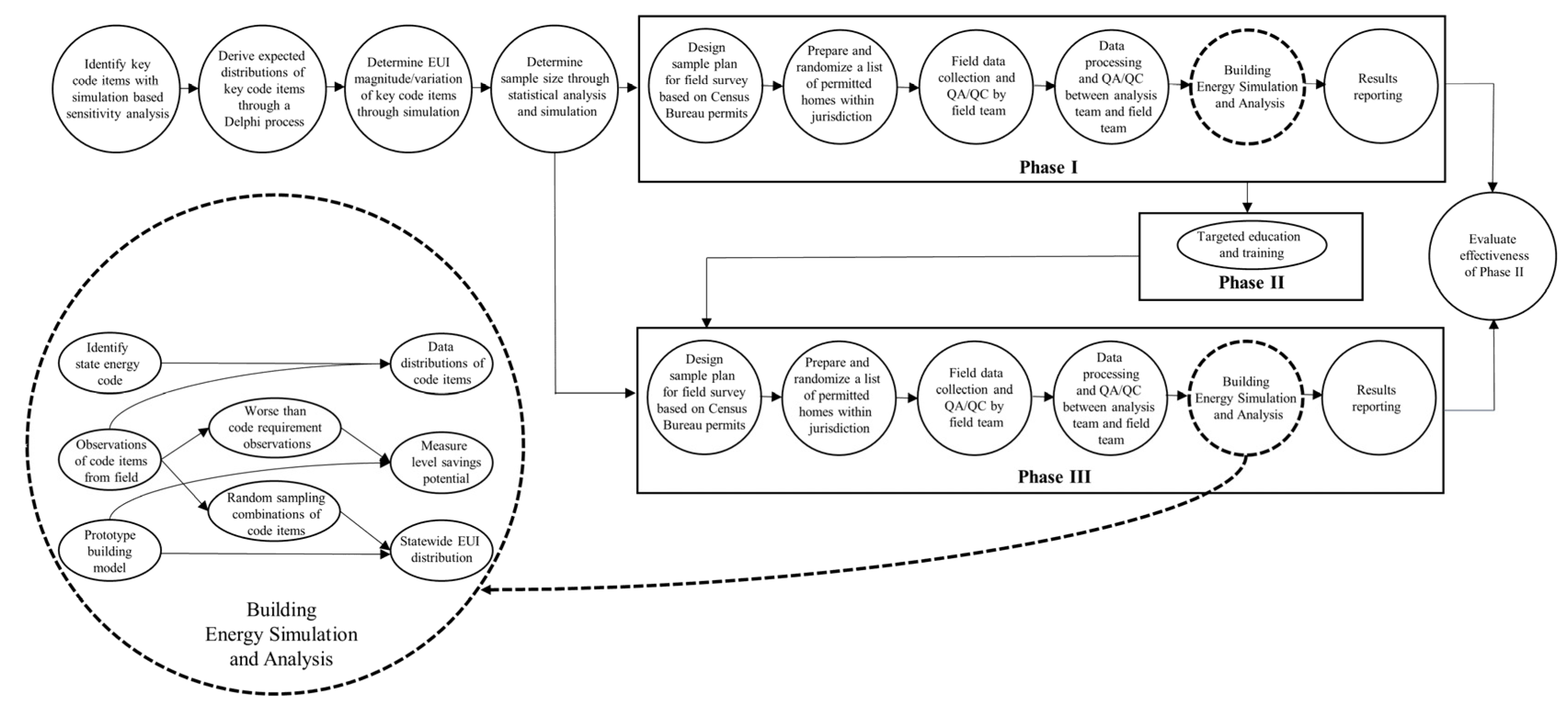
This shortage of complete data for individual homes introduces an analytical challenge, because building energy simulation tools require a complete set of inputs to generate reliable results [24]. Since comprehensive field surveys for the energy simulation of individual buildings becomes impractical for a code compliance evaluation at the scale of an entire state, this study leverages a novel modeling framework to limited field data collection with large-scale simulation. The framework consists of all aspects of conducting a residential energy code field study in single-family homes, including sampling homes under construction for field visit, data collection during a site survey, and the subsequent building energy simulation and analysis. The research questions we are trying to address include determining the status quo of code compliance in the new single-family homes in a state in terms of building energy consumption, the energy impact of non-compliance with energy codes, and whether targeted education and training could reduce the non-compliance and its impact.

The entire study includes three phases. Phase I establishes a baseline to evaluate the status quo of energy use in typical new construction residential homes in the state and identify specific code items that are not complied with, and therefore can be targeted to achieve better energy savings. Once specific code measures are identified, specific education, training, and outreach activities can be developed for Phase II. These multi-year activities are offered to builders to improve compliance rates and installation practices. Phase III is the final stage of the field studies, where follow-up field data is conducted, following the same survey methodology from Phase I. This paper focuses on the complete data analysis of Phase III, the comparison of analysis results between Phase III and Phase I, providing results on the impact of the education and training activities on code compliance and energy-savings potential.

The remainder of this paper is organized into five sections. Section 2 provides an overview of the three phases of this study and states participating in the initial pilot. Section 3 introduces the aspects of the framework that have otherwise been described and applied in Phase I [33] and part of Phase III [34] with a focus on the comparison between phases. Section 4 presents the results for seven states of the U.S. Section 5 describes the larger impact and opportunities that the code studies present. Section 6 concludes the paper and summaries the key contributions.

2. Background

Building energy codes save energy, and savings can be theoretically quantified through code-book to code-book comparison with the aid of computer simulation. However, construction is neither a simulation model nor a physical laboratory; the savings that assume perfect code compliance do not reflect reality. The commonly used checklist compliance rate approach has weaknesses because it is assumed to be a proxy for energy, but that connection was never empirically established [35]. Little research has been done to evaluate compliance in a consistent and reproducible manner, due to the complex nature of this matter [36]. To address the lack of information available on energy code impacts, the U.S. Department of Energy initiated an Energy Code Field Study to help documenting baseline practices and targeting areas for improvement as well as further quantifying related savings potential [24]. This information is intended to assist states in measuring energy code compliance and to identify areas of focus for future education and training initiatives [37].

A multi-year residential energy code field study was initiated by the United States Department of Energy (U.S. DOE) in 2015. The goal of the study was to determine whether an investment in education, training, and outreach programs targeted at improving code compliance can produce a significant, measurable change in single-family residential building energy use [35]. The study consists of (1) establishing a framework to evaluate the current status of code compliance and quantify code-related energy savings opportunities in single-family residential construction, and (2) testing whether compliance could be improved through energy code education, training, and outreach activities. Eight U.S. states, including Alabama (AL), Arkansas (AR), Georgia (GA), Kentucky (KY), Maryland (MD), North Carolina (NC), Pennsylvania (PA), and Texas (TX) participated in the pilot study by responding to the U.S. DOE Funding Opportunity Announcement (FOA), “Strategies to Increase Residential Energy Code Compliance Rates and Measure Results” [37,38].

The study includes three phases. A framework for evaluating residential building code compliance has been developed during Phase I. The framework includes plans for site surveys, protocols for data collection, and a methodology for data analysis including EnergyPlus simulation. The analysis methodology replaces the historic compliance rate approach with the use of building energy simulation [24]. Prototype building models are used for the analysis. Limited field data is collected and bootstrap sampling [39,40] is applied to generate inputs for many building models on which EnergyPlus simulation is conducted. Bootstrap is a widely used computational-intensive statistical tool based on empirical distribution, and the repeated sampling with replacement on it for improving statistical assessment of the population. It has increasing use in the energy efficiency area [41,42,43]. In the context of assessing code compliance in a state, the population is all the new homes constructed in one year. While it is not possible to survey all homes under construction, ideally one wants to draw large, non-repeated, samples from the population. However, one is generally limited to one sample with limited instances because of limited resources. Like other statistics tools, bootstrap is based on the plug-in principle, which is to substitute something unknown with an estimate [39,40]. For example, one uses sample mean as an estimate of population mean. With bootstrap, one goes one step farther—instead of plugging in an estimate for a single parameter, one plugs in an estimate for the whole population by treating this single sample as a mini population, from which repeated samples are drawn with the replacement. The developed methodology has previously been applied to field data collected during Phase I in the eight pilot states funded by the FOA [33]. The analysis identified gaps in code compliance, and those to-be-improved code items became targets for training, education, and outreach activities. The energy-savings potential of to-be-improved code items is also estimated [33].

Following Phase I, seven of the eight pilot states (Arkansas dropped out after Phase I) spent two years implementing a variety of intervention strategies, which were focused on the to-be-improved code items identified in Phase I. The education, training, and outreach activities include in-person trainings, circuit rider assistance with code officials or builders, handing out code books, compliance guides, and distributing energy stickers for panel certificates, creating online videos, and organizing workshops with presentations. These Phase II activities varied by state based on local stakeholder preferences and other state-specific constraints.

The Phase III field data collection and analysis are based on the same framework developed and applied in Phase I, aiming to assess the effectiveness of the education, training, and outreach activities of Phase II. Partial results of four pilot states at Phase III were previously reported [34]. All pilot states (except for Arkansas, which dropped out of the study) have completed the Phase III data collection and analysis. Additionally, a dozen more other states used the methodology to start single-phase studies evaluating the current status of code compliance and quantifying code-related energy savings opportunities in the states, with the U.S. DOE providing the technical analyses through the Pacific Northwest National Laboratory (PNNL). This paper focuses on results of the pilot states that have completed the full three-phase study.

3. Methodology

The framework and analysis methodology developed has been described in [44]. For completeness, a brief introduction has been included in this section with a diagram shown in Figure 1.

3.1. Key Code Items

Building energy codes regulate many building characteristics. In this study, the methodology [44] evaluates seven key code items shown in

Table 1. Key Code Items Identified in the Sensitivity Analysis.

Key Code Requirement
Envelope Tightness: Air changes per hour at 50 Pascals
Duct Leakage: Cubic meter per second/100 m2 conditioned floor area at 25 Pascals
Wall Insulation: R-value (m2·K/W)
Ceiling Insulation: R-value (m2·K/W)
Foundation Insulation: R-value (m2·K/W)
Window Efficiency: Window U factor (W/m2·K) and Solar Heat Gain Coefficient (SHGC)
High Efficacy Lighting: Percentage of all permanently installed lamps or luminaires

, which is a subset of code items identified through simulation and analysis as having the largest direct impact on residential energy consumption.

In identifying the key items, all the requirements in the 2009 International Energy Conservation Code (IECC)—the most commonly adopted code in the U.S. states at the time of this work—were reviewed, and a list of insulation and fenestration requirements as well as air leakage, duct leakage, and lighting requirements were prepared. The list was sent out for the public review of all stakeholders involved in the study. The finalized list is shown in Table 1, which is consistent with hundreds of analyses and millions of simulation runs conducted by the PNNL and other organizations over the past decades. The items on the list are present in all code versions since 2009 IECC in some form, providing abundant flexibility for performing comparisons across multiple code editions [44].

3.2. Sample Size and Data Collection

A statistical analysis was conducted based on sensitivity analysis employing whole building energy simulation to investigate the impact of key code items. A sample size of 63 was established as the minimum sample size to identify the desired building energy usage difference [44].

Since data collection from field surveys is very costly, the number of homes to be sampled for field data collection is limited. A sensitivity analysis was carried out to determine a minimum sample size that would ensure the statistical validity of the study. The sensitivity analysis applied whole building energy simulation to investigate the energy impact of the key code items (Table 1) individually as well as all together for pre-training Phase I and a post-training Phase III [33,44]. Since there was no available data before the actual data collection of Phase I, a Delphi process [45] was used to survey several residential building energy code experts to determine the ranges and likelihoods of values for the key code items, as well as reasonable changes of both the range of values and their likelihood for the key code items in Phase III after education, training, and outreach activities have been conducted in Phase II. The two sets of value ranges and their likelihoods, before and after the education phase, are treated as empirical distributions of the code items, and bootstrapping is used to sample them to get a large number of bootstrap samples [33,44]. Each bootstrap sample consists of a list of values of the code item of interest that might be observed from field data collection, and they are used as input parameters of building simulation models. Energy-use intensity (EUI) can be obtained from the energy simulation, and the average EUI would be derived for each bootstrap sample of the code item of interest. By repeating the process on the large number of bootstrap samples, the mean and standard derivation of the average EUI could be obtained for both before and after the education phase. Based on the standard derivation of EUI and the desired difference in EUI to be detected between Phase III and Phase I, a minimum sample size for a certain confidence level and statistical power was derived [33,44]. Based on this exercise, it was determined that a sample size of 63 was needed to detect a statistically valid whole building EUI difference of 14,195 KJ/m²·yr between the pre-training phase (Phase I) and the post-training phase (Phase III) [33,44].

A proportional random sampling approach was applied to design the sample plan based on the average of the three years of Census Bureau permit data [46]. In some states where Census Bureau permit data were reviewed but deemed inadequate due to the lack of permit reporting in much of the state, it was determined that an alternative data source would more accurately represent current construction trends within the state. For example, alternative possible data sources include heating, ventilation, and air conditioning (HVAC) or plumbing permits. State-specific construction practices and systematic differences across geographic boundaries were discussed by stakeholders and were considered in the final sampling plan. A data collection team contacted each jurisdiction identified in the sample plan to obtain a list of homes at various stages of construction within the jurisdictions. Homes were selected at random from the list of homes, and builders were contacted to gain permission for site access and data collection [44,47]. For each selected home, a single site visit was planned to avoid biases associated with multiple visits. Only installed items directly observed by the field teams during site visits were recorded. If access was rejected for a home on the list, the field team jumped onto the next home on the list [44].

Table 2. Number of Homes Visited and Annual Permits.

U.S. State	Phase I	Phase III	Annual Permits
Alabama	134	126	9506
Arkansas	166	NA *	5257
Georgia	216	139	27,503
Kentucky	140	121	7345
Maryland	207	185	10,541
North Carolina	249	134	30,029
Pennsylvania	171	160	16,371
Texas	133	136	100,608

* Arkansas dropped from the study after Phase I.

presents the number of homes visited during the two phases for field data collection. Table 2 also shows the annual permits, which are the number of building construction permits issued annually in a place such as a county or a state. It can be seen from Table 2 that the single site-visit principle led to about 177 (Phase I) and 143 (Phase III) home visits, on average, to obtain at least 63 samples for all key items, depending on the state. As shown in Table 2, the number of homes visited during the field survey consists of a small sample of the estimated construction permits issued in each state. Annual construction permit estimates are taken from the U.S. Census Bureau Building Permits Survey [46]. The latest annual data available from the Census Bureau at the time that the Phase I report for each state was created were used. The same annual estimate was used for both the Phase I and Phase III analysis. Annual number of permits data by location or county was mapped to the IECC climate zones and summed to create annual number of permits by climate zone. The data collected for the eight states (seven states for Phase III) are publicly available at the residential field study page on the U.S. DOE’s Building Energy Code Program’s website [48].

Many more additional data were collected besides the key items, and some of them were also used in various analysis stage of this study. For example, insulation installation qualities of envelope components play an important role in the thermal performance of envelope assemblies and were used as modifiers in the analyses for applicable key items (i.e., ceiling insulation, wall insulation, and foundation insulation) [44]. Teams followed the Residential Energy Services Network (RESNET) assessment protocol [49] which has three grades, Grade I being the best quality installation and Grade III being the worst.

3.3. Data Analysis

All data analysis was applied through several stages, consisting of statistical analysis to examine the data and distributions for individual code items, energy analysis for modeling energy consumption of a large population of homes, and a savings potential analysis to estimate savings associated with improved code compliance [44].

3.3.1. Distributions of Individual Measures

Standard statistical analysis was conducted with distributions of key items [44]. This approach enables a better understanding of the value range of field observations and provides insight on the most commonly installed energy-efficiency measures in the field. It also enables a comparison of values installed in the field to the applicable code requirement, and it allows for the identification of any problem areas where improvement potential exists. Histograms are generated for the individual code item, and the histograms of the two phases are placed together for a visual inspection.

3.3.2. Simulation to Compare Baseline and Observed Energy Consumption

As described below, the data collected from single site visits of randomly selected homes under construction is incorporated into the residential building prototype models developed by PNNL for the U.S. DOE’s residential code analyses [50] for whole-building energy simulation.

It is assumed that the homes surveyed are a representative subset of single-family homes under construction in the state. The field observations of key items are treated as empirical distributions of the code values expected in the time period when the field surveys were conducted, and the distributions of the key items are assumed to be independent from each other. Values are randomly drawn from the empirical distributions in proportion to the frequency of the code items, and combinations of key code items were generated. Each combination of the randomly drawn values of all the key items was treated as a plausible set of values that might have been observed from a newly constructed home in the state. Thus, each combination of the randomly drawn value of the key items was applied to the prototype model; thus, a building model with all the necessary inputs, i.e., a pseudo-home, was generated. Repeating the random drawing process over many times (N = 1500 as used in this study), a population of N pseudo-homes was generated for each state. Altogether, the variations of the key items in the N pseudo-homes follow the empirical distributions of the key items observed from field survey. Thus, the set of N pseudo-homes reflects the status quo of code compliance of new single-family home in a state. In order to evaluate the code compliance of the new residential construction represented by the N pseudo-homes, a code compliant pseudo-home was generated through setting the value of all key items to the corresponding requirements of the code in effect in the state. This yields N + 1 total pseudo-homes.

The single-family residential building prototype models include five possible foundation types (slab-on-grade, vented crawlspace, conditioned crawlspace, heated basement, unheated basement), and four possible heating system types (gas furnace, electric resistance, heat pump, and fuel oil furnace) [44]. Due to the different energy use impact of the foundation type and heating system type, each of the N + 1 pseudo-homes were replicated into M copies to account for the M combinations of the foundation type and heating system type existing in the state. The M replicates of a pseudo-home were otherwise identical to each other with respect to building construction, equipment, and internal loads. For states with multiple climate zones, defined as K, the building model creation was replicated K times, leading to K × M × (N + 1) total building models.

The EnergyPlus simulations were carried out on an hourly basis, and the annual EUI and energy costs were evaluated from hourly outputs separated by fuel types for code-regulated loads. The EUI of each pseudo-home was calculated by weighting the EUIs of the M EnergyPlus models across multiple foundation types and heating system types.

Table 3. Number of Building Model and Simulation Runs.

US State	No. Climate Zones (K)	No. Foundations and Heating Combinations (M)	No. Building Models (K × (N + 1))	No. E+ Models (K × (N + 1) × M)
Alabama	2	4/3/12	3002	36,024
Arkansas *	2	2/2/4	3002	12,008
Georgia	3	5/2/10	4503	45,030
Kentucky	1	4/3/12	1501	18,012
Maryland	1	4/3/12	1501	18,012
North Carolina	2 **	5/3/15	3002	45,030
Pennsylvania	2	3/2/6	3002	18,012
Texas	4 ***	1/3/3	6004	18,012

* Arkansas dropped from the study after Phase I. ** North Carolina has 3 climate zones and Climate Zone (CZ) 5 has a small number of permits. Phase I did not sample CZ 5. *** Texas has 4 CZs, but all samples were done on CZ 2. Results for other CZs were extrapolated.

lists the number of climate zones, K, the number of foundation types, the number of heating system types, and their combinations, M, the number of pseudo-homes, N, as well as the number of EnergyPlus simulation models for each of the eight states at Phase I. To retain consistency between the two phases as described in the next section, Phase III is subjected to the same number of models and EnergyPlus runs.

3.3.3. Post-Stratified Sampling

Several issues arose when we applied the methodology developed at Phase I for Phase III data. First, the number of permits issued annually in a state varies from year to year. Since the methodology involved multiplying the average measure-level savings per home by the number of permits to obtain the state-level savings, it quickly became obvious that the state-level savings were primarily driven by the number of permits. Thus, the methodology was revised to specify that the comparison of measure-level savings was based on the Phase I number of permits.

The next issue was the distribution of heating system types, foundation types, and number of permits by climate zone. Since each of these distributions was used for weighting either the number of pseudo-homes or the results, the changes in each of these distributions from Phase I to Phase III would skew the comparison. Therefore, Phase I distributions were applied to the Phase III data analysis for consistency.

The third issue is that the distribution of the number of observations by the climate zone of individual key items differs in Phase III from Phase I in states with more than a single climate zone. In the Monte Carlo process used to assign observations to individual building models, all of the observations of each key item within a state are pooled together. For states with more than one climate zone and for key items with varying code requirements among climate zones, the pooling may introduce disproportionately high or low observations into a climate zone. When the distribution of key items by climate zone differs between Phase I and Phase III, randomly drawn observations from the pooled data for the state may lead to bias. In order to maintain consistency throughout random sample drawings between Phase I and Phase III, the key item distribution by the climate zone of Phase I was used to guide the random sample drawings in Phase III. Instead of drawing from the pooled data with equal probability, a post-stratified sampling proportional to the key item distribution by climate zone of Phase I is enforced. Within each stratum (i.e., the observations in each climate zone), each observation has equal probability to be drawn.

3.3.4. Simulation for Measure-Level Savings

In addition to identifying the specific gaps in code compliance in Phase I, another goal was to estimate the energy savings potential of bringing each measure to code requirement. For Phase III, the same measure-level analysis is conducted, allowing us to compare the effectiveness and energy savings of the Phase II training, education, and outreach activities. As such, the difference in energy savings potential between the phases represents the impact of phase II.

The analysis designed for evaluating measure-level savings begins by comparing the observation of each key item with the code requirement to determine if it meets the code requirement or not. If a key item has a significant number of observations not meeting the code requirement, it is a to-be-improved candidate for the targeted training, education, and outreach activities for code compliance improvement. Here, significance is defined as more than 15% of observations not meeting the code requirement. For each to-be-improved key item, the worse than code requirement data are extracted, and the unique values and their occurrence frequencies are calculated.

Two sets of building models were generated for the simulations. One set of building models was generated from each unique worse than code requirement value. Another set of building model was generated by replacing the worse than code requirement values with the code requirement. The various foundation types and heating system types were taken into consideration through replicating the building model described in earlier sections. The difference of energy consumption between these two sets of models denotes the theoretical energy-savings potential that can be obtained if the worse than code requirement observation at present could be improved to just meet the code requirement in the future. Assessing the savings potential due to non-compliance could be very useful in determining whether increasing code enforcement efforts is worthwhile [18]. The developed approach was applied to data collected on Phase I and Phase III, respectively. The change in the measure-level energy savings results between Phase I and Phase III will yield insights on the success of the training, education, and outreach activities of Phase II. It should be pointed out that the estimated savings potential might be treated as a theoretical maximum, as it does not account for interaction effects such as the increased amount of heating needed in the winter when high-efficacy lights are installed (see footnote 4 of [44]).

4. Results

This section presents the results of seven of the eight pilot states that have completed all three phases: Alabama, Georgia, Kentucky, Maryland, North Carolina, Pennsylvania, and Texas. The average state-wide energy consumption results are first presented in Section 4.1. The results also include the distributions of the modeled energy-use intensity (EUI) based on the recorded observations from Phase I and Phase III, as well as the model code-compliant EUI for that given state. Section 4.2 presents the measure-level savings potential of Phase III and Phase I. The measure-level savings potential roughly estimates how much saving can be achieved if worse than code observations can be boosted up to the code requirement level through improved code compliance. A reduction on the measure-level savings potential from Phase I to Phase indicates an improvement in the code compliance in Phase III. Section 4.3 presents the distributions of the key items collected in Phase III and Phase I.

4.1. State-Wide Average Energy Consumption

Figure 2 shows the EUI distributions of the 1500 pseudo-homes of the seven states by climate zone at Phase I and Phase III, respectively. The solid vertical line denotes the EUI of code-compliant homes and the dashed vertical line represents the average EUI of the observed homes. Alabama, Georgia, Kentucky, Maryland, and Texas show a leftward shift of the dashed vertical line of Phase III to Phase I, indicating a lower average EUI of the observed homes at Phase III than Phase I and suggesting a potential outcome of the improved code compliance. North Carolina and Pennsylvania show a rightward shift of the dashed vertical line of Phase III to Phase I, indicating a higher average EUI of the observed homes at Phase III than Phase I and suggesting a potential outcome of decreased code compliance, which is worthy of further investigation.

Table 4. Energy-Use Intensity (EUI) [MJ/m²].

State	Code Compliance	Phase I	Phase III	Change in EUI between Phase I and III	Change %
Alabama	209.1	225.0	216.2	8.7	3.9
Georgia	323.9	301.2	278.0	23.2 **	7.7
Kentucky	385.9	355.6	334.9	20.7 **	5.8
Maryland	313.0	346.3	312.4	33.8 **	9.8
North Carolina	270.2	260.7	264.2	−3.4	−1.3
Pennsylvania	516.5	462.6	496.3	−33.7 **	−7.3
Texas	256.7	290.7	267.2	23.5 **	8.1

** EUI savings between Phase I and III statistically significant at the 0.05 level.

compares the baseline (code compliant) EUI and average observed EUI for the seven states at both Phase I and Phase III.

The initial U.S. DOE field study methodology was designed to detect an EUI difference of 14.20 MJ/m²·yr between Phases I and III. Any change in excess of that threshold would indicate that a statistically significant change between phases was found.

The average observed EUI decrease for five of the seven states ranges from 3.9% in Alabama to 9.8% in Maryland. The absolute reduction in Georgia, Kentucky, Maryland, and Texas exceeds the threshold of 14.20 MJ/m²·yr, indicating that there is a significant reduction of energy consumption from Phase I to Phase III in these four states on average. The observed average EUI in Alabama decreases from Phase I to Phase III but the difference is below the 14.20 MJ/m²·yr threshold, so the result is inconclusive. In contrast, North Carolina and Pennsylvania saw an increase in the state average EUI from Phase I to Phase III but achieved EUIs that remained below the code compliance EUI.

4.2. Measure-Level Saving Analysis

The measure-level savings potential of each of the key items, which were accumulated across all seven states that participated in the entire study, are presented in

Table 5. Measure-Level Annual Savings Potential (Phase III vs. Phase I) across states.

	Total Energy Savings (GJ)			Total Cost Savings ($)
Key items	Phase I	Phase III	Change %	Phase I	Phase III	Change %
Envelope Air Leakage	449,031	328,039	27	$6,452,202	$4,638,954	28
Duct Leakage	356,015	167,423	53	$6,656,073	$3,043,497	54
Wall Insulation	482,731	420,689	13	$8,143,614	$6,994,070	14
Lighting	132,133	25,459	81	$5,237,952	$919,788	82
Ceiling Insulation	202,185	172,919	14	$4,062,870	$3,041,356	25
Foundations	31,107	20,453	34	$360,080	$260,202	28
Windows SHGC	1381	102	93	$54,674	$4534	92
Total	1,658,679	1,135,084	32	$31,050,829	$18,902,401	39

. The measure-level savings potential is an indicator of how well homes performed compared to code-compliant homes. If all homes meet code, there is no savings potential. Therefore, a reduction in savings potential indicates an improvement in code compliance. It can be seen from Table 5 that the joint savings potential of all of the key items across the states show a reduction in both energy and cost savings potential, indicating improved compliance.

In Supplementary Materials, Table S1 presents the measure-level savings potential of each key item for individual state based on both Phase I and Phase III calculations.

In the seven states, most key items exhibit improvement. For Alabama, Georgia, and Maryland, improvements were shown in all to-be-improved key items identified at Phase I with a 12% to 98% reduction on energy savings potential and from 13% to 94% reduction on cost-savings potential, respectively, which leads to a 28% to 78% reduction on energy-savings potential to 29% to 80% reduction on cost-savings potential overall in these three states.

Four out of six key items in Kentucky and four out of five key items in Texas show a reduction on both energy and cost savings potential. However, two key items in Kentucky and one key item in Texas show increase in both energy and cost-savings potential, hinting that the code compliance of those few key items deteriorated from Phase I to Phase III. Despite this, there is still a 25% to 46% reduction in either the energy or cost-savings potential in these two states.

North Carolina and Pennsylvania show an opposite trend. Although half of the to-be-improved key items were improved, the other half got worse, leading to an overall increase of energy and cost-savings potential and suggesting that overall, code compliance became worse in these two states. The measure-level results are consistent with the state-wide results shown in Table 4.

4.3. Distribution of Key Items

Figures S1–S6 present the histograms of several key items collected in both Phase III and Phase I for the seven states. In each figure from Figures S1–S6, there are seven plots, one for each state. Each plot consists of two panels. The top panel shows the data distribution of Phase I, and the bottom panel shows the data distribution of Phase III. A text box located on either top left or top right corner of each panel displays the number, the mean, and the median of the observations collected during Phase I or Phase III. The dashed vertical line(s) shows the code requirement(s). The state name is shown in the plot title. While observations of the entire distribution will contribute to the state average EUI, as shown in Table 4 and Figure 2, only those observations to the left of the code compliance denoted by the dashed vertical lines will contribute to the savings potential calculations, as shown in Table 5 and Table S1.

4.3.1. High-Efficacy Lighting

Figure S1 shows the distribution of high-efficacy lighting. By visualizing the histograms and checking the mean and median in the text boxes of the plots, Phase III shows obvious higher values than Phase I for all seven states, indicating an unambiguous improvement in terms of code compliance.

By comparing the portion of the histogram to the left of the dashed vertical line, which are the distribution of the worse than code requirement observation, both the value magnitude and the occurring frequency are reduced from Phase I to Phase III. This is consistent with the reduction in energy and cost-savings potential for all seven states, as shown in Table S1. As discussed in the description of the measure-level savings potential analysis, the measure-level savings potential focuses on bringing the worse than code requirement observation up to the code requirement, so it is associated with the observation distribution on the left side of the dashed vertical line in the plots. For this key item, the histogram, especially the part on the left side of the dashed vertical line, supports the reduction of savings potential in Phase III from Phase I.

4.3.2. Exterior Wall Insulation

Figure S2 shows the distribution of U factors of exterior wall insulation.

Both the mean and median in the text boxes show lower values in Phase III than Phase I for Kentucky, Maryland, North Caroline, Pennsylvania, and Texas, but not unambiguously for Alabama and Georgia.

The higher median in Phase III than Phase I, as shown in the text box of the plot for Alabama, seems contradictory to the reduction of savings potential, as shown in Table S1. However, it should be emphasized that the measure-level saving is a compound result of all observations on the left side of the code requirement dashed vertical line. Therefore, it is not easy to have a direct mapping of the changes in the savings potential to the visual comprehension of the distributions.

Although there is no straightforward mapping between the savings potential and the histogram, the distribution of observations to the left side of the dashed vertical line in Maryland shows a clear example that the reduction of savings potential of this key item must be driven by the decrease in number of worse than code requirements and the rightward shift of the worse than code requirement observations to the dashed vertical line in Phase III from Phase I.

As already pointed out above, the value distributions shown in Figures S1–S6 carry different information from those carried in the savings potential in Table S1. It is only the observations on the left side of the dashed vertical line that contribute to the savings potential calculated.

4.3.3. Envelope Tightness (ACH50)

Figure S3 shows the distribution of envelope tightness. As indicated by the numbers shown in the text boxes of the plots for Alabama, Georgia, Kentucky, Maryland, and Texas, both mean and median are lower in Phase III than in Phase I in these five states. By visualizing the portion of the histogram to the left of the dashed vertical line at George, Kentucky, Maryland, and Texas, the reduction on the energy and cost-savings potential is self-evident.

For North Carolina and Pennsylvania, both the mean and median of the observations of Phase III are larger than those from Phase I. Furthermore, looking at the portion of the histogram to the left of the dashed vertical line in North Carolina and Pennsylvania, the cause of the increase of energy and cost-savings potential from Phase I to Phase III are obvious for North Carolina and Pennsylvania, as shown in Table S1.

4.3.4. Ceiling Insulation

Figure S4 shows the distribution of U factors of ceiling insulation. While the portion of the histograms to the left of the dashed vertical line for Alabama, Georgia, and Maryland might clearly suggest the reduction of the energy and cost-savings potential from Phase I to Phase III, as shown in Table S1, it is not easy to make such a mapping between the histogram and the reduction or increase of the savings potential shown in Table S1 in other states.

Worsening ceiling insulation is one of the major contributors to the increasing of the savings potential for Pennsylvania, as shown in Table S1. Further investigating the R-value distribution of ceiling insulation found that the R-value of the insulation material meets or exceeds the code requirement in Phase III, and the distributions between Phase III and Phase I are similar. However, the insulation installation quality of the two phases is quite different. While Phase I has fractions of 53%, 45%, and 23% split for type I, II, and III installation, respectively, the fractions of installation quality are 12%, 75%, and 7%, respectively for Phase III. The less than perfect installation quality (type II and III) caused the inferior thermal performance and made the overall ceiling performance much worse than in Phase I.

4.3.5. Duct Leakage

Figure S5 shows the distributions of duct leakage. The mean and median in the text boxes of the plots show a decrease trend for Georgia, Maryland, Texas, and the portion of the histograms to the left of the dashed vertical line also show a clear enhancement on Phase III from Phase I. These are consistent to the reduced savings potential presented in Table S1.

Although the mean and median at Alabama shows opposite trends between Phase III and Phase I, the improvement of the worse than code observation portion is clearly seen in the portion of the histogram to the dashed vertical line, which is consistent with the savings potential reduction, as shown in Table S1.

The means and medians for Kentucky, North Carolina, and Pennsylvania are increased from Phase I to Phase III. The portion of the histogram to the left of the dashed vertical line suggests an obvious deterioration from Phase I to Phase III for Kentucky and North Carolina, which are consistent with the increase savings potential shown in Table S1. It seems that the outliers on the high-value tail of the histogram of Phase III for Kentucky and North Carolina are contributing to the increase of savings potential, as shown in Table S1. The higher mean and median of Phase III for Pennsylvania are partially due to the lack of high frequency of low duct leakage observations in Phase I. While this might have an impact that increases the state average EUI at Phase III, it will not necessarily have the impact of increasing the savings potential at Phase III, because measure-level savings potential focuses on the improvement of the worse than code observations and, in this case, the savings potential did show improvement in Phase III for Pennsylvania.

4.3.6. Window SHGC

Figure S6 shows the distribution of Window SHGC. Window SHGC is one of the key items that meets code compliance in the Phase I baseline study of most of the states, which is revealed by the fact that most of the observations are located on the right side of the code requirement denoted by the dashed vertical line. Alabama was the exception, with Window SHGC identified as a to-be-improved key item in Phase I. Visual inspection of the portion of the distribution left to the dashed vertical line of the two phases explains the savings potential reduction of Phase III, as shown in Table S1.

5. Discussion

A consistent framework based on an energy metric has been established that can quantify gaps in code compliance and the effectiveness of compliance improving intervention strategies. This approach has recently been used by eight states. We evaluated the state-wide average EUIs of new residential construction and individual key item measure-level savings potential both before and after intervention activities such as education and training. We compared both the state-wide average EUI and the measure-level savings potential of the seven states that have completed all three phases. The state-wide EUI results show significant EUI reductions in four states (Georgia, Kentucky, Maryland, and Texas), an inconclusive EUI reduction in Alabama, an EUI increase in Pennsylvania, and an inconclusive EUI increase in North Carolina. The measure-level savings potential analysis shows that all to-be-improved key items identified in Phase I at Alabama, Georgia, and Maryland have been improved. Although the savings potential of two key items increase in Kentucky, and one key item increases in Texas, the overall savings potential in Kentucky and Texas decreased after Phase II. While the overall savings potential in North Carolina and Pennsylvania increases, three key items in both North Carolina and Pennsylvania show savings potential reduction after Phase II. Table S1 indicates code compliance improvement after Phase II’s education, training, and outreach activities. There was an overall improvement in five of the seven states. In three of the seven states, every to-be-improved key item showed improvement, while in the other four states, some key items improved, while some got worse. By looking at key item performance across all seven states as shown in Table 5, all key items show overall improvement. Future study is needed specifically for those key items in the states showing deteriorated performance after the targeted education, training, and outreach activities.

The distribution of the key items collected at the two phases have also been inspected. High-efficacy lighting shows unambiguous improvement after Phase II in all states. Frame wall insulation shows improvement in the states of Kentucky, Maryland, North Carolina, Pennsylvania, and Texas, but it seems to deteriorate a little in Alabama and Georgia in terms of means and medians. However, if focusing on the effort to bring worse than code occurrence to meet or be better than code, even Alabama and Georgia show improvement, as suggested by the reduction of savings potential in Phase III from Phase I, as shown in Table S1. Envelope tightness shows improvement in five of the seven states, i.e., Alabama, Georgia, Kentucky, Maryland, and Texas, based on checking the descriptive statistics and visual inspection. Ceiling insulation improved in Alabama, Georgia, Maryland, and North Carolina, and it deteriorated in Pennsylvania, which was supported by descriptive statistics and visual inspection. There is an improvement in Kentucky, which can also be supported by the higher frequency of the meet-code observations and reduced savings potential observed in Phase III. The descriptive statistics suggest an improvement in Texas in Phase III, but the change in the worse than code portion shows an opposite trend based on the histograms in Figure S4 and the measure-level savings potential in Table S1. For duct leakage, the descriptive statistics and visual inspection of histogram support that it is improved in Georgia, Maryland, and Texas, and it deteriorated in North Carolina and Pennsylvania. The means and medians at Alabama and Kentucky show opposite trends from Phase I to Phase III. In Alabama, the heavy tail in the histogram of Phase I suggests an improvement from Phase I to Phase III. In Kentucky, the existence of outliers in the high-value tail in the histogram of Phase III leads to a deterioration on the descriptive statistic values.

Code compliance of window SHGC is generally good for all states in the two phases, judging by the very few occurrences of observations to the left of the dashed vertical line in the histograms in Figure S5. Window SHGC was identified as a to-be-improved key item in Alabama during Phase I. The descriptive statistic and visual inspection of the histogram conclude that there is an improvement in Phase III over Phase I for Alabama, Maryland, and Texas. For other states, the construction practice in terms of Window SHGC may stay the same between the two phases.

The purpose of this study aims to evaluate code compliance, in term of energy metrics, of a large population of buildings in the scale of U.S. states, and the methodology was designed for this purpose. The single site-visit principle enforced during field data collection and the use of limited field data to infer a large number of building energy models constitute the novelty of this study, but these also lead to limitations. For example, it is impossible to know whether a home complies with the building energy code in its entirety from a single visit, since insufficient information can be gathered in a single visit to determine if all code requirements have been met. For the same reasons, the prescriptive path was assumed in this study, because it is not possible to determine if common tradeoffs were present. In addition, the building energy model was constructed using prototypes instead of the surveyed homes. Thus, the impact of certain field-observable items such as size, height, orientation, window area, floor-to-ceiling height, equipment sizing, and equipment efficiency were not included in the analysis [44]. Experiences and lessons learned during this study might be very useful for future similar studies.

6. Conclusions

In conclusion, this paper presents a novel methodology to evaluate the building energy code compliance of a large population of homes. The novel features of this approach versus more traditional approaches include (a) data collection based on a single site visit to each home to preclude the effect of builders being particularly careful about their work on homes that they know survey teams will revisit; (b) the use of statistical sampling of homes under construction within the state to ensure randomness, (c) a relatively small number of homes visited per state, which keeps the cost of the field data collection down, (d) the use of prototypical homes for modeling instead of modeling “as built” homes, and (e) whole-building simulation on the use of energy performance metrics through leveraging limited field data collection with large-scale simulations. In this approach, the limited field data is leveraged by the use of a bootstrapping sampling process and a PNNL prototype model to generate a large number of pseudo-homes to assess building energy efficiency performance in the scale of U.S. states.

The established methodology has been employed to field data collected from two field-survey phases of the multi-year multi-phase project in seven U.S. states. The state-wide average energy consumption decreased for Phase III from Phase I for five of the seven states involved in the analysis. The measure-level savings potential analysis shows an overall reduction. The improvement of Phase III over Phase I is evident, and overall, the training and education of Phase II played a recognizable role in improving compliance with the building energy code.

Although EnergyPlus was used as the simulation engine during the methodology development, the framework developed is generic and can use any building performance simulation tool or platform to evaluate energy efficiency measures, and it is applicable to other scenarios where the goal is to evaluate energy performance of a large number of buildings with limited available data.

References

1. Energy Information Administration. Frequently Asked Questions. 2017. Available online: https://www.eia.gov/tools/faqs/faq.php?id=86&t=1 (accessed on 1 February 2020).
2. Evans, M.; Roshchaka, V.; Graham, P. An International Survey of Building Energy Codes and Their Implementation. J. Clean. Prod. 2017, 158, 382–389. [Google Scholar] [CrossRef]
3. Vaughan, E.; Turner, J. The Value and Impact of Building Codes. 2013. Available online: https://www.eesi.org/papers/view/the-value-and-impact-of-building-codes (accessed on 1 March 2020).
4. International Energy Agency. Policy Pathways: Modernising Building Energy Codes. 2013. Available online: https://www.iea.org/publications/freepublications/publication/PolicyPathwaysModernisingBuildingEnergyCodes.pdf (accessed on 1 March 2020).
5. Yu, S.; Eom, J.; Evans, M.; Clarke, L. A long-term, integrated impact assessment of alternative building energy code scenarios in China. Energy Policy 2014, 67, 626–639. [Google Scholar] [CrossRef]
6. Yu, S.; Tan, Q.; Evans, M.; Page, K.; Vu, L.; Patel, P. Improving Building Energy Efficiency in India State-level Analysis of Building Energy Efficiency Policies. Energy Policy 2017, 110, 331–341. [Google Scholar] [CrossRef]
7. Livingston, O.V.; Cole, P.C.; Elliott, D.B.; Bartlett, R. Building Energy Codes Program: National Benefits Assessment. 1992–2040. Pacific Northwest National Laboratory (PNNL)-Rev 1. Available online: https://www.energycodes.gov/sites/default/files/documents/BenefitsReport_Final_March20142.pdf (accessed on 1 March 2014).
8. Athalye, R.; Sivaraman, D.; Elliott, D.B.; Liu, B.; Bartlett, R.; Impacts of Model Building Energy Codes. Pacific Northwest National Laboratory (PNNL)-25611. Available online: https://www.energycodes.gov/sites/default/files/documents/Impacts_Of_Model_Energy_Codes.pdf (accessed on 1 October 2016).
9. Jacobsen, G.; Kotchen, M. Are Building Codes Effective at Saving Energy? Evidence from Residential Billing Data in Florida. Rev. Econ. Statist. 2013, 95, 34–39. [Google Scholar] [CrossRef] [Green Version]
10. Lee, A.; Perussi, M. Do Energy Codes Really Save Energy? In Proceedings of the International Energy Program Evaluation Conference, Baltimore, MD, USA, 8 August 2017. [Google Scholar]
11. Kotchen, M.J. Longer-Run Evidence on Whether Building Energy Codes Reduce Residential Energy Consumption. J. Assoc. Environ. Resour. Econ. 2017, 4, 135–153. [Google Scholar] [CrossRef] [Green Version]
12. Stellberg, S. Assessment of Energy Efficiency Achievable from Improved Compliance with U.S. Building Energy Codes: 2013–2030. Institute Market Transformation. 2013. Available online: https://www.imt.org/wpcontent/uploads/2018/02/IMT_Report_Code_Compliance_Savings_Potential_FINAL_2013-5-2.pdf (accessed on 1 March 2020).
13. Sun, X.; Brown, M.A.; Cox, M.; Jackson, R. Mandating better buildings: A global review of building codes and prospects for improvement in the United States. WIRE Energy Environ. 2016, 5, 188–215. [Google Scholar] [CrossRef]
14. Pan, W.; Garmston, H. Compliance with building energy regulations for new-build dwellings. Energy 2012, 48, 11–22. [Google Scholar] [CrossRef]
15. Guo, Q.G.; Wu, Y.; Ding, Y.; Feng, W.; Zhu, N. Measures to enforce mandatory civil building energy efficiency codes. J. Clean. Prod. 2016, 119, 152–166. [Google Scholar] [CrossRef]
16. Iwaro, J.; Mwasha, A. A review of building energy regulation and policy for energy conservation in developing countries. Energy Policy 2010, 38, 7744–7755. [Google Scholar] [CrossRef]
17. Wang, X.; Feng, W.; Cai, W.; Ren, H.; Ding, C.; Zhou, N. Do residential building energy efficiency standards reduce energy consumption in China? A data-driven method to validate the actual performance of building energy efficiency standards. Energy Policy 2019, 131, 82–98. [Google Scholar] [CrossRef] [Green Version]
18. Misuriello, H.; Penney, S.; Eldridge, M.; Foster, B. Lessons Learned from Building Energy Code Compliance and enforcement Evaluation Studies. In Proceedings of the ACEEE Summer Study on Energy Efficiency in Buildings; American Council for an Energy-Efficient Economy: Pacific Grove, CA, USA, 2010; pp. 8245–8255. [Google Scholar]
19. Lee, A.; Groshans, D. To Comply or Not to Comply—What is the Question? International Energy Program. In Proceedings of the Evaluation Conference, Chicago, IL, USA, 13–15 August 2013. [Google Scholar]
20. Institute for Market Transformation. Policy Maker Fact Sheet Building Energy Code Compliance. 2010. Available online: https://www.imt.org/wp-content/uploads/2018/02/Commercial_Energy_Policy_Fact_Sheet_-_Code_Compliance.pdf (accessed on 1 March 2020).
21. PNNL (Pacific Northwest National Laboratory). Measuring State Energy Code Compliance. (PNNL)-19281 2010. Available online: http://www.aikencolon.com/assets/images/pdfs/IECC/MeasuringStateCompliance.pdf (accessed on 1 March 2020).
22. Bartlett, R.; Halverson, M.; Goins, J.; Cole, P. Commercial Building Energy Code Compliance Literature Review Pacific Northwest. National Laboratory (PNNL)-25218. 2016. Available online: https://www.pnnl.gov/main/publications/external/technical_reports/PNNL-25218.pdf (accessed on 1 March 2020).
23. U.S. Department of Energy (DOE), 90 % Compliance Pilot Studies Final Report. Available online: http://www.energycodes.gov/sites/default/files/documents/Compliance%20Pilot%20Studies%20Final%20Report.pdf (accessed on 1 June 2013).
24. U.S. Department of Energy/PNNL. Protocol for Measuring Residential Energy Code Compliance. 2016. Available online: https://www.energycodes.gov/compliance/residential-energy-code-field-study (accessed on 1 March 2020).
25. Rosenberg, M.; Hart, R.; Athalye, R.J.; Zhang, J.; Cohan, D. Potential Energy Cost Savings from Increased Commercial Energy Code Compliance. In ACEEE Summer Study on Energy Efficiency in Building; Pacific Northwest National Laboratory: Richland, WA, USA, 2016. [Google Scholar]
26. Storm, P.; Baylon, D.; Hannas, B.; Hogan, J. Commercial Code Evaluation Pilot Study Final Report; Ecotope Inc.: Seattle, WA, USA, 2016. [Google Scholar]
27. Crawley, D.B.; Lawrie, L.K.; Winkelmann, F.C.; Buhl, W.F.; Huang, Y.J.; Pedersen, C.O.; Strand, R.K.; Liesen, R.J.; Fisher, D.E.; Witte, M.J.; et al. EnergyPlus: Creating a New-Generation Building Energy Simulation Program. Energy Build. 2001, 33, 319–331. [Google Scholar] [CrossRef]
28. Thornton, B.A.; Rosenberg, M.I.; Richman, E.E.; Wang, W.; Xie, Y.L.; Zhang, J.; Cho, H.; Mendon, V.V.; Athalye, R.A.; Liu, B. Achieving the 30% Goal: Energy and Cost Savings Analysis of ASHRAE Standard 90.1-2010; Pacific Northwest National Laboratory: Richland, WA, USA, 2011.
29. Deru, M.; Field, K.; Studer, D.; Benne, K.; Griffith, B.; Torcellini, P.; Liu, B.; Halverson, M.; Winiarski, D.; Rosenberg, M.; et al. U.S. Department of Energy Commercial Reference Building Models of the National Building Stock; National Renewable Energy Laboratory: Golden, CO, USA, 2011.
30. Reinhart, C.F.; Davila, C.C. Urban Building Energy Modeling—A Review of a Nascent Field. Build. Environ. 2016, 97, 196–202. [Google Scholar] [CrossRef] [Green Version]
31. Wang, L.; Greenberg, S.; Fiegel, J.; Rubalcava, A.; Earni, S.; Pang, X.; Yin, R.; Woodworth, S.; Hernandez-Maldonado, J. Monitoring-based HVAC Commissioning of an Existing Office Building for Energy Efficiency. Appl. Energy 2013, 102, 1382–1390. [Google Scholar] [CrossRef]
32. Fernandez, N.; Katipamula, S.; Wang, W.; Xie, Y.L.; Zhao, M. Energy Savings Potential from Improved Building Controls for the U.S. Commercial Building Sector. Energy Effic. 2017, 11, 393–413. [Google Scholar] [CrossRef]
33. Xie, Y.L.; Mendon, V.V.; Halverson, M.A.; Bartlett, R.; Hathaway, J.E.; Chen, Y.; Rosenberg, M.I.; Taylor, Z.T.; Liu, B. Assessing Overall Building Energy Performance of a Large Population of Residential Single-Family Homes Using Limited Field Data. J. Build. Perform. Simul. 2019, 12, 1–14. [Google Scholar] [CrossRef]
34. Xie, Y.L.; Halverson, M.A.; Bartlett, R.; Chen, Y.; Rosenberg, M.I.; Taylor, Z.T.; Williams, J. Evaluating Building Energy Code Compliance and Savings Potential through Large Scale Simulation with Models Inferred by Field Data. In Proceedings of the Building Simulation 2019 16th Conference of IBPSA, Rome, Italy, 2–4 September 2019; ISBN 978-1-7750520-1-2. [Google Scholar]
35. Funding Opportunity Announcement. Strategies to Increase Residential Energy Code Compliance Rates and Measure Results. Available online: https://www.energycodes.gov/compliance/residential-energy-code-field-study (accessed on 1 March 2020).
36. Cohan, D.; Williams, J.; Bartlett, R.; Halverson, M.; Mendon, V. Beyond Compliance: The DOE Residential Energy Code Field Study. In ACEEE Summer Study on Energy Efficiency in Building; PNNL: Richland, WA, USA, 2016. [Google Scholar]
37. Mendon, V.; Halverson, M.; Bartlett, R.; Xie, Y.L. Identifying Opportunities for Saving Energy Through U.S. Building Code Compliance. In Proceedings of the 9th International Conference on Energy Efficiency in Domestic Appliances and Lighting—EEDAL’17, Irvine, CA, USA, 13–15 September 2017. [Google Scholar]
38. Williams, J.; David, C.; Halverson, M.A.; Bartlett, R.; Xie, Y.L. Things Aren’t as Bad (or Good) as They Seem: Lessons from the DOE Residential Energy Code Field Studies. In ACEEE Summer Study on Energy Efficiency in Building; PNNL: Richland, WA, USA, 2018. [Google Scholar]
39. Hesterberg, T.C. What Teachers Should Know about the Bootstrap: Resampling in the Undergraduate Statistics Curriculum. Am. Stat. 2015, 69, 371–386. [Google Scholar] [CrossRef] [PubMed] [Green Version]
40. Wehrens, R.; Putter, H.; Buydens, L.M.C. The Bootstrap: A Tutorial. Chem. Intell. Lab. Syst. 2000, 54, 35–52. [Google Scholar] [CrossRef]
41. Chiou, Y.S.; Carley, K.M.; Davidson, C.I.; Johnson, M.P. A high spatial resolution residential energy model based on American Time Use survey data and the bootstrap sampling method. Energy Build. 2011, 3528–3538. [Google Scholar] [CrossRef]
42. Song, M.L.; Zhang, L.L.; Liu, W.; Fisher, R. Bootstrap-DEA analysis of BRICS’ energy efficiency based on small sample data. Appl. Energy 2013, 112, 1049–1055. [Google Scholar] [CrossRef]
43. Tian, W.; Song, J.; Li, Z.; de Wilde, P. Bootstrap techniques for sensitivity analysis and model selection in building thermal performance analysis. Appl. Energy 2014, 135, 320–328. [Google Scholar] [CrossRef]
44. United States Department of Energy. Residential Energy Code Field Study—Data Collection and Analysis Methodology; United States Department of Energy: Washington, DC, USA, 2018.
45. Delphi Method. Available online: https://www.rand.org/topics/delphi-method.html (accessed on 1 March 2020).
46. United States. Census Bureau. Building Permits Survey. Available online: https://www.census.gov/construction/bps/ (accessed on 1 March 2020).
47. Halverson, M.; Mendon, V.; Bartlett, R.; Hathaway, J.; Xie, Y.L. Residential Energy Code Sampling and Data Collection Guidance for Project Teams; Pacific Northwest. National Laboratory: Richland, WA, USA, 2015.
48. United States Department of Energy (DOE), Residential Energy Code Field Data. Available online: https://www.energycodes.gov/compliance/energy-code-field-studies (accessed on 1 March 2020).
49. RESNET. Mortgage Industry National Home Energy Rating Systems Standards 2013. Available online: https://www.resnet.us/wp-content/uploads/RESNET-Mortgage-Industry-National-HERS-Standards_3-8-17.pdf (accessed on 1 March 2020).
50. Taylor, Z.T.; Mendon, V.V.; Fernandez, N. Methodology for Evaluating Cost-Effectiveness of Residential Energy Code Changes; Pacific Northwest. National Laboratory: Richland, WA, USA, 2015.
Figure 1. Methodology flowchart.
Energies 13 02321 g001
Figure 2. EUI distribution of the regulated loads in the states.
Energies 13 02321 g002