1. Introduction
Residential and public buildings account for around 40% of the annual energy use and 36% of greenhouse gas emissions in Europe [
1,
2]. In developed countries, the increase in energy use by heating, ventilation, and air conditioning systems is significant, with a share of about 50% of the buildings’ total energy use and around 15% of a nation’s energy use [
2].
Reductions in energy demand and efficient energy use are seen as feasible ways for more sustainable energy use in the built environment. Many actions and methods are implemented for this purpose, such as stricter building codes, green building programs and certification systems such as green building certification systems LEED and BREEM, and energy-efficient renovation strategies for buildings. In the European Union (EU), policies for energy efficiency in buildings have been stricter according to the EU2030 goals to meet the EU’s long-term 2050 greenhouse gas reductions target [
3]. Targets for 2030 are a 40% reduction in greenhouse gas emissions compared to 1990 levels, at least a 27% share of renewable energy usage, and at least 27% energy savings compared with the business-as-usual scenario. The Energy Performance of Buildings Directive (EPBD) [
4] and the Energy Efficiency Directive (EED) [
5] are two pieces of legislation to reduce energy use and environmental impact.
Building energy simulation (BES) models are commonly used to predict and study building performance in terms of energy and indoor environment. BES modelling is often done in the design stage of a new building or when investigating the current status for an existing building to plan future renovation strategies. The main goal with BES modelling is to reach as accurate prediction as possible, and in this context, it is of high priority to validate the model.
Different ways to calibrate and validate BES models and tools have been widely discussed [
6,
7,
8]. Three methods for validating numerical tools are analytical solutions, peer models, and empirical data [
8]. Analytical solution validation means validation of the component models within the simulation tools and the analytical solution of the mathematical physics model. Peer model validation is validation by comparing simulation output with another similar simulation tool output, where the same input data have been used. Empirical validation means that the model output is compared to empirically collected data for the specific modelling case. Moreover, the validation can be divided into two main categories: idealised and realistic validation. In idealised validation, the mathematical laws, component models, and engineering assumptions within the model are tested, and these are most often tested against measured data in a test cell, which is unoccupied. In realistic validation, the model considers influence of occupants and occupant behaviour, and the BES output is compared to measured data from actual buildings [
8].
The gap between the prediction of the BES model and the building’s actual performance is known as the performance gap [
9,
10]. Occupancy behaviour is understood to be a major reason for this gap [
7,
8,
9,
11,
12,
13]. Today, there are many methods on how to model occupancy and behaviour, such as presence, window opening and shading, lighting, and HVAC systems [
13,
14,
15,
16]. However, there is a need for more research in the field of evaluation of occupancy models and how to more easily integrate these in BES programs [
8,
11,
15]. Further challenges connected to modelling occupancy in institutional buildings are that they often have the characteristics of large scale and a high variation of occupancy number, variation of patterns and behaviour, and lack of awareness of energy use [
13].
It is evident that occupants’ window and door opening behaviour affects both indoor environment and energy use in buildings, and how to model this behaviour in BES is a growing topic of interest [
14,
15,
16,
17,
18,
19,
20]. Airing activities vary due to different types of buildings such as residential, offices, and schools [
17,
19]. However, it is difficult to quantify the exact loss of heat due to airing activities by measurements and for office, residential, and institutional buildings. In Swedish conditions, default values from standards are often used in BES [
21].
Many case studies including BES model predictions are not compared against measured data [
22]. Coakley et al. [
6] point out that the process of creating realistic, reliable, and accurate BES models is often a non-transparent and ad hoc approach where the model creator can “tune” and adjust input data to the BES model so that simulated output results will fit with measured or assumed data. They also highlight that there are often only requirements on accuracy in predicted energy use, with little focus on the accuracy of the input data or the simulated environment [
6]. That is why it is important that the process of building a model is transparent and that input data to the model is built on evidence-based methodology [
23].
The aim with this study is divided in four objectives: (1) to perform a detailed data collection process in order to obtain evidence-based input data and validation data; (2) to perform validation of the BES model during both occupied and unoccupied periods; (3) to investigate a method on how to handle the challenges connected to the modelling of airing and other varying occupancy behaviour of this building; and (4) to investigate the energy use in the school building and identify potential energy efficiency measures in renovation planning.
2. Case Study Description
The studied secondary school building is located in Gävle, Sweden, and it is owned by the municipality of Gävle. The entire facility consists of six buildings, four with mainly classrooms, a cafeteria, and a gymnasium building. The largest building is the case study; see
Figure 1. The heated floor area of 4577 m
2 is divided in four stories, including a basement and an attic. It was built during 1961–1963 and there are about 100 rooms, encompassing classrooms, some offices, a coffeehouse, toilets, and smaller storage areas. According to the principal, there were about 140 pupils (ages 13–16) and about 20 personnel occupying the building during 2014–2015.
A district heating system (DHS) supplies space and domestic hot water (DHW) heating. The space heating system is hydronic, consisting of three radiator circuits. Four air-handling units (AHU) supply ventilation air with a constant air flowrate through mechanical exhaust and supply systems with rotary heat exchangers. Heating coils are used to heat the supply air by district heating. The three smallest AHUs have separate control schemes, while the fourth and largest unit is controlled by both schemes and presence sensors. Any movement in the rooms with presence sensors will trigger forced ventilation and lighting for half an hour on a simple on/off basis.
U-values and areas of the building segments can be seen in
Table 1. Construction drawings were available for all construction parts except for doors and windows. Based on site inspections and documentation, the materials and
U-values were assessed for the whole building and inserted layer by layer in the BES tool IDA ICE construction component models. Additional assessment information on building construction and heating and ventilation units can be found in
Section 3.2 and Table 5.
3. Methodology
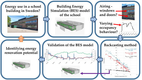
The applied methods in this paper are field measurements, including logged data in Building Management System (BMS), and the utilisation of a BES tool. An overview of the methodology and research process to build and validate the BES model is shown in
Figure 2, and it can be divided into five main steps. In the first step, a vast amount of information during both unoccupied and occupied time periods was collected. Input and validation data were collected from field measurements, BMS logging, and other sources, and the initial BES model was created. The only input data not included in the initial model was the occupants’ airing behaviour. In the second step, the model was validated during an unoccupied time period when no occupants influenced the building. In the third step, a backcasting method on how to model airing and other varying occupancy behaviour was elaborated. The outcome of a function describing airing and occupancy behaviour variations was included as new input data in the model. In the fourth step, the model was validated during an occupied time period. Finally, this model was used to identify potential renovation measures.
Moreover, in steps two, three, and four in
Figure 2, the measured power to the space heating system was compared with simulated data from the model during different time periods, and in step two and four, validation was performed. Validation criteria are set according to ASHRAE Guideline 14 [
25] for discrepancies between measured and simulated hourly data. The Mean Bias Error (MBE) should not be higher than ±10% and Coefficient of Variation of Root Mean Square Error (CV(RMSE)) should not be higher than ±30%.
The strategy adopted to collect input and validation data was done by the evidence-based methodology suggested by Raftery et al. [
23]. Data is categorised in a source hierarchy with the following order of priority: (1) long-term logged data from BMS; (2) field measurements; (3) direct observations and audits; (4) staff interviews; (5) operation documents; (6) construction documents; (7) benchmark studies and best practice guides; (8) standards, specifications and guidelines, and design information. Number one, logged data from BMS, has the highest source hierarchy and number eight (standards, specifications and guidelines, and design information) has the lowest source hierarchy. In Table 5, input and validation data to the model is summarised and the source hierarchy is denoted. Importantly, evidence-based input data with a high source hierarchy are desirable to obtain a reliable and valid model.
3.1. Field Measurements and Logged Data
Electricity and district heat usage provided by the local energy company was merged data for all six school buildings, and no separation between the different buildings was possible. Therefore, sub-metering through field measurements and logging in the BMS was necessary in order to collect input and validation data to the BES model.
Table 2 summarises field measurements, and
Table 3 summarises BMS logging. Both tables specify on which level the data was collected, room level or building level, and if the data were used as input and/or validation data.
Table 4 presents equipment and measurement accuracy. The measurements were mainly performed from December 2014 until April 2015, except for the weather data, which was collected for one whole year.
An extraordinary measurement performed in this project was to quantify air infiltration by measuring the local mean age of air by tracer gas measurements during the non-occupied period [
26]. This unintentional air flow is difficult to capture with other measurement methods and is often unknown input data in BES. The tracer gas measurements also gave proof of why the passive tracer gas method is not suitable in buildings with mechanical AHU systems that have large variations in air flow magnitudes [
33].
Indoor temperatures and electrical equipment baseloads were measured during the non-occupied week with simultaneous inspections. Due to the installation setup, sub-metering of electricity for running HVAC systems and lighting and appliances in common spaces was difficult. Measurements of space heating power and energy in radiator systems were carried out at site with a manufacturer-calibrated TA Scope Premium balancing instrument with two-minute and 10-minute sampling intervals, respectively. A weather station was located on the roof. Temperature, wind speed, and direction from this unit were used to create a weather file in the simulation. The weather station only measured global radiation onto a horizontal surface, while IDA ICE requires diffuse and direct normal radiation onto a normal plane. Thus, complementary data to the weather file was created by using national meteorological weather station data, which were sourced from a station located about 7 km from the studied building and included solar radiation data through STRÅNG and the mesoscale analysis system called MESAN [
34].
3.2. Building Energy Simulation Model Description and Collection of Data
A building model was created in the simulation tool IDA ICE version 4.8. In IDA ICE, thermal indoor climate and energy use can be studied by dynamic multi-zone simulations. IDA ICE has been certified and validated through idealised, empirical, analytical, and peer model validation in recent decades [
35,
36,
37,
38,
39]. A typical simulation required approximately one core hour if performed on an Intel
® Xeon
® CPU E3-1505M v6 @ 3.00GHz computer. The BES simulations were mostly carried out at the University of Gävle’s remote computer servers, Gävle, Sweden. In every simulation, the BES was simulated at least two weeks before the studied validation period in order to diminish initial value problems.
Approximately 100 rooms were modelled as 35 zones. The zoning strategy was done using the zone-typing approach according to Raftery et al. [
23], which includes four major criteria: spatial location to the exterior, function of the space, conditioning methods (e.g., ventilation strategy and set points), and available measurements (including information about internal loads). Rooms were merged into zones in which additional internal mass was included to compensate for internal walls.
3.2.1. Description of Space Heating, Ventilation, and DHW Heating Systems
Space heating, ventilation, and DHW systems are all heated by heat exchangers connected to the local district heating net with an unlimited heat supply. The school is not equipped with cooling devices or air conditioning systems. Input data regarding DHW and DHWC systems are found in
Table 5. Four AHUs with rotary heat exchangers were modelled with heat recovery efficiency based on linear regression on BMS logged data; see
Figure 3. Values below 50% and above 90% were excluded, as these were assumed to be start up and shut down values. The linear function of temperature efficiency as a function of outdoor air temperature was implemented as a control curve into the AHU component models instead of using a fixed value for the efficiency of the rotary heat exchangers.
The AHUs’ supply temperatures were set according to average temperatures logged in the BMS during daytime operation in March 2015; see the input values in
Table 5. Three of the AHUs had fixed schemes; see
Table 5. Presence sensors controlled the fourth AHU, and a generalised scheme was created as described in
Section 3.2.2. The supply and exhaust air flow for each zone are set according to the ventilation inspection protocols for each room. At maximum, the total fan power is about 36 kW, and an air flow of about 10 m
3/s of supply and exhaust air are ventilating the building through all four AHUs.
Hydronic single plane radiators were modelled with emitting capacity from an IDA ICE component library and maximum heat output according to design calculations. Radiators were modelled with proportional thermostats with a dead band of 0.5 °C. Having the control strategy of outdoor compensated supply flow temperature, the heating system has a control curve with a maximum supply temperature of 61.4 °C at an outdoor temperature of −20 °C and a minimum temperature of 19.4 °C at an outdoor temperature of 18 °C. The corresponding curve implemented in the component model is based on the measured radiator circuit’s temperature performance. Night setback decreases the supply temperature by 5 °C between 9:00 and 2:00 the next day Monday to Friday, 24 h during Saturday and until 20:00 during Sunday.
Figure 4 show the supply temperatures control curve over a week with −20 °C outdoor temperature.
3.2.2. Schedules for Internal Loads and Ventilation
For electricity devices, a baseload was measured during the unoccupied time period and was allocated per m
2 area within the whole building and scheduled as “always on”; see the values in
Table 5. For office zones and the coffeehouse, lighting and occupancy were scheduled according to the staffs’ working hours, and the ventilation in these zones was controlled by AHU3. The rooms located at the basement level were ventilated by AHU2 and AHU4; see
Table 5 for schedules for AHU2-4. Lighting in the corridor zones was controlled by a time schedule. The majority of the classrooms were controlled by presence sensors and ventilated by AHU1.
For all zones controlled by presence sensors, a scheme was created for every weekday based on BMS damper positions (10-minute sampling time) of ventilation inlets in 19 rooms. A generalised operation schedule for AHU1, occupants, and lighting was created for these zones.
Figure 5 illustrates a Wednesday schedule, where 1.0 indicates presence control activation in all 19 rooms; 0.0 indicates that no room was used (closed dampers). A half-hourly mean value was created from three typical weeks, and the selection of these weeks was made by studying the measured electricity pattern for the whole building over a whole year.
In total, eight time schedules were created, used, and applied for lighting and occupancy depending on the zone type and functional use and data from BMS. Each of these eight schedules includes specific schemes for each weekday and are adjusted concerning weekend and holiday periods. These schedules can be assumed to capture the overall utilisation of the building in terms of occupants’ presence, use of appliances and devices, and presence-activated ventilation rates. However, this scheme does not capture occupants’ airing due to opening windows, doors, and entrances. Instead, energy losses due to airing, amount of persons, and other unknown energy usage are modelled with the backcasting method described in
Section 3.3. In
Table 5, the input and validation data to the model are summarised. The source hierarchy (described in the end of
Section 2) of the input and validation data is specified in the Assessment method column in
Table 5.
3.3. Validation of the Model—Unoccupied Building
Validation of the model during an unoccupied period was performed during a winter week, from 00:00 on 29 December 2014 to 00:00 on 5 January 2015. The building was fully heated, although occupants were on holiday and all AHUs were intentionally shut off. Validation included comparison between measurements against simulated results at the room and building level: indoor temperatures in three selected validation rooms at the room level, and power and energy for the heating system at the building level. This validation method captures the thermal performance of the building in a more valid and reliable way compared to validation with monthly purchased heat including the heating of space, ventilation, and DHW. Measured and simulated power to the heating system was compared on an hourly basis, and the variation of MBE and CV(RMSE) was calculated. The main purpose at this stage was to validate the building’s thermal performance characteristics without the influence of occupants and occupant-dependent ventilation.
The three rooms that were chosen for validation at the room level were a classroom, a teachers’ office (several teachers share an office), and the staff lunchroom. These rooms were modelled as separate zones and had the same areas in the model as in reality.
Figure 6 illustrates the actual first floor plan.
Figure 7 shows model zoning of the first and second floor and visualises the validation zones: staff lunchroom (a), teachers’ office (b), and classroom (c).
3.4. Modelling Airing and Varying Occupancy Behaviour
Although the activities within the building are to a large extent scheduled and modelled on the basis of ventilation room damper positions as shown in
Figure 5 and described in
Section 3.2.2, there are irregularities which make it difficult to capture the true utilisation of the building in detail. These include the presence of pupils and staff, actual use of reserved rooms/time and activities therein, and equipment utilisation. Moreover, within modelling, a major uncertainty is how to schedule airing in terms of entrances, doors, and windows being opened. Instead of using best practice values for heat losses due to airing or creating schedules for window and door opening based on assumptions, a backcasting method has been developed. Due to occupancy and its consequences, this new method was developed for application to the occupied validation period. The daily mean power difference between measured and modelled heat power to hydronic radiators as a function of mean outdoor temperatures was calculated and a linear regression was applied, see the results in
Section 4.2. The simulated and measured daily mean power was compared during 46 working days between 12 January and 27 March 2015, from 08:00 to 17:00 to study airing and variations in occupancy behaviour. Due to evidence-based input data in the model, it is possible to draw the conclusion that the difference in measured and modelled mean heating power can be attributed mostly to airing activities and other occupant-related energy use in the building, such as the influence of occupancy presence and traffic as well as the use of lighting, equipment, and ventilation. The linear correlation is used as input data and modelled as an extra heat load in the BES model during the validation of an occupied building and when performing a normalised annual BES.
3.5. Validation of the Model—Occupied Building
Validation for the period with the presence of occupants was performed during three months, from 12 January to 5 April 2015. This period represents a validation period including 77 days, 24 h per day of energy use comparison, both regular school weeks and holiday weeks. The linear correlation modelling airing and varying occupancy was included in this simulation. Measured and simulated power to the heating system was compared on an hourly basis, and the variation of MBE and CV(RMSE) was calculated.
3.6. Identification of Energy-Efficiency Measures
After the model was validated during occupied operation, an annual BES during the Swedish heating season, from the middle of September to the middle of May, was performed. A weather file compiled by the Sveby organisation [
42] with typical weather data for the city of Gävle during the years 1981–2010 was applied in the simulation. In this climate file, diffuse and direct solar radiation is calculated through the altitude of the sun, solar angle, cloudiness, and some more parameters [
43]. The heat losses were separated into different posts e.g., windows, external walls, air leakage through construction, etc., the existing
U-values were compared to the Swedish Building Code
U-values (W/(m
2·°C)), and potential energy efficiency measures were identified and discussed.
4. Results
Results from unoccupied and occupied validation periods, how to handle airing and varying occupant behaviour, annual heat balance simulation, and potential energy efficiency measures in renovation planning are presented in this chapter.
4.1. Validation of the Model—Unoccupied Building
Model validation of the unoccupied building includes measurements of space heating at the building level and temperature measurements at the room level. Input data, which might be unknown in BES projects, are for example thermal bridges, infiltration, and other construction data. In this case study, much of the input data is evidence-based data with a high source hierarchy due to detailed data collection and the many field measurements where, for example, infiltration and domestic hot water circulation (DHWC) losses were measured. Validation was performed using both heating power demand and energy use during the above-mentioned week.
4.1.1. Building Level
Figure 8 illustrates measured and simulated heating power demand from the building’s hydronic radiators. In the beginning of the validation period, the outdoor temperature was lower, and both measured and modelled heat power to the radiators were higher and vice versa during the middle of the validation period. An explanation of the higher and more fluctuating measured power during the beginning of the week can depend on air infiltration. In the model, infiltration is set to a fixed average value of 0.12 ACH, which is based on tracer gas measurement during the same period [
26]. In reality, infiltration rates vary with wind conditions and outdoor air temperatures. Discrepancies are also due to initial value problems (since occupancy prior to the non-occupancy period is unknown), differences in control schedules and deficiencies in the building model concerning thermal mass within the building, and in the IDA ICE component models (for example, thermal bridges and the heating system lack thermal inertia).
The time resolution of 15 min mean power, based on measurements sampled every two minutes, shows the difference between measured and modelled heating power in terms of a more fluctuating pattern. This is due to a combination of the non-smooth control of the hydronic valves in the district heating substation, the inertia in the hydronic radiator system caused by the length of the piping, and the inertia in the operation of the radiator thermostats. The IDA ICE component models do not capture quick fluctuations in the heating system.
On 1 January, there was more measured heat power than simulated, which might be explained by the presence of office staff who perhaps were working during some of these holidays, even if the school is assumed to be empty. Since the ventilation systems were off during this week, the present staff might have opened windows due to deficient air quality. This clue was supported by the tracer gas measurements in one of the teachers’ offices during the validation period that indicate windows have been opened in this room [
26].
Figure 9 presents daily differences between measured and simulated energy use. The differences vary between 7.9% and −9.6% and 58 kWh and −139 kWh, where negative values represent higher measured than simulated values. The majority of days show that measured energy use is higher than the simulated use. The summarised measured energy use over the whole week is 7.3 MWh and the simulated energy use is 7.0 MWh. This results in a difference of −3.4%, meaning slightly higher measured energy use compared to simulated use. This difference is less than the accuracy of the measurement equipment. According to ASHRAE Guideline 14 [
25], the difference between measured and simulated data should not be higher than ±10% for MBE and ±30% for CV(RMSE) when using a simulation time step of one hour. This criteria is achieved with a large margin for the unoccupied building; see
Table 6. In this statistical analysis, the outliers that occur during nights, seen as peaks in measured values in
Figure 8, are excluded. The peaks can be explained by the building’s heating control causing an overshoot of heat every night at the time when the supply temperature increases by 5 °C; see the control curve in
Figure 4. This type of overshoot is not modelled by IDA ICE components. In the statistical calculations, one hour of data are excluded every occasion this temperature increase occurs; in total, 5 of 168 values were removed.
In summary, the small differences in heat power demand and energy use might be due to insufficient settings for internal loads in the model such as occupants, use of lights and equipment, and differences in infiltration flows and insolation. Furthermore, in the basement, large heat losses due to partly uninsulated heating pipes exist, which are modelled as ideal heaters in two specific basement zones. There might be a few other parts of the heating energy system that should be covered by the zone radiators rather than by ideal basement heaters (ideal heaters respond perfectly to temperature changes).
Although the total DHWC losses have been measured [
32], it is not known how much of these losses are gained in the building, since two separate buildings share this circulation system. In all simulations, 75% of the DHWC losses are assumed to be gained within the building. A sensitivity analysis concerning DHWC losses as gains varied between 50%, 75%, and 100%. The results from the sensitivity analysis showed that the measured energy use is higher than the simulated energy use. However, the sensitivity analysis shows that the percentage share of DHWC that is assumed to become useful heat in the BES model varies in the three cases between 1.7%, 3.4%, and 5.1%, which is not a critical assumption for the result output.
4.1.2. Room Level
Figure 10 shows indoor temperatures at the room level during the unoccupied validation period. The classroom reveals some peaks where the highest difference is 0.8 °C. The reasons for these variations might depend on insolation, also keeping in mind that IDA ICE zone air temperature is represented by one node (i.e., the room air is totally mixed).
The staff lunchroom located on the east side of the building is not affected by insolation to the same extent as the other rooms, which are located on the west side. However, the teachers’ office is shaded by trees to a larger extent than the classroom. The standard deviation from measured indoor air temperatures is 0.20 °C for the staff lunchroom, 0.19 °C for the teachers’ office, and 0.24 °C for the classroom. The low standard deviation values indicate good correlation between measured and simulated temperatures, and they are within measurement instrument errors.
4.2. Modelling Airing and Varying Occupancy Behaviour
At this stage, the building’s technical characteristics have been validated and tested against measurements for the non-occupied period. The occupancy schemes described in
Section 3.2.2 were implemented, and a three-month period with occupancy was simulated. In
Figure 11, daily mean radiator power, measured (
Pmeasured) and simulated (
Psimulated) heat power to radiators are plotted against daily mean outdoor temperatures for 46 working days (data based on values from 08:00 to 17:00 p.m., 12 January until 27 March 2015). These show outdoor temperature dependency. Moreover, the differences between these two curves are illustrated. The plotted power differences can mostly be ascribed to airing activities by opening doors and windows and other possible behavioural patterns, as described in
Section 3.4, keeping in mind that occupant presence influencing ventilation patterns and human heat emissions have been considered in BES in terms of schedules; see
Section 3.2.2.
The linear correlation for the difference shows an overall power heat loss of 11.46 kW and an additional outdoor temperature dependency term of −0.41 kW/°C. The correlation curve indicates an increase in heating power difference between measured and simulated results as outdoor temperatures become colder. Outdoor temperatures between January and March vary in the same way as outdoor temperatures during autumn. This motivates why this linear correlation can be used to describe the mean power differences over the whole heating season in Sweden, which is often generalised to be from 15 September until 15 May. When performing the validation of an occupied building and during annual simulation with normalised weather data, the linear correlation of daily mean power difference, described in
Figure 11, is added as an extra energy heat loss into the BES model.
4.3. Validation of the Model—Occupied Building
In
Table 7, measured and simulated energy supplied to the radiators are compared during the time period from 12 January to 5 April by encompassing all hours during this period, excluding some days due to a lack of measured data. The monthly differences vary from 5.5% in January, 10.6% in February, and 9.7% in March/April as opposed to the unoccupied period, which resulted in 3.4%. The outliers, caused by the overshoot of heat during night control, are excluded in the same way as for the calculations of the unoccupied period. In the calculations presented in
Table 7 and
Table 8, 54 hourly values are removed from the total values of 1847.
As can be seen in
Table 7, the months of February and March/April might in reality be more divergent compared to the typical school week schedule and because of that, they show larger differences than January. The difference between measured and simulated energy to the space heating system is shown as statistical calculations in
Table 8. The MBE and CV(RMSE) for the occupied period are met according to ASHRAE criteria [
25]; however, the variations are larger for the occupied period compared to the unoccupied period. Some reasons for the observed differences might be the ventilation, light, and occupant schedules. These schedules are generalised and adjusted to represent typical school weeks over the whole year.
4.4. Annual Energy Use for a Typical Year and Identification of Energy Efficiency Measures
The simulated energy balance from the middle of September to the middle of May for heating and domestic hot water use for the school building results in 545 MWh, which represents supplied energy and heat losses, e.g., through the building envelope, ventilation, infiltration, and airing; see
Figure 12. Internal gains contribute 155 MWh of heat, which includes heat from occupants (16 MWh), equipment (74 MWh), and lighting (65 MWh). Purchased district heating includes heating of the hydronic radiator system, the mechanical ventilation system, the DHWC losses, and other pipe heat losses. The heating of DHW is separated from the supplied heat and represents 8 MWh. The total amount of purchased heat is 73 kWh/m
2 for a normalised year.
The heat losses, which are arranged from highest to lowest contribution, are presented in
Table 9. Window transmission losses account for 22% of the total. The second highest losses of 16% are due to infiltration. Future energy efficiency measures could be to replace windows with lower
U values and to air-tighten the building envelope. When renovating a building in Sweden, attempts should be made to fulfil the requirements of the primary energy use, according to the current Swedish building code [
44]. However, if this is not possible, minimum
U-values for small residential houses can be seen as indicative values; see
Table 9 [
44]. It is clear that there is potential in future renovation to achieve lower
U-values when renovating building segment parts. Furthermore, to build a more airtight building envelope will decrease the heat losses due to infiltration losses. The Swedish Forum of Energy Efficient Building (FEBY) set a maximal air leakage of 0.3 l/(s∙m
2) through the building envelope area at a pressure difference of 50 Pa as a criterion in Swedish passive house certification [
45]. The air leakage should be tested according to the standard SS-EN ISO 9972:2015. With a corresponding air tightness of 0.3 l/(s∙m
2 at 50 Pa) pertaining to the enclosing envelope area, the BES results show a heat loss of about 25 MWh due to infiltration. This indicates an extensive reduction of heat loss compared to the current infiltration, which corresponds to 89 MWh during the heating season.
Another large heat loss post is the mechanical ventilation system; see
Table 9. However, the rotary heat exchangers already have high temperature efficiency, as described in
Section 3.2.1. Therefore, possible energy efficiency measures might be to minimise the specific fan power and adjust the air flows. The mechanical ventilation system is an on/off constant air volume (CAV) system controlled by presence sensors; however, the occupancy in the classrooms can vary significantly. Therefore, another control strategy can be a variable air volume (VAV) system controlled by CO
2 and temperature levels. This will reduce the risk of unnecessary air flows and thereby reduce the heat losses. Furthermore, a VAV and CO
2 controlled mechanical ventilation system might also improve the thermal comfort and indoor environment for pupils and staff.
The DHWC losses are simulated as 25% of the heat is lost, which accounts for 8 MWh; see
Figure 12. Measurements on the DHWC together with observations at site visits and thermography pictures showed extensive heat losses through a partly uninsulated hot water piping system. This piping system supplies heat to five other school buildings. However, in the present study, it is not of interest to specify the exact amount of heat emitted from these partly uninsulated pipes, since this heat is assumed to be utilised within the building. However, if looking at the energy use for the whole school, including all six buildings, it is of high interest to decrease these heat losses due to partly uninsulated pipes, especially heat loss in distribution pipes between the buildings. High heating bills during summer holiday periods when the buildings are unoccupied confirms large pipe heat losses.
The heat losses due to airing and other unknown utilisation patterns were simulated to 14 MWh. This corresponds to a value of 3.1 kWh/m
2 per year and represents about 3% of the total amount of purchased district heat. A standard value commonly used for airing losses in BES in Sweden is 4 kWh/m
2 per year [
21], which would result in 18 MWh for the studied building. The simulated energy lost due to airing is thereby somewhat lower than the standard Swedish value for BES simulations. At a glance, the power associated with airing and other variables is about 2.5 W/m
2.
5. Discussion and Conclusions
In this case study, an existing school building was modelled using the building energy simulation tool IDA ICE. The methodology developed in order to create the BES model can be summarised as follows: (1) collect evidence-based input and validation data with majority high source hierarchy; (2) separate validation of occupied and unoccupied time periods, where validation during the unoccupied period specifically concerns the buildings’ technical characteristics; (3) applying a backcasting method in order to compile a heat load that represents airing and varying occupancy behaviour; and (4) perform BES simulation during the heating season to identify renovation potential. This methodology can entirely or partly be applied in other studies when creating BES models of existing buildings, and the ambition is to obtain reliable and validated BES models. The backcasting method can be especially useful to apply when buildings with irregular occupancy behaviour are modelled in BES.
The first objective was to obtain evidence-based input and validation data, and the study shows how the collection of evidence-based data with high source hierarchy, including both logged data in the building management system and detailed field measurements, constitutes a good base to perform validation of the building energy simulation model. This is of especially high importance in case studies including complex buildings such as school buildings. A strength of the study was the many field measurements providing input data, which often are unknown in BES case studies, such as for example infiltration leakage, which was measured through passive tracer gas measurements. Hot water circulation losses and space heating power were also measured and the performance of thermal bridges was calculated.
The second objective was to perform a separate validation of unoccupied and occupied time periods. The unoccupied period enables validation of the building thermal performance when uncertainties connected to occupancy behaviour input data are not present. The results from the unoccupied validation period show that the building’s thermal performance is correctly modelled with only a discrepancy of 3.4% difference of simulated and measured heat to the hydronic radiators during one week. Furthermore, measurements of 15-min resolution capture the minor differences in simulated and measured operation of the heating system. Sensitivity analysis on the percentage of DHWC, which is gained as heat in the building, showed that this is not critical input data. At the room level, measured and simulated indoor temperatures in three validation rooms showed good agreement with a standard deviation of only 0.19–0.24 °C.
The third objective was fulfilled by the development of a backcasting method. As highlighted in the introduction, the airing and opening of windows and doors are often unknown input data that are difficult to model in BES. In this study, the energy loss due to airing and varying occupant behaviour was elaborated using a backcasting method. In this method, airing heat loss is modelled by creating a linear correlation including the daily mean power difference between measured and simulated heat to the hydronic radiators and outdoor temperature during 46 workdays, January to March, between 08:00 and 17:00. The result showed a mean power heat loss of 11.5 kW and additional outdoor temperature correlation of −0.41 kW/°C. This linear correlation was used as input data to represent varying occupancy behaviour and the majority of airing activities during the Swedish heating season from September to May. The linear correlation was implemented into the model and used in both validation of the occupied building and in the annual heat balance simulation. The annual heat loss due to airing was predicted at 14 MWh, corresponding to 3.1 kWh/m2 and year and implying an overall power loss of 2.1 W/m2 during working hours/use of the school. Validation of the model during occupied time periods resulted in monthly discrepancies between measured and simulated energy use for space heating varying between 5.5% and 10.6% during three months. This can be seen as an acceptable discrepancy for a valid BES model during an occupied period. It was more important that this model contains schedules of occupancy behaviour and mechanical ventilation operation that represent typical behaviour during the whole year than to calibrate or “tune” the model to achieve a perfect match between measurement and simulations during a specific time period. This backcasting method is a suitable complement to the strategy of generating schedules for room ventilation and internal loads based on the presence of controlled ventilation damper positions.
Validating the BES model and handling modelling uncertainties are preconditions to fulfil the final goal with the modelling: to perform as accurate and realistic a prediction of the real system modelled as possible. In this case study, the final BES model predicts a total need of purchased heat at 73 kWh/m2, 332 MWh in the school building. The fourth objective was to identify energy-efficiency measures, and the ones that have the greatest impact on energy use (in order of highest first) were changing to energy-efficient windows, improved airtightness of the building envelope (which corresponds to 0.12 ACH), new controls of the HVAC system, and increased wall insulation. In future research, the validated model will be used for investigations on life-cycle cost optimisation of energy-efficient measures in renovation planning.
Author Contributions
Conceptualisation, J.S.E., M.C., J.A. and B.M.; Data curation, J.S.E.; Formal analysis, J.S.E., M.C., J.A. and B.M.; Funding acquisition, B.M.; Investigation, J.S.E. and J.A.; Methodology, J.S.E., M.C., J.A. and B.M.; Project administration, J.S.E.; Software, J.S.E. and J.A.; Supervision, M.C., J.A. and B.M.; Validation, J.S.E., M.C., J.A. and B.M.; Visualisation, J.S.E.; Writing—original draft, J.S.E.; Writing—review and editing, J.S.E., M.C., J.A. and B.M. All authors have read and agreed to the published version of the manuscript.
Funding
This research was funded by Gavlefastigheter AB, and the Knowledge Foundation (KK-stiftelsen) grant number 20120273.
Acknowledgments
The work has been carried out under the auspices of the industrial post-graduate school Reesbe, which is financed by the Knowledge Foundation (KK-stiftelsen).
Conflicts of Interest
The authors declare no conflict of interest.
References
- International Energy Agency. Energy Technology Perspectives—Scenarios and Strategies to 2050; International Energy Agency: Paris, France, 2010. [Google Scholar]
- Pérez-Lombard, L.; Ortiz, J.; Pout, C. A review on buildings energy consumption information. Energy Build. 2008, 40, 394–398. [Google Scholar] [CrossRef]
- European Council. EUCO 169/14—Conclusions 23/24 October 2014; European Council: Brussels, Belgium, 2014. [Google Scholar]
- European Council. Directive 2010/31/EU of the European Parliament and of the Council of 19th May on the energy performance of buildings. In Directive 2010/31/EU, DOUE 153; European Council: Brussels, Belgium, 2010. [Google Scholar]
- European Council. EED Directive 2012/27/EU of the European Parliament and of the Council of 25 October 2012 on energy efficiency. In 2012/27/EU; European Council: Brussels, Belgium, 2012. [Google Scholar]
- Coakley, D.; Raftery, P.; Keane, M. A review of methods to match building energy simulation models to measured data. Renew. Sustain. Energy Rev. 2014, 37, 123–141. [Google Scholar] [CrossRef]
- Fabrizio, E.; Monetti, V. Methodologies and Advancements in the Calibration of Building Energy Models. Energies 2015, 8, 2548–2574. [Google Scholar] [CrossRef]
- Ryan, E.M.; Sanquist, T.F. Validation of building energy modeling tools under idealized and realistic conditions. Energy Build. 2012, 47, 375–382. [Google Scholar] [CrossRef]
- Sunikka-Blank, M.; Galvin, R. Introducing the prebound effect: The gap between performance and actual energy consumption. Build. Res. Inf. 2012, 40, 260–273. [Google Scholar] [CrossRef]
- De Wilde, P. The gap between predicted and measured energy performance of buildings: A framework for investigation. Autom. Constr. 2014, 41, 40–49. [Google Scholar] [CrossRef]
- Gaetani, I.; Hoes, P.-J.; Hensen, J.L. Occupant behavior in building energy simulation: Towards a fit-for-purpose modeling strategy. Energy Build. 2016, 121, 188–204. [Google Scholar] [CrossRef]
- Hoes, P.; Hensen, J.; Loomans, M.; De Vries, B.; Bourgeois, D. User behavior in whole building simulation. Energy Build. 2009, 41, 295–302. [Google Scholar] [CrossRef]
- Yang, J.; Santamouris, M.; Lee, S.E. Review of occupancy sensing systems and occupancy modeling methodologies for the application in institutional buildings. Energy Build. 2016, 121, 344–349. [Google Scholar] [CrossRef]
- Dong, B.; Yan, D.; Li, Z.X.; Jin, Y.; Feng, X.H.; Fontenot, H. Modeling occupancy and behavior for better building design and operation-A critical review. Build. Simul. 2018, 11, 899–921. [Google Scholar] [CrossRef]
- Yan, D.; O’Brien, W.; Hong, T.; Feng, X.; Gunay, H.B.; Tahmasebi, F.; Mahdavi, A. Occupant behavior modeling for building performance simulation: Current state and future challenges. Energy Build. 2015, 107, 264–278. [Google Scholar] [CrossRef]
- Haldi, F.; Robinson, D. Interactions with window openings by office occupants. Build. Environ. 2009, 44, 2378–2395. [Google Scholar] [CrossRef]
- Fabi, V.; Andersen, R.V.; Corgnati, S.; Olesen, B.W. Occupants’ window opening behaviour: A literature review of factors influencing occupant behaviour and models. Build. Environ. 2012, 58, 188–198. [Google Scholar] [CrossRef]
- Pisello, A.L.; Castaldo, V.L.; Piselli, C.; Fabiani, C.; Cotana, F. How peers’ personal attitudes affect indoor microclimate and energy need in an institutional building: Results from a continuous monitoring campaign in summer and winter conditions. Energy Build. 2016, 126, 485–497. [Google Scholar] [CrossRef]
- Dutton, S.; Shao, L. Window opening behaviour in a naturally ventilated school. In Proceedings of the Simbuilt 2010, New York, NY, USA, 11–13 August 2010; pp. 260–268. [Google Scholar]
- Zhang, Y.; Bai, X.; Mills, F.P.; Pezzey, J.C. Rethinking the role of occupant behavior in building energy performance: A review. Energy Build. 2018. [Google Scholar] [CrossRef]
- Sveby. Brukarindata Undervisningsbyggnader version 1.0; Svebyprogramet: Stockholm, Sweden, 2016; Available online: http://www.sveby.org (accessed on 14 November 2019).
- Moran, P.; Hajdukiewicz, M.; Goggins, J. Achieving Nearly Zero Energy Buildings-A Lifecycle Assessment Approach to Retrofitting Buildings. In Proceedings of the Advanced Building Skins, At Graz, Austria, 23–24 April 2015. [Google Scholar]
- Raftery, P.; Keane, M.; O’Donnell, J. Calibrating whole building energy models: An evidence-based methodology. Energy Build. 2011, 43, 2356–2364. [Google Scholar] [CrossRef]
- International Standard ISO 13370:2017. Thermal performance of buildings—Heat transfer via the ground—Calculation methods. International Organization for Standardization: Geneva, Switzerland, 2017.
- Ashrae, G. Guideline 14-2002. In Measurement of Energy and Demand Savings; American Society of Heating, Ventilating, and Air Conditioning Engineers: Atlanta, Georgia, 2002. [Google Scholar]
- Steen Englund, J.; Akander, J.; Björling, M.; Moshfegh, B. Assessment of Airflows in a School Building with Mechanical Ventilation Using Passive Tracer Gas Method. In Mediterranean Green Buildings & Renewable Energy; Sayigh, A., Ed.; Springer: Cham, Switzerland, 2017; pp. 619–631. [Google Scholar] [CrossRef]
- Mitech Instrument. Mitec SatelLite-TH. Available online: http://www.mitec.se/sv/produkter_dataloggrar_kompaktloggrar.html (accessed on 11 November 2019).
- IMI Hydronic. TA-SCOPE Instrument. Available online: https://www.imi-hydronic.com/sites/EN/international/products/balancing-control-actuators/measuring-tools/instruments/TA-SCOPE/170c70d5-5229-4e20-8058-1501fdfbca15 (accessed on 10 November 2019).
- Gemini Data Loggers. Tinytag Energy logger. Available online: https://www.geminidataloggers.com/data-loggers/tinytag-energy-data-logger (accessed on 7 November 2019).
- Davis Instruments. Vantage Pro. Available online: https://www.davisinstruments.com/weather-monitoring/ (accessed on 11 November 2019).
- Fuji Electric. Portable Flowmeter Fuji Portaflow X. Available online: https://www.coulton.com (accessed on 13 November 2019).
- Salazar Navalón, P. Evaluation of Heat Losses from a Domestic Hot Water Circulation System. MSC Thesis, University of Gävle, Gävle, Sweden, 2015. [Google Scholar]
- Björling, M.; Akander, J.; Steen Englund, J. On Measuring Air Infiltration Rates Using Tracer Gases in Buildings with Presence Controlled Mechanical Ventilation Systems. In Proceedings of the Indoor Air 2016, 14th International Conference of Indoor Air Quality and Climate, Ghent, Belgium, 3–8 July 2016. [Google Scholar]
- Lundström, L. Shiny weather data. Available online: https://rokka.shinyapps.io/shinyweatherdata/ (accessed on 5 May 2019).
- Equa Simulation AB. Validation of IDA Indoor Climate and Energy 4.0 build 4 with respect to ANSI/ASHRAE Standard 140-2004; EQUA Simulation Technology Group: Stockholm, Sweden, 2010. [Google Scholar]
- Equa Simulation AB. Validation of IDA Indoor Climate and Energy 4.0 with respect to CEN Standard EN 15255-2007 and EN 15265-2007; EQUA Simulation Technology Group: Stockholm, Sweden, 2010. [Google Scholar]
- Kropf, S.; Zweifel, G. Validation of the Building Simulation Program IDA-ICE According to CEN 13791 “Thermal Performance of Buildings–Calculation of Internal Temperatures of a Room in Summer Without Mechanical Cooling–General Criteria and Validation Procedures”; Hochschule fur Technik+ Architektur Luzern: Horw, Switzerland, 2001. [Google Scholar]
- Loutzenhiser, P.; Manz, H.; Maxwell, G. Empirical validations of shading/daylighting/load interactions in building energy simulation tools; Technical Report; Swiss Federal Laboratories for Materials Testing and Research: Duebendorf, Switzerland; Iowa State University: Ames, IA, USA, 2007. [Google Scholar]
- Moosberger, S. IDA-ICE CIBSE-validation, Test of IDA Indoor Climate and Energy version 4.0 according to CIBSE TM33, issue 3; Hochschule fur Technik+ Architektur Luzern: Horw, Switzerland, 2007. [Google Scholar]
- International Standard ISO 10211:2007. Thermal Bridges in Building Construction–Heat Flows and Surface Temperatures–Detailed Calculations; International Organization for Standardization: Geneva, Switzerland, 2007. [Google Scholar]
- International Standard ISO 16000-8:2007. Indoor air—Part 8: Determination of local mean ages of air in buildings for characterizing ventilation conditions; International Organization for Standardization: Geneva, Switzerland, 2007. [Google Scholar]
- Levin, P. Klimatdatafiler Sveby SMHI 1981-2010. Svebyprogrammet 2016. Available online: www.sveby.org (accessed on 22 August 2019).
- Taesler, R.; Andersson, C.J.E. Method for solar radiation computations using routine meteorological observations. Energy Build. 1984, 7, 341–352. [Google Scholar] [CrossRef]
- National Board of Housing Building and Planning. Boverkets Byggregler—föreskrifter och allmänna råd, BBR 26—BFS 2018:4. Available online: https://www.boverket.se/ (accessed on 4 December 2019).
- Forum för Energieffektivt byggande. FEBY 18—Kravspecifikation för energieffektiva byggnader- bostäder och lokaler. Available online: https://www.feby.se/ (accessed on 4 December 2019).
Figure 1.
The school building, 97 m length, 18 m width, and 9 m height above the ground and the building energy simulation (BES) model, including shading objects such as trees shown in (a) and in (b) in form of screens.
Figure 1.
The school building, 97 m length, 18 m width, and 9 m height above the ground and the building energy simulation (BES) model, including shading objects such as trees shown in (a) and in (b) in form of screens.
Figure 2.
Overview of the research process.
Figure 2.
Overview of the research process.
Figure 3.
Linear correlation of rotary heat exchanger temperature efficiency in AHU and outdoor temperature; data set 1 September 2014 until 31 May 2015 (sampled every 10 min).
Figure 3.
Linear correlation of rotary heat exchanger temperature efficiency in AHU and outdoor temperature; data set 1 September 2014 until 31 May 2015 (sampled every 10 min).
Figure 4.
Hydronic radiator supply temperature schedule a week with −20 °C outdoor temperature.
Figure 4.
Hydronic radiator supply temperature schedule a week with −20 °C outdoor temperature.
Figure 5.
Schedule for Wednesday, classrooms in a normal school week, based on damper positions.
Figure 5.
Schedule for Wednesday, classrooms in a normal school week, based on damper positions.
Figure 6.
The actual rooms in the first floor plan.
Figure 6.
The actual rooms in the first floor plan.
Figure 7.
Top picture shows the zoning in the first floor in the model, including the validation zone staff lunchroom (a). Bottom picture shows the zoning in the second floor, including the validation zones teachers’ office (b) and classroom (c).
Figure 7.
Top picture shows the zoning in the first floor in the model, including the validation zone staff lunchroom (a). Bottom picture shows the zoning in the second floor, including the validation zones teachers’ office (b) and classroom (c).
Figure 8.
Measured (blue line) and simulated (red line) energy to the hydronic radiators and outdoor temperature (green line) during the unoccupied validation period.
Figure 8.
Measured (blue line) and simulated (red line) energy to the hydronic radiators and outdoor temperature (green line) during the unoccupied validation period.
Figure 9.
Measured (blue) and simulated (red) energy to the hydronic radiators per day including the difference percentage between measured and modelled energy during the unoccupied validation period.
Figure 9.
Measured (blue) and simulated (red) energy to the hydronic radiators per day including the difference percentage between measured and modelled energy during the unoccupied validation period.
Figure 10.
Measured (blue line) and simulated (red line) indoor temperatures in the three validation rooms, staff lunchroom (a), teachers’ office (b), and classroom (c) during the unoccupied validation period and location of the validation zones at building floorplans (d).
Figure 10.
Measured (blue line) and simulated (red line) indoor temperatures in the three validation rooms, staff lunchroom (a), teachers’ office (b), and classroom (c) during the unoccupied validation period and location of the validation zones at building floorplans (d).
Figure 11.
Mean power difference between measured and modelled heat power to hydronic radiators as a function of outdoor temperature daily values.
Figure 11.
Mean power difference between measured and modelled heat power to hydronic radiators as a function of outdoor temperature daily values.
Figure 12.
Heat balance of the school building, simulated during heating season, 1 September to 31 May, with normalised climate data.
Figure 12.
Heat balance of the school building, simulated during heating season, 1 September to 31 May, with normalised climate data.
Table 1.
Building construction description.
Table 1.
Building construction description.
| Building Segment | Area (m2) | U-Value (W/(m2·°C)) |
|---|
| Roof | 1700 | 0.15 |
| Walls above ground | 1579 | 0.32 1 |
| Walls below ground | 471 | 0.50 1 |
| Floor towards ground | 1700 | 0.22 2 |
| Windows | 465 | 2.7 |
| Total | 5956 | 0.51 |
Table 2.
Overview of measurements.
Table 2.
Overview of measurements.
| Measurements | Measuring at Level | Use of Data |
|---|
| | Room | Building | Model Input | Model Validation |
|---|
| Tracer gas for air leakage | X | | X | |
| Room air temperature | X | | X | X |
| Space heating power | | X | | X |
| Electric baseload power | | X | X | |
| Weather data | | X | X | |
| DHWC 1 | | X | X | |
Table 3.
Overview of Building Management System (BMS) logging.
Table 3.
Overview of Building Management System (BMS) logging.
| BMS Logging | Logging at Level | Use of Data |
|---|
| | Room | Building | Model Input | Model Validation |
|---|
| Damper positions 1 | X | | X | |
| Air temperatures in AHU 2 | | X | X | |
| AHU efficiency 3 | | X | X | |
Table 4.
Measurement equipment and accuracy.
Table 4.
Measurement equipment and accuracy.
| Measurements | Equipment | Accuracy |
|---|
| Tracer gas for air leakage 1 | Passive sources and samplers | Total uncertainty of ±20% within 95% confidence interval [26]. |
| Room air temperature | Mitec SatelLite-TH devices | Inaccuracy of ±0.4 °C for temperature [27]. |
| Space heating power | TA Scope Premium | Inaccuracy of approx. ±5% of flow and ˂±0.2 °C of temperature [28]. |
| Electric baseload | Tinytag Energy loggers | Inaccuracy of ± 2% [29] |
| Weather data | Vantage Pro2 | Temperature inaccuracy of ±0.5 °C [30]. |
| DHWC | Ultrasonic flowmeter Portaflow X | For pipe size ⌀ 13 to 50 mm, inaccuracy of 1.5% of flow rate (between 2 to 32 m/s) and 0.03 m/s (between 0 to 2 m/s) [31]. See also [32]. |
Table 5.
Input and validation data overview. Values, source of collected data, and comments.
Table 5.
Input and validation data overview. Values, source of collected data, and comments.
| Parameter/Variable | Role | Value | Assessment Method 1 | Comment |
|---|
| Areas | Input | See Table 1 | (3) (6) | Main measures checked with measurements. |
Construction
U-values | Input | See Table 1 | (3) (6) | External walls had additional insulation, which was not updated in drawings but was estimated and measured at site. Material properties applied according to IDA ICE database. |
| Windows | Input | g-value 0.76 | (3) (6) (7) | Window types with double glazing were observed and g-value assumed according to the BES tool ICA ICE database. |
| Solar shading | Input | Yes
g-value 0.39 | (3) (7) | Blind between window panes. Regulated by schedule and at insolation of 100 W/m2 or more and multiplier for g-value according to the IDA ICE database. |
| Thermal bridges | Input | 416 W/K | (6) and calculation | Total heat loss coefficient established by using Comsol Multiphysics 3.5. Typical thermal bridges were identified and modelled according to ISO 10211:2007 [40] and thermography.
|
| Building air leakage | Input | 0.12 ACH | (2) | Passive tracer gas method to measure average ACH for the whole building [26,33,41]. |
| AHU flow rates | Input | 4.25–0.55
l/s, m2 | (5) | From ventilation inspection protocols. |
| AHU supply air temp | Input | 17.8–18.5 °C | (1) | Mean value of supply air temp. AHU1 = 18 °C, AHU2 = 17.8 °C, AHU3 = 18.5 °C, AHU4 = 18 °C. Assumed inaccuracy of ±0.5 °C for BMS logging. |
| AHU1 scheme | Input | 1 schedule | (1) | Generalised schedule from three typical school weeks based on logged data of damper positions in room ventilation inlets. See Figure 5 and text Section 3.2.2 for description. |
| AHU2-4 schemes | Input | 3 schedules | (5) | AHU2 = On 7:45 to 15:45 working days, AHU3 = On 6:30 to 17:30 working days, AHU4 = On 7:00–16:00 working days |
| AHU heat exchanger efficiency | Input | Control curve | (1) | Linear regression to model component performance in BES, based on logged data of AHU heat exchanger efficiency. See Figure 3 and text Section 3.2.1 for description. |
| Radiator system, design, and control | Input | Control curve | (5) (6) | Design heat power according to construction drawings and implemented as a component model within the BES model. Control curve according to BMS documentation. See Figure 4 and the text of Section 3.2.1 for a description. |
| Radiator system, space heating | Validation | See Section 3.1, Section 4.1.1, Section 4.2, and Section 4.3 | (2) | Measurements of power and energy in radiator system. See Table 2 and Table 4 and the text in Section 3.1 for a technical description. See Section 4.1.1, Section 4.2, and Section 4.3 for how measurements were used in the validation and backcasting method. |
| Indoor set-point temperatures | Input Indoor set-point temperaturesValidation | 17.1–22.3 °C | (2) | See Table 2 and Table 4 and the text in Section 3.1 for technical description. See Section 4.1.2 for how the measurements have been used in validation. |
| Electric baseload | Input | 1.75 W/m2 | (2) (3) | Audits at site were done to map the location of the loads. See Table 2 and Table 4 and the text in Section 3.1 for a technical description. |
| Lighting in zones | Input | 8.4–15.6 W/m2 | (3) | Lighting power in different rooms is documented during the audits at site. See the text in Section 3.2.2 for a description of schedules. |
| Weather data | Input | Prn. File | (2) | Local weather prn file created from measurement data from the local weather station on roof and the national meteorological weather station. The weather file was used in both the validation and backcasting method. See Table 2 and Table 4 and Section 3.1 for a technical description. |
| Domestic hot water use | Input | 2 kWh/m2, year | (8) | Swedish standard Sveby [21]. |
| Domestic hot water circuit losses | Input | 1 W/m2 | (2) | Ultrasonic flow measurements, see the Master’s thesis for more details [32]. Most (75%) of the heat is assumed to be useful heat inside the building construction. |
| Occupant number | Input | 0.038 occup./m2 | (4) | No. of occupants based on interviews and class schedules. In total, 160 occupants: 140 pupils and 20 staff. |
| Utilisation schedules | Input | 8 varying schedules | (1) (5) | See Figure 5 and Section 3.2.2 for a description. |
| Airing | Input | See Section 3.4 and 4.2 | (2) | Air leakage through windows, doors, and entrance openings. Backcasting method compiled; see Section 3.4 and 4.2 for a description. |
Table 6.
Differences between simulated and measured energy to the hydronic radiators. One week hourly data, 29 December 2014 to 5 January 2015.
Table 6.
Differences between simulated and measured energy to the hydronic radiators. One week hourly data, 29 December 2014 to 5 January 2015.
| Measured Energy Use | Simulated Energy Use | MBE Hourly Data | CV(RMSE) Hourly Data |
|---|
| (MWh) | (MWh) | (%) | (%) |
|---|
| 7.3 | 7.0 | 3.3 | 14.2 |
Table 7.
Monthly measured and simulated energy to the hydronic radiators, including the difference in energy and percentage during the occupied validation period.
Table 7.
Monthly measured and simulated energy to the hydronic radiators, including the difference in energy and percentage during the occupied validation period.
| | Measured Energy Use | Simulated Energy Use | Difference | Difference Percentage |
|---|
| (MWh) | (MWh) | (MWh) | (MWh) |
|---|
| January | 20.1 | 19.0 | 1.1 | 5.5 |
| February | 32.4 | 29.0 | 3.4 | 10.6 |
| March/April | 26.3 | 23.7 | 2.5 | 9.7 |
Table 8.
Differences between simulated and measured energy to the hydronic radiators. Hourly values for three-month occupied time period, January to April 2015.
Table 8.
Differences between simulated and measured energy to the hydronic radiators. Hourly values for three-month occupied time period, January to April 2015.
| Measured Energy Use | Simulated Energy Use | MBE Hourly Data | CV(RMSE) Hourly Data |
|---|
| (MWh) | (MWh) | (%) | (%) |
|---|
| 78.8 | 71.7 | 9.0 | 28.8 |
Table 9.
Distribution of heat losses in heat balance, simulated during the heating season, 1 September to 31 May, with normalised climate data.
Table 9.
Distribution of heat losses in heat balance, simulated during the heating season, 1 September to 31 May, with normalised climate data.
| Title 1 | Heat Loss | Percentage | Existing Building U-Value | Swedish Building Code U-Value [44] |
|---|
| (MWh) | (W/(m2·°C)) | (W/(m2·°C)) |
|---|
| Windows | 145 | 27% | 2.7 | 1.2 |
| Infiltration | 89 | 16% | - | - |
| Mechanical ventilation | 87 | 16% | - | - |
| Walls | 81 | 15% | 0.36 1 | 0.18 |
| Thermal bridges | 49 | 9% | 416 2 | - |
| Floor | 35 | 6% | 0.22 | 0.15 |
| Roof | 28 | 5% | 0.15 | 0.13 |
| Airing and unknown utilisation | 14 | 3% | - | - |
© 2020 by the authors. Licensee MDPI, Basel, Switzerland. This article is an open access article distributed under the terms and conditions of the Creative Commons Attribution (CC BY) license (http://creativecommons.org/licenses/by/4.0/).


