The Key Factors That Determine the Economically Viable, Horizontal Hydrofractured Gas Wells in Mudrocks

Abstract

We assemble a multiscale physical model of gas production in a mudrock (shale). We then tested our model on 45 horizontal gas wells in the Barnett with 12–15 years on production. When properly used, our model may enable shale companies to gain operational insights into how to complete a particular well in a particular shale. Macrofractures, microfractures, and nanopores form a multiscale system that controls gas flow in mudrocks. Near a horizontal well, hydraulic fracturing creates fractures at many scales and increases permeability of the source rock. We model the physical properties of the fracture network embedded in the Stimulated Reservoir Volume (SRV) with a fractal of dimension $D<2$. This fracture network interacts with the poorly connected nanopores in the organic matrix that are the source of almost all produced gas. In the practically impermeable mudrock, the known volumes of fracturing water and proppant must create an equal volume of fractures at all scales. Therefore, the surface area and the number of macrofractures created after hydrofracturing are constrained by the volume of injected water and proppant. The coupling between the fracture network and the organic matrix controls gas production from a horizontal well. The fracture permeability, $k_f$, and the microscale source term, s, affect this coupling, thus controlling the reservoir pressure decline and mass transfer from the nanopore network to the fractures. Particular values of $k_f$ and s are determined by numerically fitting well production data with an optimization algorithm. The relationship between $k_f$ and s is somewhat hyperbolic and defines the type of fracture system created after hydrofracturing. The extremes of this relationship create two end-members of the fracture systems. A small value of the ratio $k_f/s$ causes faster production decline because of the high microscale source term, s. The effective fracture permeability is lower, but gas flow through the matrix to fractures is efficient, thus nullifying the negative effect of the smaller $k_f$. For the high values of $k_f/s$, production decline is slower. In summary, the fracture network permeability at the macroscale and the microscale source term control production rate of shale wells. The best quality wells have good, but not too good, macroscale connectivity.

1. Significance Statement

Our earlier scaling analysis of the Barnett gas play [1,2,3], as well as the unpublished analyses of the Fayetteville and Haynesville plays, revealed that ultimate recovery factors in shales scale as

$$\mathrm{R}\mathrm{F}=\frac{{\mathcal{M}}_{\mathrm{stimulated}}}{{\mathcal{M}}_{\mathrm{geometric}}^a}$$

(1)

where $\mathrm{R}\mathrm{F}$ is the recovery factor, ${\mathcal{M}}_{\mathrm{stimulated}}$ is the mass of produced gas in the stimulated reservoir volume (SRV) in mudrock, and ${\mathcal{M}}_{\mathrm{geometric}}^a$ is the mass of gas initially present in an imaginary parallelepiped enclosing the well and its hydrofractures. The power exponent a sharply less than one (see Figure 1). ${\mathcal{M}}_{\mathrm{geometric}}$ depends on the height of the hydrofracture and the distance between two hydrofracture planes. Notice that the mudrock volumes around the Barnett wells are better connected than those in the Haynesville. This power law behavior is in stark contrast to recovery factors in conventional reservoirs, where $a=1$. Notice that ${\mathcal{M}}_{\mathrm{geometric}}^a\ll {\mathcal{M}}_{\mathrm{geometric}}$, when $a<1$. Therefore, ${\mathcal{M}}_{\mathrm{stimulated}}$ in unconventional reservoirs must be much less than that in conventional ones. We conclude that the stimulated reservoir volumes connected to wells in shales have self-similar (or fractal) flow properties over multiple scales. This observation is the key motivation for the proposed multiscale model of gas production from shale wells.

After two years of uninspiring oil and gas prices that may remain low for several years, “a new era of moderation for shale producers” has emerged as companies focus on capital discipline and shareholder returns [4]. This realignment of shale companies is driven by the worsening access to capital and the forced cuts of capital spending in excess of 20% between 2019 and 2021. Starting from 2019, the industry must guarantee that only the better and cheaper wells be drilled and completed in shales. A mixture of numerical modeling of well production and of data analytics, exemplified by the hyperbolic decline curve analysis (DCA), as shown in Figure 2a and Figure 3, are the industry’s prevailing response (e.g., [5]) to the imploding capital spending. Recently, academia stepped in with a better DCA approach [6] and a hybrid of physical and statistical scaling of field data for thousands of gas wells [1,2,3,7,8] and of oil wells [9,10,11,12] (see Figure 2b. The hybrid approach to scaling production of all fractured, sometimes refractured, pumped off or not, horizontal wells in shales is superior to current industry standards. However, this approach is more complicated and its diffusion into the industry will take a while.

Today, we can scale individually the past performance of tens of thousands of producers in all shale plays, and predict their future performance with reasonable certainty. We can glean the impacts of lateral length, number of hydrofracture stages, architecture of clusters, etc. on the overall performance of these wells [3,11,12]. However, the integrated multiscale model developed in this paper can inform the more detailed operational decisions about the interactions of geology and reservoir parameters with the number of perforation clusters, the number of perforations per cluster, cluster spacing, the size of hydrofracturing jobs, complexity of the stimulated reservoir volume, etc. Most elements of this model are not new, but how they are integrated to optimize well performance in a gas shale is new to our knowledge.

2. Introduction

In several other papers, we performed extensive literature reviews of DCA applied to shale wells, [1,2,3,8,11,12,18,19], and we do not repeat them here. It suffices to say that Figure 2 captures quite clearly the quantitative differences between curve fitting of production rates from shale wells (hyperbolic fits) and physics-based scaling of the same production. Time on production in Figure 2 increases along the diagonal away from the origin. The volume of gas produced during each successive year on production for each well is coded with an increasingly hot color. For the reasons explained in [12], hyperbolic DCA is systematically biased towards exaggeration of production rates from shale wells, especially later in their lifetimes. There have been numerous successful efforts to improve the ability of DCA to capture different flow regimes in shales, notably the three-segment DCA approach that provides 95% accuracy [6,20]. With the wealth of the displayed data (∼100,000 points), one can clearly notice that the patches of the hotter colors (later years on production) are larger for the hyperbolic DCA, meaning that the late-time production rates are too high in most of the wells. In addition, the cloud of points for the hyperbolic DCA diffuses away from the diagonal more than that for the physical scaling, meaning that the goodness of fit (the $R^2$ coefficient) is lower. In short, in a data-driven analysis, physics-based scaling always works better than pure curve fits. It has a higher predictive power [3]. The purpose of this paper is to improve further the quality of a two-parameter scaling of gas production ($\tau ,\mathcal{M}$, see [1]) by invoking a richer multi-scale physics of gas flow in shales. We abbreviate the current model as the $k_f,s,D$ model. Notice that the original mass in place, $\mathcal{M}$, and effective spacing of active fractures, d, also enter the current model.

Organic matter, natural fractures, and hydrofracture-induced fractures create multiscale connectivity that releases gas from the nanopores and enables gas production from mudrocks. In the mudrocks in thermally mature basins, most of the pores develop in the organic matter [21] with an increase in pressure and temperature in the subsurface. With an increase in thermal maturity, local connectivity of organic pores also increases and the dominant pore size that emerges is 2–50 nm [22,23,24,25]. These pores tend to become larger as the source rock matures. Organic matter that hosts most of the nanopores exists as thin laminations in mudrocks and acts as the major source of gas production. High local connectivity [26,27,28] of these nanopores is the characteristic property of the kerogen specks. Contacts between the organic matter and the inorganic matter in these shales are the surfaces of mechanical weakness that are stimulated after hydrofracturing and expose nanopores to high permeability pathways. Berthonneau et al. [29] showed that the largest pores are the potential crack areas at those weakness surfaces. These cracks create multiscale connectivity even at the pore scale. The smallest nanopores (radius ∼1 nm) transfer gas to the larger pores, which eventually connect to the fracture network.

Hydrocarbon production in shales starts after a rapid, orders of magnitude permeability increase from rock stimulation by hydrofracturing. Interpretation of microseismic event magnitudes and spatial distribution during/after hydrofracturing implies the development of a complex network of fractures that branch in multiple directions and have a wide range of lengths from microns to meters. These fracture networks—that consist of induced fractures and reactivated natural fractures (that slip in shear and/or reconnect in tension and may be propped)—create a percolating backbone flow network, increase rock permeability, and drain gas from the organic matrix. The fracture network in contact with the organic matrix is referred as the Stimulated Reservoir Volume (SRV). The part of the stimulated reservoir volume, which is well-connected and produces gas at the reservoir-scale is the Effective Propped Volume (EPV). The authors of [30,31,32,33] showed that outside of the SRV, there exists an unstimulated matrix, whose flow contribution is negligible over a period of 20–25 years, because of its very low permeability. However, the authors of [8,30,34,35,36,37] showed a potentially considerable effect of the unstimulated matrix during 30 years of production from a gas well.

In this study, the stimulated reservoir volume is assumed to have fractal properties. The fractals that quantify heterogeneity of properties of the naturally fractured reservoirs were introduced by Chang et al. [38] and Acuna et al. [39]. Figure 4 is a schematic representation of a fractal porous medium. Fractures are initiated along the line passing through the center of cylinder. Away from the cylinder’s center, toward the outer surface, fracture density decreases according to a power law. Chang et al. [38] derived variation of fracture properties in a differential shell containing a fractal fracture network. The original equations were simplified by Acuna et al. [39] and presented as:

$$\varphi \left(x\right)={\varphi }_0{\left(\frac{x}{r_0}\right)}^{D-E};k\left(x\right)=k_0{\left(\frac{x}{r_0}\right)}^{D-E-\theta }$$

(2)

where x is the distance from the center of the shell to the shell’s outer boundary, $\varphi \left(x\right)$ is the fracture porosity, $k\left(x\right)$ is the fracture permeability, D is the mass fractal dimension, $\theta$ is the fracture network tortuosity index, and E is the Euclidean dimension.

For a single fracture, $E=1$, and for multiple fractures, $E=2$. The tortuosity index defines complexity of the fracture network and thus has a significant impact on the permeability. The power law formulation has led to the development of fractal pressure diffusivity equation in naturally fractured reservoirs (e.g., [40,41,42,43,44,45]). Beier et al. [46] used the fractal concept in pressure transient analysis of naturally fractured reservoirs, followed by, e.g., the authors of [47,48,49,50].

The fractal fracture concept for the stimulated reservoir volume (SRV) was introduced by the authors of [51,52,53,54,55]. They developed the fractal stimulated reservoir model as a dual porosity system with a fracture network and matrix. Figure 5a shows a schematic diagram of the idealized hydrofracture planes in 3D. H is the height of the hydrofracture, $2d$ is the distance between two consecutive hydrofracture planes, and $2L$ is the tip-to-tip fracture length. Figure 5b shows a planar view of the stimulated volume in the x-y plane, with d and H defined above. In the reservoir rock, fractures exist as a branching tree that originates at the hydrofracture plane. This tree spreads through the SRV and interacts with natural fractures in contact with the organic matrix. Organic matter discharges gas into the fractures and is in a pseudo-steady state. These fractures eventually drain almost all gas inside the hydrofracture region connected to the wellbore. The physical properties of a fractal reservoir system, such as fracture permeability, $k_f$, fracture porosity, ${\varphi }_f$, and the microscale source term, s, are defined at the hydrofracture face. The microscale source term, s, captures the flow contribution from the organic matrix to the fracture network and has the dimension of m${}^{-2}$. It combines the effect of microscale natural fractures and the organic matrix, acting as a single entity that interacts with macro-fractures. Therefore, s acts as a connection between two scales, i.e., the nanoscale at which the laminated kerogen is present and the macroscale at which the hydrofracture-induced cracks exist. Fracture density away from the hydrofracture face decreases following a power law; $k_f$, ${\varphi }_f$, and s, which are all directly proportional to the fracture density, decrease in a similar fashion. The SRV parameters are defined at the fracture face as:

$${\varphi }_f\left(x\right)={\varphi }_{f_0}{\left(\frac{x}{w_{HF}}\right)}^{D-E};k_f\left(x\right)=k_{f_0}{\left(\frac{x}{w_{HF}}\right)}^{D-E-\theta };s\left(x\right)=s_{f_0}{\left(\frac{x}{w_{HF}}\right)}^{D-E}$$

(3)

where x is the distance from the fracture face, $w_{HF}$ is the hydrofracture width, and $D,E$ and $\theta$ are defined in Equation (2).

With the SRV defined with varying physical properties, the fractal pressure diffusivity equation is written for the matrix and the fractures. It is then solved numerically to match gas production rates of the horizontal, hydrofractured Barnett wells, using values in

Table 1. Values of key parameters used in the calculations.

Parameters	SI Units	Field Units
Matrix porosity, ${\varphi }_m$	$0.08$	8%
Matrix Permeability, $k_m$	$5\times {10}^{-20}$ m${}^2$	50 nanodarcy
Gas saturation, $S_g$	0.6–0.8	0.6–0.8
Initial pressure, $p_i$	24.1 MPa	3500 psi
Reservoir temperature, T	361 K	190 °F
Hydrofracture pressure	3.44 MPa	500 psi
Fracture height, H	30 m	100 ft
Tip-to-tip fracture length, $2L$	200 m	590 ft
Half SRV width, d	40–50 m	131–164 ft

, based on the following assumptions:

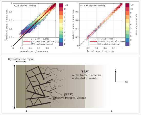
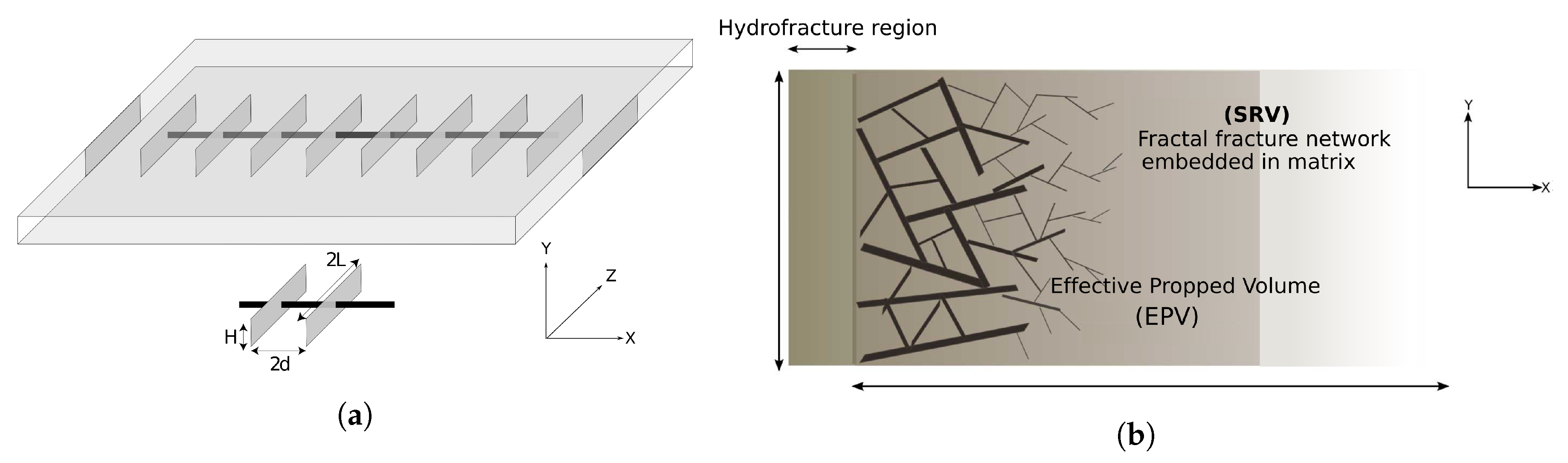
• SRV is composed of a fracture network and organic matrix.
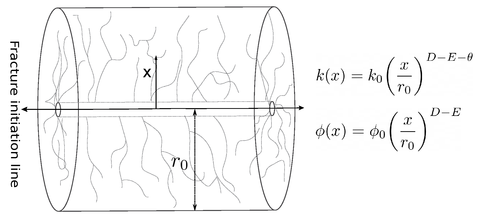
• SRV is nonuniform because of the power law distribution of properties of the fracture network.
• The single phase, compressible, and isothermal flow of gas is from right to left (see Figure 5b).
• The fracture permeability is 2–3 orders of magnitude higher than the matrix permeability.
• The matrix is disconnected from the hydrofracture and the wellbore, and only transfers gas into the fracture network.
• Gas flow from the fracture network is parallel to the hydrofracture plane (x-y plane).
• Depletion occurs only through the SRV, and the boundary flow is neglected.

Current practitioners of hydrofracturing might say that some of the parameters in Table 1 are not realistic for the wells completed today. For example, our $2d$ = 80–100 m. Currently, in most hydraulically fractured wells, $2d$ is around 10–30 m. We reply that the parameters in Table 1 are taken from the real well completion data. These data, purchased from DrillingInfo${}^{\copyright }$ (now Enverus), are from the older wells drilled with fewer stages in 2004, 2005, and 2006. Here, is the key point.

3. Results

We simulated 45 Barnett wells with the fractal SRV model to optimize the fracture permeability, $k_f$, and the microscale source term, s. Figure 6b shows the result of production history match of 45 wells, each with at least 13 years on production. These wells have maximum production rate in the beginning, starting from top right, and the production rate decreases with time for all the wells, making the points move left towards the origin with time. The scatter in the initial years is larger because of the undetermined flow rearrangements that die out with time. The width of the band between the two blue dotted lines in Figure 6b represents the 95% confidence interval that a new Barnett well with at least 13 years of production belongs to the same trend. One might think about this band as all the stochastic reservoir and well property fluctuations unaccounted for by our model. The optimized model parameters, $k_f$ and s, give important insights about the production mechanisms and pressure interactions in mudrocks at different scales.

3.1. Relation between the Optimized Parameters: Fracture Permeability $k_f$ and Microscale Source Terms

The second-order pressure diffusivity equation for the fracture and matrix is solved explicitly with the initial and boundary conditions given in Table 1. The unknown parameters in the simulations are the fracture permeability, $k_f$, the microscale source term, s, and the SRV volume. The best values of the unknown parameters are determined by numerical fitting of field production data with an optimization function.

Figure 7 shows the values of $k_f$ and s obtained from matching production histories of 45 wells. In general, a higher fracture permeability, $k_f$, gives a lower value of microscale source term, s. This happens because of the energy balance during hydrofracturing. A high $k_f$ results from the creation of dense macrofractures with better connectivity that consume a large amount of fracturing energy. In this case, a poorer connectivity at the microscale results and yields a smaller value of s. Therefore, there is an approximately hyperbolic relationship between these two parameters.

Different combinations of $k_f$ and s create different types of fracture networks after hydrofracturing. Figure 7 shows two extreme sets of wells encircled by the red and blue ellipses. For the red wells, the macroscale connectivity is high (high $k_f$) and the microscale connectivity is low (low s). For the blue wells, the macroscale connectivity is low (low $k_f)$ and the microscale connectivity is high (high s). These two sets of values define two different types of fracture systems that result in two distinct production profiles for the respective wells.

Figure 8 shows a schematic diagram of this concept. The black-bold vertical lines are a part of the macroscale discrete fracture network. The blue and red squares are the stimulated organic matrix and the dotted lines represent density of the microscale fractures draining gas from the organic matrix. Figure 8a represents the fracture system for the blue wells. It has poor macroscale connectivity (low $k_f$) and better microscale connectivity (high s because of high density of microfractures). Figure 8b represents the fracture system for the red wells. It has better macroscale connectivity (high $k_f$) and poorer microscale connectivity (low s because of low density of microfractures). A good or poor microscale connectivity represents permeability increase after hydrofracturing at the microscale. It does not represent the actual fracture area or new fracture surface created after hydrofracturing.

Figure 9 shows the effect of $k_f$ and s (particular fracture systems) on the production profiles of wells. Production decline of a well depends on the ratio $k_f/s$. This ratio represents the competing variables, $k_f$ and s, at the macroscale and microscale, and the extent of coupling between these two scales. This coupling defines stimulation effectiveness, and hence the fracture network in the SRV that controls the long-term production rate of a well. This coupling controls pressure communication between the macro- and microscale, i.e., the gas pressures in the fracture network and the organic matrix-hosting nanopores. The correct balance between pressure communication at these scales controls the overall cumulative production of wells. Two extreme cases of pressure coupling is represented by the stimulated system in Figure 8. In Figure 8a, fast pressure loss in the matrix supports fracture pressure. However, the low value of fracture permeability limits the cumulative production. In Figure 8b, a low value of s lowers pressure in the fracture network. However, high fracture permeability leads to higher cumulative production.

In Figure 9, the thicker curves represent higher values of $k_f/s$. At low values of $k_f/s$ (Figure 9a: blue curves), kerogen specks discharge gas at a higher rate because of better microscale connectivity. The low permeability of large-scale fractures is compensated by the high discharge rate from the kerogen specks and thus the initial production rate is very high. Kerogen exposed to the dense microfractures loses pressure more quickly, making production decline steeper. Cumulative production also decreases because of the loss of pressure support in the kerogen specks. Higher values of $k_f/s$ (Figure 9a: red curves) represent the opposite situation. Macroscale connectivity is good and microscale connectivity is poor. Slow discharge from the kerogen specks is compensated by better macroscale permeability that maintains ample production rate. The decline of production rate is gentler, because pressure support in the kerogen is maintained for a longer time. A slower decline of production rate leads to higher cumulative production. Thus, the idea is that the cumulative production depends on the ratio of $k_f/s$, because this ratio controls the pressure connectivity at different scale and governs the rate of its decrease and its magnitude over a period of time.

Other variables controlling production after a frac job are the volume of the stimulated reservoir, porosity, and gas saturation in the matrix. As evident in Figure 9b, cumulative production curves (the blue and red sets) do not become thicker monotonically with the increasing $k_f/s$. In particular, one of the blue curves has a low value of $k_f/s$, but still lies well above the red curves in the cumulative production and production rate plots. The reason is the initial mass in place, which is not constant in the production model and depends on the porosity of the system and the volume of rock we stimulate. The coupled effect of mass in place, stimulated volume and the ratio $k_f/s$ controls the overall production profile. Thus, permeability at the microscale and macroscale can give an idea about the production profile of a well. However, a better prediction of cumulative production requires a better understanding of matrix properties and of the stimulated volume after hydrofracturing.

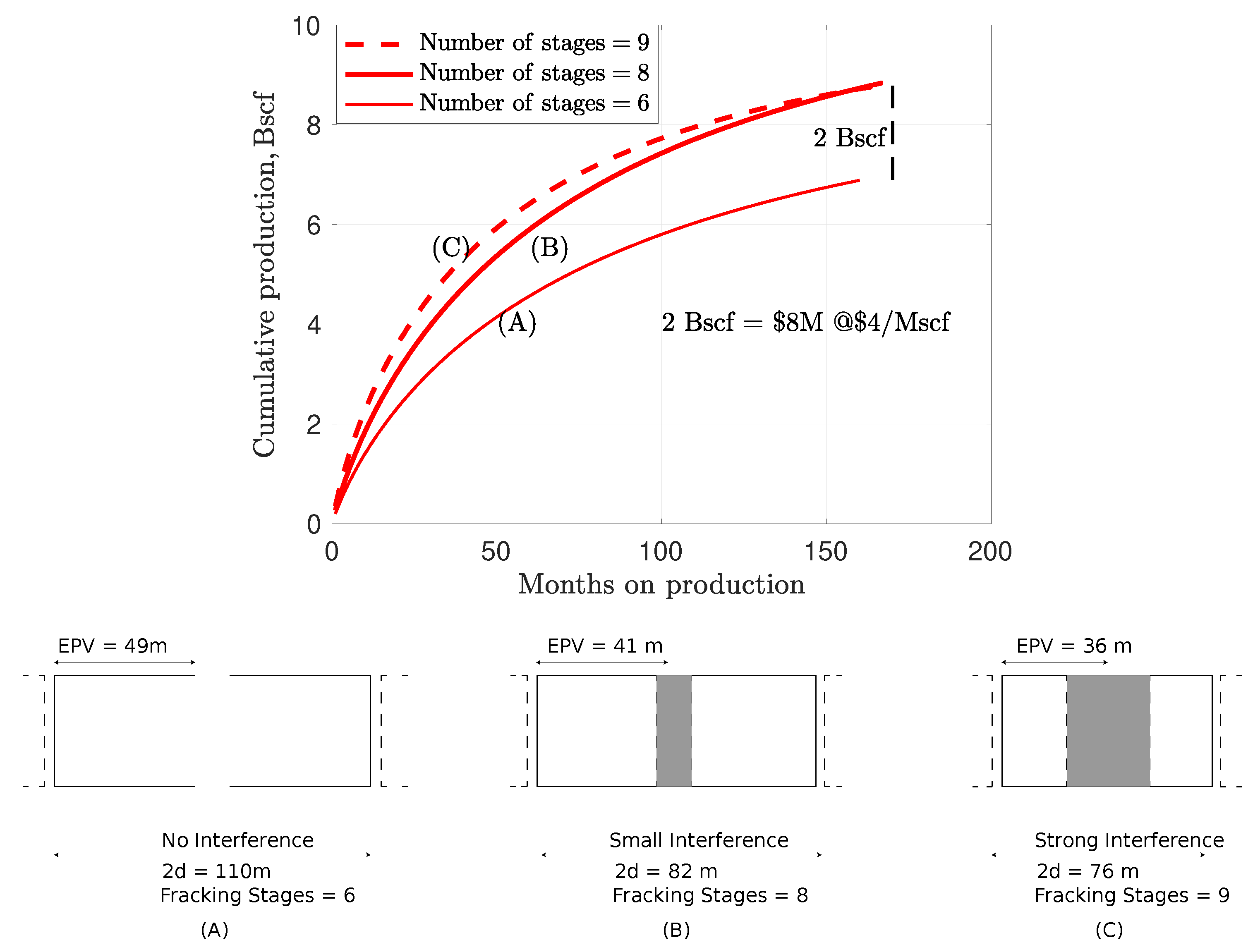
3.2. Effects of Interference and Distance between Frac Stages

Correct estimation of the extent of stimulated reservoir that defines the effectiveness of hydrofracturing is an important criterion in the design of efficient frac jobs. Figure 10, Curve A, shows the original cumulative production curve for a well. It is considered as the base case against which other simulation scenarios are compared. For the base case, the length of the well lateral is 660 m; the number of frac stages is 6; the hydrofractures spacing, $2d$, is 110 m; the width of stimulated volume (effective propped volume, EPV) from the numerical simulation is 49 m; and the cumulative production after 160 months is 7 Bscf.

Case 1: The number of frac stages is 8. For a fixed lateral length of a well, the width of effective stimulated volume (EPV) of each half of the stage is 41 m (660 m/($2\times$ number of frac stages)). Simulations show an increase of 2 Bscf in the cumulative production to 8.8 Bscf (see Figure 10, Curve B). Figure 10 (B) shows the schematic diagram of the system. When $2d$ decreases from 110 to 82 m, the width of EPV drops to 41 m. The overlap causes a weak interference between the stimulated volumes from both sides. Because the interference is weak, we assume negligible change in $k_f$ and s. Natural gas price of $4 per 1000 scf will generate an additional revenue of $8 million.

Case 2: For a fixed length of well lateral, 9 frac stages give $2d$ of 72 m and the EPV width of 36 m. A decrease in $2d$ results in a larger overlap area from the stimulation, resulting in strong interference (see Figure 10 (C)). We assume that the effect of strong interference on the flow properties is prominent at the microscale rather than at the macroscale. This interference increases the matrix-microscale fracture source term. Figure 10, Curve C, shows the simulated cumulative production with a $50\%$ higher source term, s, compared with the base case. The initial production rate increases, but the steeper decline in matrix pressure prevents cumulative production from increasing relative to eight hydrofracture stages. The limited improvement of EUR in response to denser hydrofracturing stages is also highlighted in recent work [57,58,59].

Nine hydrofracturing stages give the same cumulative production as eight stages with one major difference. With nine stages, the initial production rate is higher. This increased initial production rate calls for a trade off on the operator side. They may go with more frac stages and recover a major portion of their investment in the first few years of production, but handicap the well in the long run. Conversely, they may opt for an optimum number of stages and a lower production rate for a longer period of time and maximum profit. The latter option may not be available for the cash-strapped shale companies.

To design better frac jobs with optimum number of stages, correct estimation of EPV width using microseismic monitoring is a must to avoid interference. However, a better estimation of EPV does not guarantee a better production forecast. For the same EPV width inferred from the microsesimic data, cumulative production for individual wells can be different, depending on the fracture network developed by hydrofracturing. Figure 11 shows two wells of same lateral length (640 m), EPV width, hydrofracture height, and number of stages (5). The cumulative production varies by $13\%$ depending on the efficiency of the stimulated fracture network governed by the ratio $k_f/s$. This example highlights the importance of correct understanding of fracture network propagation during stimulation.

4. Materials and Methods

4.1. Diffusivity Equation in the SRV Matrix

The shale rock matrix inside of Stimulated Reservoir Volume (SRV) contains kerogen specks that host most of the nanopores. Gas in these nanopores is adsorbed as monolayers on the pore walls and fills the remainder of the pore volume as bulk fluid (free gas). The large specific surface area of shale pores has the potential to store a large amount of adsorbed gas. A decrease in pore pressure first produces free gas and later adsorbed gas as it gradually desorbs from the pore walls. Adsorbed gas layers decrease the effective radii of nanopores. True porosity, ${\varphi }_m$, is then replaced with effective porosity, ${\varphi }_{eff}$,60]. The general pressure diffusivity equation for a single phase compressible gas in a porous medium is given by:

$$\nabla ·\left({\rho }_g{u}_g\right)+\frac{\partial \left({\rho }_g{\varphi }_m\right)}{\partial t}+q=0$$

(4)

where q represents the flow interactions between matrix and fractures. Replacing ${\varphi }_m$ by ${\varphi }_{eff}$ and taking into account the effect of adsorbed gas, Equation (4) can be written as:

$$-\nabla ·\left({\rho }_g{u}_g\right)+q=\frac{\partial S_g{\rho }_g{\varphi }_{eff}}{\partial t}+\frac{\partial \left[{\rho }_a(1-{\varphi }_{eff})\right]}{\partial t}$$

(5)

where t is time, ${\rho }_g$ is the free gas density, ${\rho }_a$ is the adsorbed gas density per unit sample volume, ${\varphi }_{eff}$ is the effective porosity, and $u_g$ is the gas Darcy velocity. Using the following equations:

$$\begin{array}{cc}\hfill u_g& =-\frac{k_m}{{\mu }_g}\nabla p;c_g=\frac{1}{{\rho }_g}{\left(\frac{\partial {\rho }_g}{\partial p}\right)}_T;c_m=\frac{1}{{\varphi }_m}{\left(\frac{\partial {\varphi }_m}{\partial p}\right)}_T\hfill \\ \hfill c_{tot}& =c_g+c_m;K_a={\left(\frac{\partial {\rho }_a}{\partial {\rho }_g}\right)}_T=\frac{{\rho }_b{M}_g{V}_L{P}_L}{V_{sc}{\rho }_g{c}_g{(P_L+P_m)}^2},\hfill \end{array}$$

Equation (5) can be transformed into:

$$-\nabla ·\left({\rho }_g{u}_g\right)+q=-\frac{\partial }{\partial t}[S_g{\rho }_g{\varphi }_{eff}+{\rho }_a(1-{\varphi }_{eff})]$$

$$-\nabla ·\left({\rho }_g{u}_g\right)+q=-c_g{\rho }_g[S_g{\varphi }_{eff}+K_a(1-{\varphi }_{eff}]\frac{\partial p_m}{\partial t}$$

$$\frac{k_m}{{\mu }_g}\frac{{\partial }^2{p}_m}{\partial x^2}+q=-c_g{\rho }_g[S_g{\varphi }_{eff}+K_a(1-{\varphi }_{eff}]\frac{\partial p_m}{\partial t}$$

(6)

This is the pressure diffusion equation in the matrix of the stimulated region. As stated above, this matrix is in pseudo-steady state. We also assume that the mass transfer of gas from the matrix to the fractures depends only on the pressure difference between them. Neglecting the effect of adsorbed gas, and using ${\varphi }_{eff}={\varphi }_m$, gives the simplified version of Equation (6) as:

$$s{\left(\frac{x}{x_{HF}}\right)}^{D-2-\theta }\frac{k_m{\rho }_g}{{\mu }_g}(p_m-p_f)=-{\rho }_g{c}_g{\varphi }_m\frac{\partial p_m}{\partial t}$$

(7)

where the first term on the left is the gas transfer term from matrix and microfractures to macrofractures, $s{(x/w_{HF})}^{D-2-\theta }$ represents the shape factor controlling the magnitude of that transfer term, and its value depends on the distance from the hydrofracture. As we move away from the hydrofracture, a unit volume of the SRV matrix embodies fewer fractures. Fewer fractures mean a smaller surface area of contact between the matrix and fractures, and slower gas transfer between them.

4.2. Diffusivity Equation in SRV Fracture Network

Compared with the nanopores, fractures in the SRV have very wide apertures. As a result, all gas there is bulk. The general pressure diffusivity equation for a single phase compressible gas in a porous medium is given by:

$$\frac{\partial \left({\rho }_g{\varphi }_f\right)}{\partial t}+\nabla ·\left({\rho }_g{u}_g\right)+q=0$$

(8)

where q is the transfer term between matrix and fractures. Using the thermodynamic relation for compressibility and fluid velocity, Equation (8) can be written as:

$$\frac{\partial }{\partial x}\left[\frac{{\rho }_g{k}_f\left(x\right)}{{\mu }_g}\frac{\partial p_f}{\partial x}\right]+q=\frac{\partial }{\partial t}\left[{\rho }_g{\varphi }_f\left(x\right)\right]$$

(9)

Using the fractal relationships of fracture permeability and porosity from Equations (3) and (9) transforms into:

$$\frac{{\rho }_g{k}_f}{{\mu }_g}{\left[\frac{x}{w_{HF}}\right]}^{D-2-\theta }\left[\frac{{\partial }^2{p}_f}{\partial x^2}+\frac{D-2-\theta }{x}\frac{\partial p_f}{\partial x}\right]+q={\rho }_g{c}_g{\varphi }_f{\left(\frac{x}{w_{HF}}\right)}^{D-2}\frac{\partial p_f}{\partial t}$$

(10)

where ${\varphi }_f$ is the fracture porosity, $k_f$ is the fracture permeability, $p_f$ is the fracture pressure, D and $\theta$ are the fractal dimension and tortuosity index, and q is:

$$q=s{\left(\frac{x}{w_{HF}}\right)}^{D-2-\theta }\frac{k_m{\rho }_g}{{\mu }_g}(p_m-p_f)$$

The final pressure diffusivity equation is:

$$\frac{{\rho }_g{k}_f}{{\mu }_g}{\left[\frac{x}{w_{HF}}\right]}^{D-2-\theta }\left[\frac{{\partial }^2{p}_f}{\partial x^2}+\frac{D-2-\theta }{x}\frac{\partial p_f}{\partial x}\right]+s{\left(\frac{x}{w_{HF}}\right)}^{D-2-\theta }\frac{k_m{\rho }_g}{{\mu }_g}(p_m-p_f)={\rho }_g{c}_g{\varphi }_f{\left(\frac{x}{w_{HF}}\right)}^{D-2}\frac{\partial p_f}{\partial t}$$

(11)

4.3. Match of Production Data

Constraints on SRV Parameters

The matrix porosity ${\varphi }_m$, matrix permeability, $k_m$, height of the hydrofracture plane, H, and the tip-to-tip hydrofracture length L, are well characterized in the literature for the Barnett shale, as listed in Table 1. Before numerical simulation and parameter optimization, it is important to constrain some of the other basic parameters which define the SRV. These are the fractal dimension D, the volume and surface area of the generated fractures, and the width of the SRV effectively draining gas, i.e., $d_{EPV}$. Constraint on the volume and surface area of discrete fracture network: O’Malley et al. [61] presented a power law distribution of fracture length developed in a sheared shale sample. The volume and surface area of the generated fractures are given by:

$$\begin{array}{cc}\hfill & V={\int }_{R_0}^{R_1}dV\left(r\right)=\frac{N_0\varphi C_h(1-n)}{(7/2-n)(R_1^{1-n}-R_0^{1-n})}(R_1^{3.5-n}-R_0^{3.5-n})\hfill \\ \hfill & A={\int }_{R_0}^{R_1}dA\left(r\right)=\frac{2N_0\pi (1-n)}{(3-n)(R_1^{1-n}-R_0^{1-n})}(R_1^{3-n}-R_0^{3-n})\hfill \end{array}$$

(12)

where $R_0$ and $R_1$ are the minimum and maximum radii, respectively, of the penny-like fractures; $N_0$ is the total number of fractures; and n defines the size distribution of the fracture network. $C_h$ is a constant given by Adler et al. [62] as $C_h=5\times {10}^{-5}$ m${}^{1/2}$ (natural fractures) and $C_h=5\times {10}^{-4}$ m${}^{1/2}$ (hydraulically induced fractures).

A typical frac stage pumps around 750 m${}^3$ of water into the rock and $90\%$ of this water is retained in fractures. An average fracture aperture of 10 $\mathsf{\mu }$m creates surface area of the order of ${10}^7$ m${}^2$ to suck in the injected water. We assume that the fractures are circular in shape and exist in two groups: (a) small and reactivated natural fractures (radii: 1 mm–5 m); and (b) large fractures (radii: 5–50 m).

Large fractures create backbone of the discrete fracture network and small fractures define the microscale source term that interconnects the organic matrix and large fractures.

Out of the 750 m${}^3$ of injected water, $40\%$ (275 m${}^3$) flows into large fractures and $60\%$ flows into small fractures embedded in the matrix. The $40\%$ of the injected water in big fractures comes from the fact that each fracturing stage also takes up on average 250–300 m${}^3$ of proppant sand that keeps some fractures open (see Figure 12a. This sand may have an effective porosity of 0.3, and it displaces an additional 192 m${}^3$ of water into the small fractures.

Table 2. Comparison between small and large fracture parameters.

Parameters	Small Fractures	Large Fractures
$R_0$	1 mm	5 m
$R_1$	5 m	50 m
Volume	400 m${}^3$	275 m${}^3$
Area	$3\times {10}^7$ m${}^2$	$2.6\times {10}^5$ m${}^2$
Fractures	${10}^{13}$	360

shows the surface area created for small and large fractures using Equation (12). Surface area created by the small fractures is two orders of magnitude higher than that created by the large ones. This huge surface area of the small fractures is responsible for exposing nanopores in the organic material to the high permeability pathways. This surface area also connects the nanoscale organic pores and macroscale fractures. Total surface area created is of same order of magnitude as that expected from the average fracture aperture of $10\mathsf{\mu }$m. Surface area of same order was reported by Johri and Zoback [63] based on field fracture data and mechanical modeling.

Marder et al. [56] presented an analytical solution of fracture generation and simulated 2000 wells to show that the typical spacing between the large fracture planes should be 1–4 m to maintain production in mudrock. They argued that physically such a small fracture spacing may be impossible, but this distance can be considered as characteristic distance for the branching, complex fracture network. Raterman et al. [64] showed frequent occurrences of such macrofractures and permeability enhancement by discrete fractures in the Eagle Ford core samples (see Figure 12b. If we consider fracture planes spaced every 2 m ($L=180$ m and $H=30$ m), the fracture surface area we create is $4.3\times {10}^5$ m${}^2$. This surface area is of the same order of magnitude as that created by the large fractures in Table 1. Thus, large fractures numbering 300–400 create the backbone of the discrete fracture network and are consistent with the characteristic distance of 1–4 m between fracture planes.

Constraint on D: As shown in the above section, a portion of the injected water goes in macrofractures. The distribution of this water with distance from the hydrofracture face is used to constrain the value of D. The fractal dimension used in simulation is $D=1.8$. Figure 13a shows the strong effect of D on the injected water distribution. As we move from $D=1.7$ to $D=1.8$, the fracture porosity, ${\varphi }_{f_0}$ at the fracture face decreases from $1.8\%$ to $1.4\%$. For D = 1.7–1.8, 85–93% of the injected water is retained within $2d=85$ m, which is close to the average literature value of $2d$. However, $D=1.9$ decreases the fracture porosity, ${\varphi }_{f_0}$ to $0.1\%$ at the fracture face, thus making it an unreasonable choice for modeling. Such a low value of porosity at the fracture face is impossible. Expected porosity close to $1\%$ makes $D=1.8$ a good choice with $60\%$ of the water retained in the first few meters away from hydrofracture.

Constraint on the value of microscale source term, s, from the optimization function: The value of microscale source term, s, obtained after numerical fitting of production data is constrained with the power law distribution of total surface area created after hydrofracturing (see Table 2, total surface area). The continuous line in Figure 13 shows the power law distribution of the microscale source term, s (calculated from total surface area) for $D=1.8$. The values of s, obtained from simulation at the fracture face, cannot exceed the maximum value of the distribution at the fracture face. Values of s smaller than than the maximum value for the simulated wells reflect the fact that hydrofracturing is never $100\%$ efficient. For most wells, only a small part of the created surface area is well-connected and contributes to production.

5. Conclusions and Discussion

We simulated production histories of 45 Barnett wells using the concept of multiscale fractal reservoir. We showed that gas production from mudrocks depends on the quality of hydrofracturing job and reservoir properties. Here are our main conclusions:

• The classical ($\tau ,\mathcal{M}$) scaling of annual gas volumes produced from all non-refractured wells in the Barnett does an excellent job (see Figure 2), but the current ($k_f,s,D$) scaling gives deeper operational insights into well completion strategies (see Figure 6).
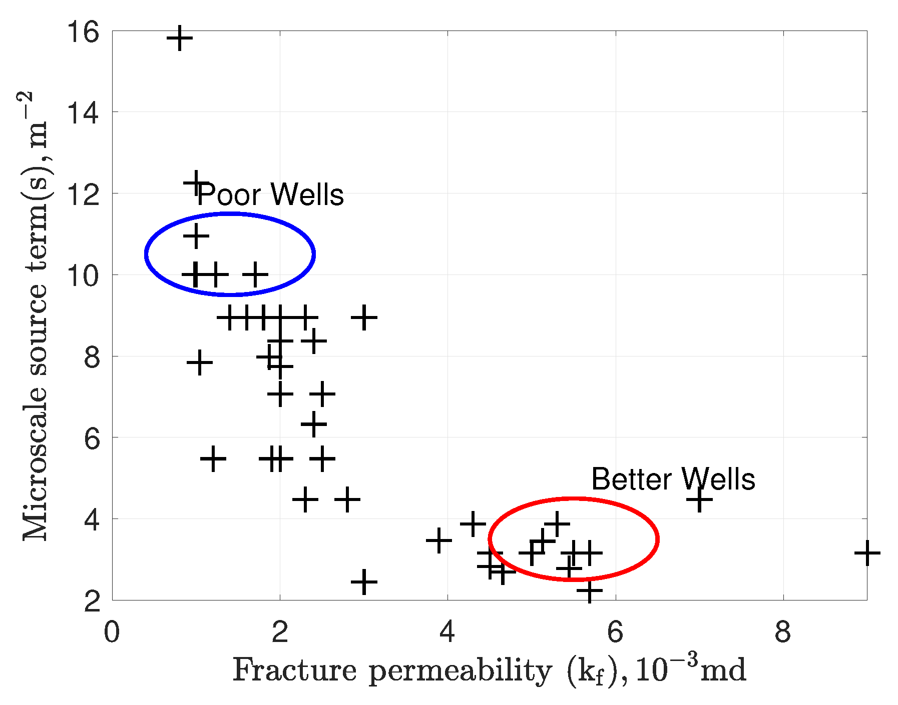
• The macroscale and microscale connectivities are represented by the fracture permeability, $k_f$, and the microscale source term, s. The higher the values of these two parameters are, the better flow connectivity at the respective scale is. In general, at higher fracture permeability, the microscale source term is lower, because of the balance of hydrofracturing energy (see Figure 7).
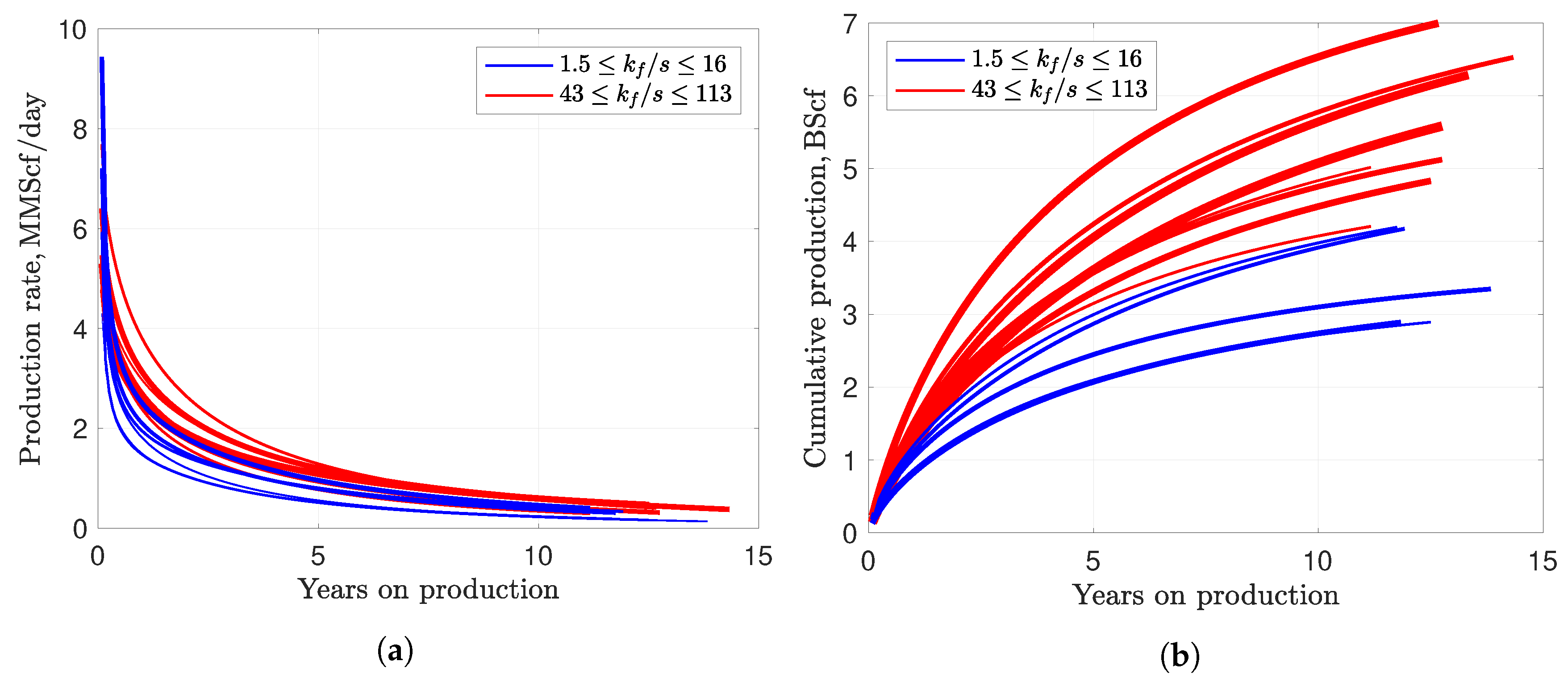
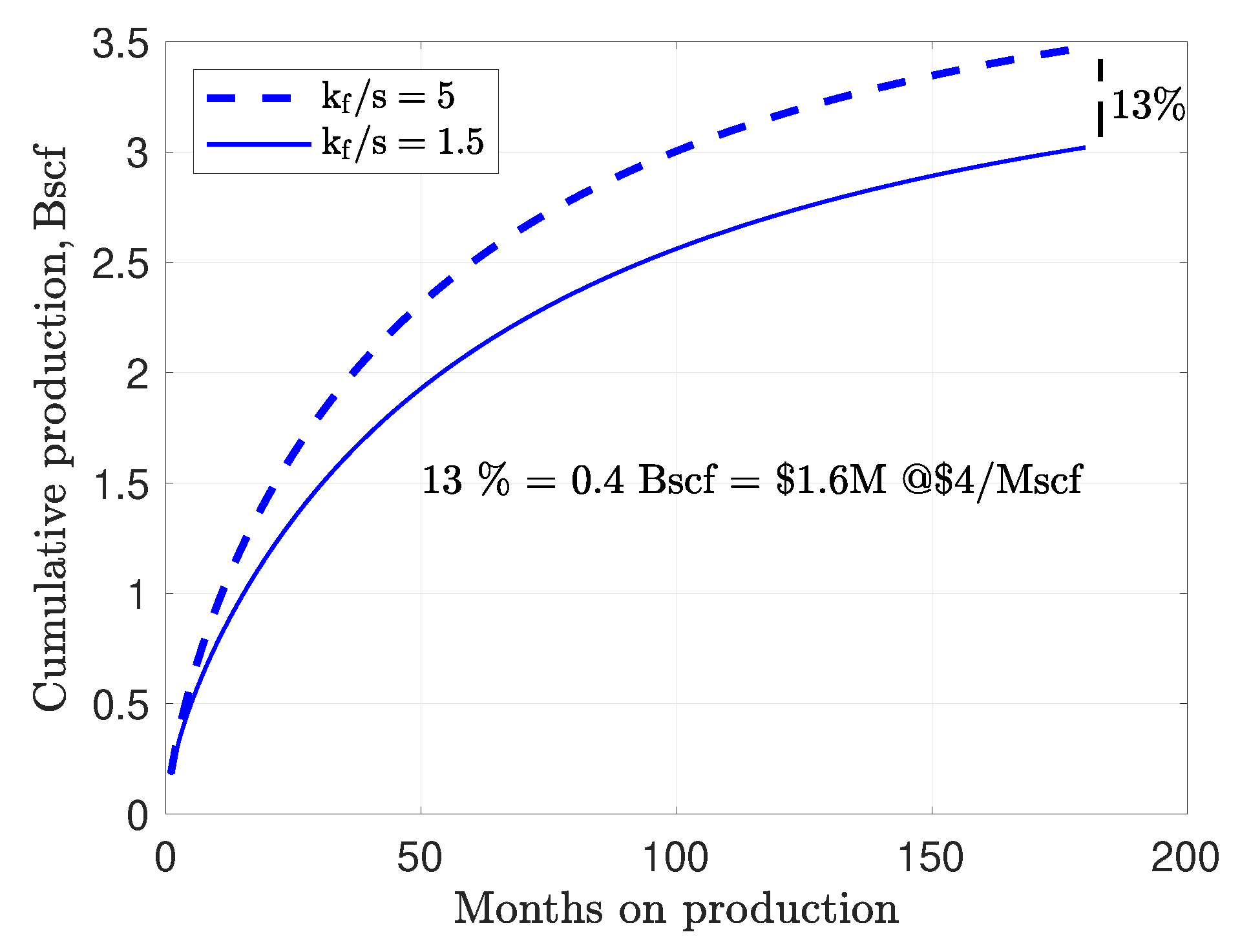
• The overall well quality depends on the ratio of macroscale and microscale connectivities, physically represented by the ratio $k_f/s$. A higher value of $k_f/s$ causes slow pressure decline in the matrix and results in high cumulative production. Poor microscale scale connectivity is compensated by better macroscale connectivity. A low value of $k_f/s$ causes high initial production rate resulting from fast gas discharge at the microscale. The matrix pressure depletes faster and limits overall cumulative production.
• There can be indirect ways of accessing the ratio of $k_f/s$ using the magnitude of microseismic events during hydrofracturing. The distribution of event magnitudes can be used to estimate the size distribution of microfractures/macrofractures created in the source rock. Eventually, hydrofracturing can be optimized by interpreting microseismicity.
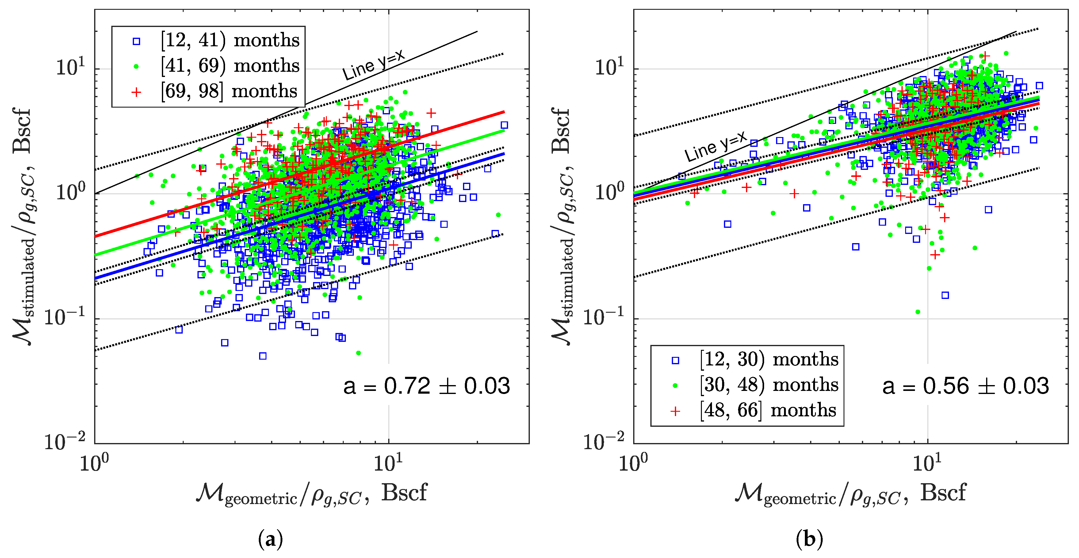
• Stimulated mass is an important factor in controlling the overall production. The non-monotonic increase in the cumulative production histories for the 13 Barnett wells in Figure 9 highlights the importance of initial mass in place, which is the product of gas density, porosity, gas saturation, and volume stimulated after hydrofracturing.
• Efficient hydrofracturing is crucial to maximizing production. An important factor is the average distance between hydrofractures, $2d$. Small values of $2d$ can cause strong interference between two consecutive hydrofractures and can accelerate pressure loss in the matrix, thus limiting cumulative production (see Figure 10). Another key factor is the correct estimation of the Effective Propped Volume (EPV) width using microseismic data. The EPV width can give an estimate for the number of hydrofractures one should generate without causing a strong pressure interference and decreasing production.
• In addition to the correct estimation of EPV width from a cloud of microseismic events, it is important to understand configuration of the new/reactivated fracture network after stimulation. The same EPV width can give different EURs, depending on the ratio of $k_f/s$ that controls the efficiency of the backbone fracture network that drains gas at different scales (see Figure 9).

This paper provides a quantitative understanding of multiscale connectivity among the nanopores, microfractures, and the hydrofracture crack network in mudrocks (shales). The most influential reservoir parameters are the fracture network permeability and the microscale source term connecting the fracture systems at two different scales. Stimulation enhances fracture flow capacity by activating the existing natural fractures and increases the organic matrix contact area by cracking the rock. The microfractures bridge gaps between the isolated nanopores and the stimulated fracture network. Together they form a complex fracture network, through which shale gas migrates from the nanopores, all the way up to the well laterals. These multiscale properties of gas flow imply that reservoir characterization is quite important in the evaluation of shale gas production. In addition, a good quality shale matrix can yield high production only with successful stimulation. Instead of drilling longer horizontal wells to increase production, the goal should be a more effective rock stimulation by designing better hydrofracturing jobs with the help of microseismic data.

Although the model presented here provides good quantitative and qualitative insights about the production mechanisms, it can be improved. Incorporation of the effects of multiphase flow, boundary flow, diffusion, decrease of reservoir permeability under compaction, and reopening of fractures could lead to an even more robust production model.

References

1. Patzek, T.W.; Male, F.; Marder, M. Gas production in the Barnett shale obeys a simple scaling theory. Proc. Natl. Acad. Sci. USA 2013, 110, 19731–19736. [Google Scholar] [CrossRef] [Green Version]
2. Patzek, T.W.; Male, F.; Marder, M. A simple model of gas production from hydrofractured horizontal wells in shales. AAPG Bull. 2014, 98, 2507–2529. [Google Scholar] [CrossRef]
3. Patzek, T.W.; Saputra, W.; Kirati, W.; Marder, M. Generalized Extreme Value Statistics, Physical Scaling, and Forecasts of Gas Production in the Barnett Shale. Energy Fuels 2019, 33, 12154–12169. [Google Scholar] [CrossRef]
4. Anonymous. Report Forecasts “Major Slowdown” in US Oil Output Growth. J. Pet. Technol. 2019. Available online: https://pubs.spe.org/en/jpt/jpt-article-detail/?art=6197 (accessed on 5 April 2020).
5. Suk Min, K.; Sen, V.; Ji, L.; Sullivan, R.B. URTeC: 2897656: Optimization of Completion and Well Spacing for Development of Multi-Stacked Reservoirs using Integration of Data Analytics, Geomechanics and Reservoir Flow Modeling. In Proceedings of the SPE/AAPG/SEG Unconventional Resources Technology Conference, Houston, TX, USA, 23–25 July 2018; Society of Petroleum Engineers: Richardson, TX, USA, 2018; pp. 1–11. [Google Scholar]
6. Tugan, M.F.; Weijermars, R. Improved EUR prediction for multi-fractured hydrocarbon wells based on 3-segment DCA: Implications for production forecasting of parent and child wells. J. Pet. Sci. Eng. 2020, 187, 106692. [Google Scholar] [CrossRef]
7. Patzek, T.W. Barnett Shale in Texas: Promise and Problems. In Proceedings of the Seminar at the Bureau of Economic Geology, UT Austin, Austin, TX, USA, 26 May 2019. [Google Scholar] [CrossRef]
8. Eftekhari, B.; Marder, M.; Patzek, T.W. Field data provide estimates of effective permeability, fracture spacing, well drainage area and incremental production in gas shales. J. Nat. Gas Sci. Eng. 2018, 56, 141–151. [Google Scholar] [CrossRef]
9. Patzek, T.W. SPE 24040: Surveillance of South Belridge Diatomite. In Proceedings of the Western Regional SPE Meeting, Bakersfield, CA, USA, 30 March–1 April 1992. [Google Scholar] [CrossRef]
10. Patzek, T.W.; Wardana, S.; Kirati, W. SPE187226-MS: A Simple Physics-Based Model Predicts Oil Production from Thousands of Horizontal Wells in Shales. In Proceedings of the SPE Annual Technical Conference and Exhibition, San Antonio, TX, USA, 9–11 October 2017. [Google Scholar] [CrossRef] [Green Version]
11. Saputra, W.; Kirati, W.; Patzek, T.W. Generalized Extreme Value Statistics, Physical Scaling and Forecasts of Oil Production in the Bakken Shale. Energies 2019, 12, 3641. [Google Scholar] [CrossRef] [Green Version]
12. Saputra, W.; Kirati, W.; Patzek, T.W. Physical scaling of oil production rates and ultimate recovery from all horizontal wells in the Bakken shale. Energies 2020, 13, 2052. [Google Scholar] [CrossRef] [Green Version]
13. Tarek, A. Reservoir Engineering Handbook, 4th ed.; Gulf Professional Publishing: Oxford, UK, 2010. [Google Scholar]
14. Kenomore, M.; Hassan, M.; Malakooti, R.; Dhakal, H.; Shah, A. Shale gas production decline trend over time in the Barnett Shale. J. Pet. Sci. Eng. 2018, 165, 691–710. [Google Scholar] [CrossRef] [Green Version]
15. Arps, J.J. Analysis of decline curves. Trans. AIME 1945, 160, 228–247. [Google Scholar] [CrossRef]
16. Bailey, D. Decline Rate in Fractured Gas Wells. OGJ 1982, 117–118. [Google Scholar]
17. Muralidharan, V.; Joshi, K. Myths and Facts of Forecasting Horizontal Well Production in Unconventional Reservoirs—Are We Complicating a Simple Analysis? In Proceedings of the 6th Unconventional Resources Technology Conference, Houston, TX, USA, 23–25 July 2018; American Association of Petroleum Geologists: Tulsa, OK, USA, 2018. [Google Scholar]
18. Aybar, U.; Eshkalak, M.O.; Sepehrnoori, K.; Patzek, T.W. The effect of natural fractures closure on long-term gas production from unconventional resources. J. Nat. Gas Sci. Eng. 2014, 21, 1205–1213. [Google Scholar] [CrossRef]
19. Aybar, U.; Yu, W.; Eshkalak, M.O.; Sepehrnoori, K.; Patzek, T. Evaluation of production losses from unconventional shale reservoirs. J. Nat. Gas Sci. Eng. 2015, 23, 509–516. [Google Scholar] [CrossRef]
20. Weijermars, R.; Nandlal, K.; Khanal, A.; Tugan, M.F. Comparison of pressure front with tracer front advance and principal flow regimes in hydraulically fractured wells in unconventional reservoirs. J. Pet. Sci. Eng. 2019, 183, 106407. [Google Scholar] [CrossRef]
21. Loucks, R.G.; Reed, R.M.; Ruppel, S.; Hammes, U. Preliminary Classification of Matrix Pores in Mudrocks; The Gulf Coast Association of Geological Societies: New Orleans, LA, USA, 2010. [Google Scholar]
22. Curtis, M.E.; Ambrose, R.J.; Sondergeld, C.H. Structural characterization of gas shales on the micro-and nano-scales. In Proceedings of the Canadian Unconventional Resources and International Petroleum Conference, Calgary, AB, Canada, 19–21 October 2010; Society of Petroleum Engineers: Richardson, TX, USA, 2010. [Google Scholar]
23. Nelson, P.H. Pore-throat sizes in sandstones, tight sandstones, and shales. AAPG Bull. 2009, 93, 329–340. [Google Scholar] [CrossRef]
24. Sakhaee-Pour, A.; Bryant, S.L. Gas permeability of shale. SPE Reserv. Eval. Eng. 2012, 15, 401–409. [Google Scholar] [CrossRef]
25. Sondergeld, C.H.; Ambrose, R.J.; Rai, C.S.; Moncrieff, J. Micro-structural studies of gas shales. In Proceedings of the SPE Unconventional Gas Conference, Pittsburgh, PA, USA, 23–25 February 2010; Society of Petroleum Engineers: Richardson, TX, USA, 2010. [Google Scholar]
26. Tian, H.; Pana, L.; Xiao, X.; Wilkins, R.W.T.; Meng, Z.; Huangd, B. A preliminary study on the pore characterization of Lower Silurian black shales in the Chuandong Thrust Fold Belt, southwestern China using low pressure N2 adsorption and FE-SEM methods. Mar. Pet. Geol. 2013, 48, 8–19. [Google Scholar] [CrossRef]
27. Slatt, R.M.; O′Brien, N.R. Pore types in the Barnett and Woodford gas shales: Contribution to understanding gas storage and migration pathways in fine-grained rocks. AAPG Bull. 2011, 95, 2017–2030. [Google Scholar] [CrossRef]
28. Huang, Z.; Chen, J.; Xue, H.; Wang, Y.; Wang, M.; Deng, C. Microstructural characteristics of the cretaceous Qingshankou formation shale, Songliao basin. Pet. Explor. Dev. 2013, 40, 61–68. [Google Scholar] [CrossRef]
29. Berthonneau, J.; Obliger, A.; Valdenaire, P.L.; Grauby, O.; Ferry, D.; Chaudanson, D.; Levitz, P.; Kim, J.J.; Ulm, F.J.; Pellenq, R.J.M. Mesoscale structure, mechanics, and transport properties of source rocks’ organic pore networks. Proc. Natl. Acad. Sci. USA 2018, 115, 12365–12370. [Google Scholar] [CrossRef] [PubMed] [Green Version]
30. Anderson, D.M.; Nobakht, M.; Moghadam, S.; Mattar, L. Analysis of production data from fractured shale gas wells. In Proceedings of the SPE Unconventional Gas Conference, Pittsburgh, PA, USA, 23–25 February 2010; Society of Petroleum Engineers: Richardson, TX, USA, 2010. [Google Scholar]
31. Fan, D. A Hybrid Transient Flow Model for Performance Evaluation of Shale Gas Reservoirs. Ph.D. Thesis, Department of Petroleum Engineering, Texas Tech University, Lubbock, TX, USA, 2015. [Google Scholar]
32. Stalgorova, E.; Mattar, L. Practical analytical model to simulate production of horizontal wells with branch fractures. In Proceedings of the SPE Canadian Unconventional Resources Conference, Calgary, AB, Canada, 30 October–1 November 2012; Society of Petroleum Engineers: Richardson, TX, USA, 2012. [Google Scholar]
33. Fan, D.; Ettehadtavakkol, A. Transient shale gas flow model. J. Nat. Gas Sci. Eng. 2016, 33, 1353–1363. [Google Scholar] [CrossRef]
34. Yuan, B.; Zheng, D.; Moghanloo, R.G.; Wang, K. A novel integrated workflow for evaluation, optimization, and production predication in shale plays. Int. J. Coal Geol. 2017, 180, 18–28. [Google Scholar] [CrossRef]
35. Darishchev, A.; Lemouzy, P.; Rouvroy, P. On simulation of flow in tight and shale gas reservoirs. In Proceedings of the SPE Unconventional Gas Conference and Exhibition, Muscat, Oman, 28–30 January 2013; Society of Petroleum Engineers: Richardson, TX, USA, 2013. [Google Scholar]
36. Zheng, D.; Yuan, B.; Moghanloo, R.G. Analytical modeling dynamic drainage volume for transient flow towards multi-stage fractured wells in composite shale reservoirs. J. Pet. Sci. Eng. 2017, 149, 756–764. [Google Scholar] [CrossRef]
37. Zheng, D.; Moghanloo, R.G.; Yuan, B.; Dong, X. Modeling dynamic drainage volume for multi-stage fractured wells in composite shale systems: New analytical solution for transient linear flow. In Proceedings of the SPE Asia Pacific Hydraulic Fracturing Conference, Beijing, China, 24–26 August 2016; Society of Petroleum Engineers: Richardson, TX, USA, 2016. [Google Scholar]
38. Chang, J.; Yortsos, Y.C. Pressure transient analysis of fractal reservoirs. SPE Form. Eval. 1990, 5, 31–38. [Google Scholar] [CrossRef]
39. Acuna, J.A.; Ershaghi, I.; Yortsos, Y.C. Practical application of fractal pressure transient analysis of naturally fractured reservoirs. SPE Form. Eval. 1995, 10, 173–179. [Google Scholar] [CrossRef]
40. O Shaughnessy, B.; Procaccia, I. Diffusion on fractals. Phys. Rev. A 1985, 32, 3073. [Google Scholar] [CrossRef]
41. Havlin, S.; Ben-Avraham, D. Diffusion in disordered media. Adv. Phys. 1987, 36, 695–798. [Google Scholar] [CrossRef]
42. Olarewaju, J. Modeling fractured reservoirs with stochastic fractals. In Proceedings of the Abu Dhabi International Petroleum Exhibition and Conference, Abu Dhabi, UAE, 13–16 October 1996; Society of Petroleum Engineers: Richardson, TX, USA, 1996. [Google Scholar]
43. Chang, J.; Yortsos, Y.C. A note on pressure-transient analysis of fractal reservoirs. SPE Adv. Technol. Ser. 1993, 1, 170–171. [Google Scholar] [CrossRef]
44. Chakrabarty, C.; Tortike, W.S.; Ali, S.M.F. Complexities in the Analysis of Pressure-Transient Response for Non-Newtonian power-law fluid flow in fractal Reservoirs. In Proceedings of the SPE Eastern Regional Meeting, Pittsburgh, PA, USA, 2–4 November 1993; Society of Petroleum Engineers: Richardson, TX, USA, 1993. [Google Scholar]
45. Chakrabarty, C.; Tortike, W.S.; Ali, S.M.F. Transient Flow Behaviour Of Non-Newtonian Power-Law Fluids In Fractal Reservoirs. In Proceedings of the Annual Technical Meeting, Calgary, AB, Canada, 9–12 May 1993; Petroleum Society of Canada: Calgary, AB, Canada, 1993. [Google Scholar]
46. Beier, R.A. Pressure transient field data showing fractal reservoir structure. In Proceedings of the CIM/SPE International Technical Meeting, Calgary, AB, Canada, 10–13 June 1990; Petroleum Society of Canada: Calgary, AB, Canada, 1990. [Google Scholar]
47. Flamenco-Lopez, F.; Camacho-Velazquez, R. Determination of fractal parameters of fracture networks using pressure-transient data. SPE Reserv. Eval. Eng. 2003, 6, 39–47. [Google Scholar] [CrossRef]
48. Camacho-Velazquez, R.; Fuentes-Cruz, G.; Vasquez-Cruz, M.A. Decline curve analysis of fractured reservoirs with fractal geometry. In Proceedings of the International Oil Conference and Exhibition in Mexico, Cancun, Mexico, 31 August–2 September 2006; Society of Petroleum Engineers: Richardson, TX, USA, 2006. [Google Scholar]
49. Camacho-Velazquez, R.; Vasquez-Cruz, M.A.; Castrejon-Aivar, A.; Arana-Ortiz, V. Pressure transient and decline curve behaviors in naturally fractured vuggy carbonate reservoirs. In Proceedings of the SPE Annual Technical Conference and Exhibition, San Antonio, TX, USA, 29 September–2 October 2002; Society of Petroleum Engineers: Richardson, TX, USA, 2002. [Google Scholar]
50. Fuentes-Cruz, G.; Camacho-Velazquez, R.; Vasquez-Cruz, M.A. A Unified Approach for Falloff and Buildup Tests Analysis Following a Short Injection/Production Time. In Proceedings of the SPE Western Regional Meeting, Anaheim, CA, USA, 27–29 May 2010; Society of Petroleum Engineers: Richardson, TX, USA, 2010. [Google Scholar]
51. Cossio Santizo, M. A Semi-Analytic Solution for Flow in Finite-Conductivity Vertical Fractures Using Fractal Theory. Master’s Thesis, Texas A&M University, College Station, TX, USA, 2012. [Google Scholar]
52. Cossio, M.; Moridis, G.; Blasingame, T.A. A Semianalytic Solution for Flow in Finite-Conductivity Vertical Fractures by Use of Fractal Theory. SPE J. 2013, 18, 83–96. [Google Scholar] [CrossRef]
53. Wang, W.; Shahvali, M.; Su, Y. A semi-analytical fractal model for production from tight oil reservoirs with hydraulically fractured horizontal wells. Fuel 2015, 158, 612–618. [Google Scholar] [CrossRef]
54. Fan, D.; Ettehadtavakkol, A. Semi-analytical modeling of shale gas flow through fractal induced fracture networks with microseismic data. Fuel 2017, 193, 444–459. [Google Scholar] [CrossRef]
55. Wang, W.; Su, Y.; Sheng, G.; Cossio, M.; Shang, Y. A mathematical model considering complex fractures and fractal flow for pressure transient analysis of fractured horizontal wells in unconventional reservoirs. J. Nat. Gas Sci. Eng. 2015, 23, 139–147. [Google Scholar] [CrossRef]
56. Marder, M.; Chen, C.H.; Patzek, T. Simple models of the hydrofracture process. Phys. Rev. E 2015, 92, 062408. [Google Scholar] [CrossRef] [Green Version]
57. Khanal, A.; Weijermars, R. Pressure depletion and drained rock volume near hydraulically fractured parent and child wells. J. Pet. Sci. Eng. 2019, 172, 607–626. [Google Scholar] [CrossRef]
58. Weijermars, R.; Khanal, A. Production Interference of Hydraulically Fractured Hydrocarbon Wells: New Tools for Optimization of Productivity and Economic Performance of Parent and Child Wells. In Proceedings of the SPE Europec featured at 81st EAGE Conference and Exhibition, London, UK, 3–6 June 2019; Society of Petroleum Engineers: Richardson, TX, USA, 2019. [Google Scholar]
59. Weijermars, R.; van Harmelen, A.; Zuo, L. Flow interference between frac clusters (Part 2): Field example from the Midland basin (Wolfcamp formation, Spraberry trend field) with implications for hydraulic fracture design. In Proceedings of the Unconventional Resources Technology Conference, Austin, TX, USA, 24–26 July 2017; Society of Exploration Geophysicists: Tulsa, OK, USA; American Association of Petroleum Geologists: Tulsa, OK, USA, 2017; pp. 989–1004. [Google Scholar]
60. Pang, Y.; Soliman, M.Y.; Deng, H.; Emadi, H. Analysis of effective porosity and effective permeability in shale-gas reservoirs with consideration of gas adsorption and stress effects. SPE J. 2017, 22, 1–12. [Google Scholar] [CrossRef]
61. O’Malley, D.; Karra, S.; Currier, R.P.; Makedonska, N.; Hyman, J.D.; Viswanathan, H.S. Where does water go during hydraulic fracturing? Groundwater 2016, 54, 488–497. [Google Scholar] [CrossRef]
62. Adler, P.M.; Thovert, J.-F.; Mourzenko, V.V. Fractured Porous Media; Oxford University Press: Oxford, UK, 2013. [Google Scholar]
63. Johri, M.; Zoback, M.D. The evolution of stimulated reservoir volume during hydraulic stimulation of shale gas formations. In Proceedings of the Unconventional Resources Technology Conference, Denver, CO, USA, 12–14 August 2013; Society of Exploration Geophysicists: Tulsa, OK, USA; American Association of Petroleum Geologists: Tulsa, OK, USA, 2013; pp. 1661–1671. [Google Scholar]
64. Raterman, K.T.; Farrell, H.E.; Mora, O.S.; Janssen, A.L.; Gomez, G.A.; Busetti, S.; McEwen, J.; Friehauf, K.; Rutherford, J.; Reid, R.; et al. Sampling a Stimulated Rock Volume: An Eagle Ford Example. In Proceedings of the SPE Conference. Unconventional Resources Technology Conference (URTEC), Austin, TX, USA, 24–26 July 2017. [Google Scholar]
Figure 1. In conventional reservoirs, ultimate recovery factor for a well (the ratio of gas produced from the stimulated reservoir volume (SRV), M stimulated , to the original gas in place in the reservoir compartment assigned to a well, M geometric ) is proportional to the compartment size. This is not so in mudrock reservoirs, where produced gas is only partially connected to the reservoir compartment. In this case, produced gas volume is proportional to the compartment size raised to a fractional (fractal) power exponent a < 1 . The weaker is the mudrock connectivity, the smaller is the exponent. (a) The power law scaling for three intervals of times on production (three age groups) of Barnett shale wells with the ages shown in the legend. The three solid lines are the result of a joint linear regression of production from these three groups of wells. The 95% CI that the regression explains the linear trend in the blue data points are drawn as the dotted lines above and below the blue fit. The 95% CI that a new well will belong to the blue dataset is shown as the outer dotted lines. The single power law exponent a = 0.72 explains all data. (b) The corresponding three linear trends for Haynesville almost overlay one another. Most of the poorest producers are on the Texas side of the play. Notice that the power exponent explaining gas production from the Haynesville wells a = 0.56 is smaller than that in Barnett. Hence, on average, SRV connectivity in Haynesville is weaker than that in Barnett. Source: The unpublished calculations for [1,2]. The Haynesville play productivity will be addressed in a separate paper.
Energies 13 02348 g001
Figure 2. (a) Up to fifteen years on production from 11,312 non-refractured wells in the Barnett were matched with hyperbolic DCA between January 1998 and December 2019. For each well, we normalize the predicted cumulative gas production with the last recorded value of cumulative production (max cum.) and plot it versus the normalized actual cumulative production. The increasingly hotter colors code the elapsed years on production from 1 to ≥11 years. Ideally, the annual cumulative production dots would track the black dashed diagonal ( x = y actual = predicted ). In contrast, the least squares fit of our hyperbolic DCA calculations is offset above the diagonal and is biased, overestimating EUR. The 95% confidence interval (CI) that a new well will belong to this dataset is plotted as the blue dotted lines. (b) The same wells matched with an extension of the scaling in [3]. Consecutive hydrofractures in 4877 of these wells pressure-interfere with one another. There are 96,548 dots colored by each year on production, i.e., on average 8.2 years on production are plotted for each well. Time on production progresses along the diagonal away from the origin. The least squares fit of this cross-plot has less bias and offset compared with the hyperbolic DCA on the left. The 95% CI that a new well will belong to this dataset is plotted as the two red dotted lines. The red CI band on the right is narrower than the blue band on the left. In addition, the two color distributions are quite different. We conclude that the predicted annual production volumes from both the non-interfering and exponentially declining Barnett wells are accurate.
Energies 13 02348 g002
Figure 3. Probability distribution functions for the parameters of the hyperbolic DCA matches of 11,312 non-refractured wells in the Barnett plotted in Figure 2a. For each well, we apply the algorithm from the Reservoir Engineering Handbook (4 th edition) [13] to solve for the Arp’s decline-curve exponent, b, and the initial decline rate, D i . The mean values of b and D i are 1.31 and 0.35 month 1 , respectively. In comparison, a recent published DCA analysis for 10,237 Barnett wells [14] gives the average values of b and D i as 1.477 and 0.1362 month 1 , respectively. Even though the original formulation of hyperbolic DCA by Arps [15] requires b [ 0 , 1 ] , for many hydrofractured gas wells, b > 1 , and sometimes b is as high as 3.5 [16]. Therefore, we did not constrain the b exponents in Figure 2. Constraining them can result in the unrealistic shapes of decline curves that deviate from production rates observed over finite time intervals [17].
Energies 13 02348 g003
Figure 4. The fractures, represented by the dotted lines, initiate at the center of the cylinder and follow a branching pattern, spreading through the rock. Away from the center, density of the branched fractures decreases following a power law, as do the fracture porosity, ϕ , and fracture permeability, k. In the equation, D is the fractal dimension, E is the Euclidean dimension ( E = 1 for one fracture; E = 2 for more fractures), and θ is the tortuosity index of the fracture network. Adapted from [38].
Energies 13 02348 g004
Figure 5. (a) A horizontal well with eight hydrofracture stages. The hydrofractures are perpendicular to the wellbore and gas flows into each hydrofracture from both sides. The hydrofracture permeability is infinite relative to the stimulated matrix. Adapted from [56]. (b) Planar view of half-SRV after hydrofracturing. The branching fracture network starts at the fracture face and its density decreases away from it. This fracture network interacts with the organic matrix and drains gas into the hydrofracture. The fracture porosity, ϕ f , and permeability, k f , also decrease as we move away from the fracture face. The Effective Propped Volume (EPV) is defined by the distance d E P V up to which the fractures are connected well enough to drain gas from the local organic matrix.
Energies 13 02348 g005
Figure 6. (a) Predicted vs. actual annual cumulative gas production from 4877 pressure-interfering wells in the Barnett play scaled with an extension of the method in [1]. There are 37,942 dots, i.e., on average 7.6 years on production are plotted for each well (see the caption of Figure 2). The least squares fit of this cross-plot has some bias and offset ( predicted = 0.92 actual + 0.07 ), which is not surprising for such a large heterogeneous set of wells. (b) The multiscale (“ k f , s , D ”) well performance model proposed in this paper. We plot the predicted cumulative gas production in one year increments vs. the one measured in 45 horizontal wells in the Barnett, each with 13.3 years on production on average, and each pressure-interfering. There are 597 dots of 11 colors. Time is progressing along the diagonal away from the origin. The least squares fit of this cross-plot has no bias and offset ( predicted = 0.99 actual + 0.01 ). The 95% CI that this fit explains the linear trend in data is so tight we do not plot it. The 95% CI that a new well will belong to this dataset is plotted as the two red dotted lines. A mixture of simple scaling models published elsewhere and this paper’s multiscale model can provide crucial economic insights about well completions.
Energies 13 02348 g006
Figure 7. The microscale source term, s, represents microscale connectivity and the fracture permeability, k f , represents macroscale connectivity for 45 Barnett wells. There is a tradeoff between the macroscale and microscale stimulation because of energy conservation. More energy spent on the macroscale stimulation leaves less energy available for the microscale stimulation. The result is higher values of k f and lower values of s, and vice versa. The extreme values in the red and blue ellipse represent two different types of fracture networks after hydrofracturing that result in two different types of production profiles.
Energies 13 02348 g007
Figure 8. (a) Stimulated rock with low k f and high s. Density of the discrete macroscale fracture network is low and density of the microscale fractures (dotted lines) in the organic matrix is high. This situation results in a faster pressure decline in the organic matrix. Low permeability at the macroscale is compensated by higher permeability at the microscale. (b) Stimulated rock with high k f and low s. Density of the discrete macroscale fracture network is high and density of microscale fractures (dotted lines) in the organic matrix is low, causing a slower pressure decline in the organic matrix. Low permeability at the microscale is compensated by higher permeability at the macroscale.
Energies 13 02348 g008
Figure 9. Gas production rate (a) and cumulative production (b) depend on the ratio k f / s . The thickness of each line increases with the increasing k f / s . This ratio represents the contributions from the macroscale and microscale discharge processes. For the low values of this ratio, initial production rate can be very high with a steep production decline (blue curves). Faster production decline caused by the low k f / s gives lower ultimate cumulative production. The two sets of curves do not increase monotonically with k f / s , because of uncertainty in the initial mass in place, which depends on the porosity, gas saturation and the stimulated volume after hydrofracturing.
Energies 13 02348 g009
Figure 10. (AC) represent three cases with different EPV length, tip-to-tip (2d) length, and number of fracking stages. The corresponding cumulative production for the three cases are also shown above. Curve (A) represents cumulative production of a Barnett well with the 660 m lateral, 6 frac stages, and the EPV width of 49 m. For 8 frac stages, the EPV width decreases to 41 m, and there is small interference, denoted by the shaded area, with a small effect on the flow properties. The cumulative production, Curve (B), increases by 2 Bscf. For 9 frac stages, the EPV width is 36 m and pressure interference is strong, thus affecting flow properties at the microscale. The matrix-fracture source term increases causing a steeper decline in pressure support. The incremental increase in cumulative production of Curve (C) with 9 frac stages compared with Curve (B) with 8 frac stages is negligible.
Energies 13 02348 g010
Figure 11. Cumulative production of two wells with the length of 640 m and the number of stages of 5. The k f / s ratio defines the fracture network efficiency of draining gas from the kerogen pore network. k f / s of 1.5 causes a faster pressure loss in the system, limiting cumulative production to 3 Bscf in 180 months. For the same well parameters (EPV width, number of stages, and hydrofracture height), k f / s of 5 or 6 gives 3.4 Bscf in 180 months.
Energies 13 02348 g011
Figure 12. (a) Total amount of injected water in single frac stage is ∼750 m 3 . We assume that the water is retained in the SRV, which has the tip-to-tip width of 180 m, fracture height of 30 m, and fracture half-length of 50 m. The x-axis is the volume of injected water retained in the large discrete fracture network and the y-axis is the created surface area. The volume of proppant injected during each hydrofracture stage creates equal volume of discrete fractures, thus an average 40 % (275 m 3 ) of the injected water goes into large fractures. The surface area created by this injected water volume is 2.7 × 10 5 m 2 , requiring fracture spacing of 2–4 m in the SRV. This spacing is the characteristic distance for the branching, complex fracture network. (b) Hydrofracture frequencies inferred from the information contained in the paper on the Eagle Ford Connoco Phillips pilot by Raterman et al. [64]. The dotted horizontal lines represent the range of effective fracture spacing postulated by the authors of [1,2,56].
Energies 13 02348 g012
Figure 13. (a) Effect of D on injected water distribution and fracture porosity, ϕ f 0 , at the fracture face. D = 1.9 forces an unreasonably low porosity, ϕ f 0 = 0.1 % , at the fracture face. The expected porosity close to 1 % at the fracture face gives D = 1.8 as a good choice for the fracture network distribution in the SRV and 2 d = 85–90 m, sufficient to retain 85 % of the injected water. (b) The admissible values of the source term, s, for the simulated wells are limited by the maximum depicted as the continuous line at the fracture face. This upper bound helps in constraining the values of s obtained from optimization. A low value of s from the simulation means that only a small part of the stimulated surface is connected well enough for efficient gas production.
Energies 13 02348 g013