A LSTM-STW and GS-LM Fusion Method for Lithium-Ion Battery RUL Prediction Based on EEMD


Abstract
:1. Introduction
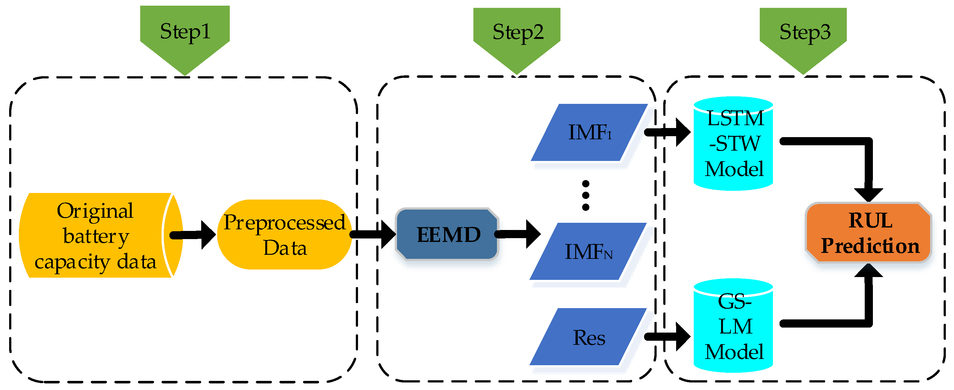
2. LSTM-STW and GS-LM (LSTM-STW-GS-LM) Fusion Prediction Method
- (1)
- The original battery capacity is preprocessed.
- (2)
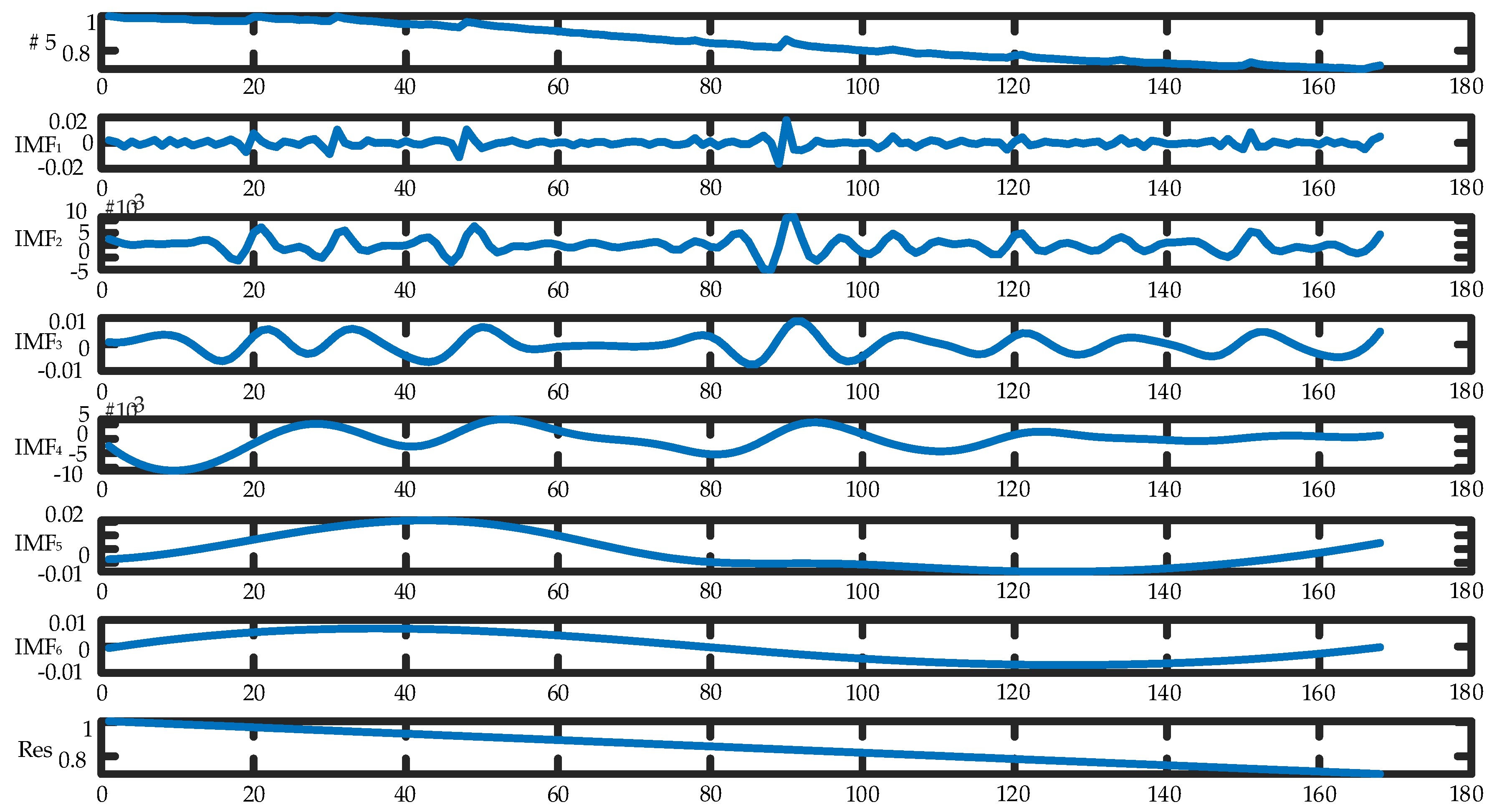
- The preprocessed data is decomposed into low-frequency and high-frequency data by EEMD.
- (3)
- The low-frequency prediction model is constructed by GS-LM, and the high-frequency prediction model is constructed by LSTM-STW. All the prediction results are integrated effectively to obtain the final combined prediction result.
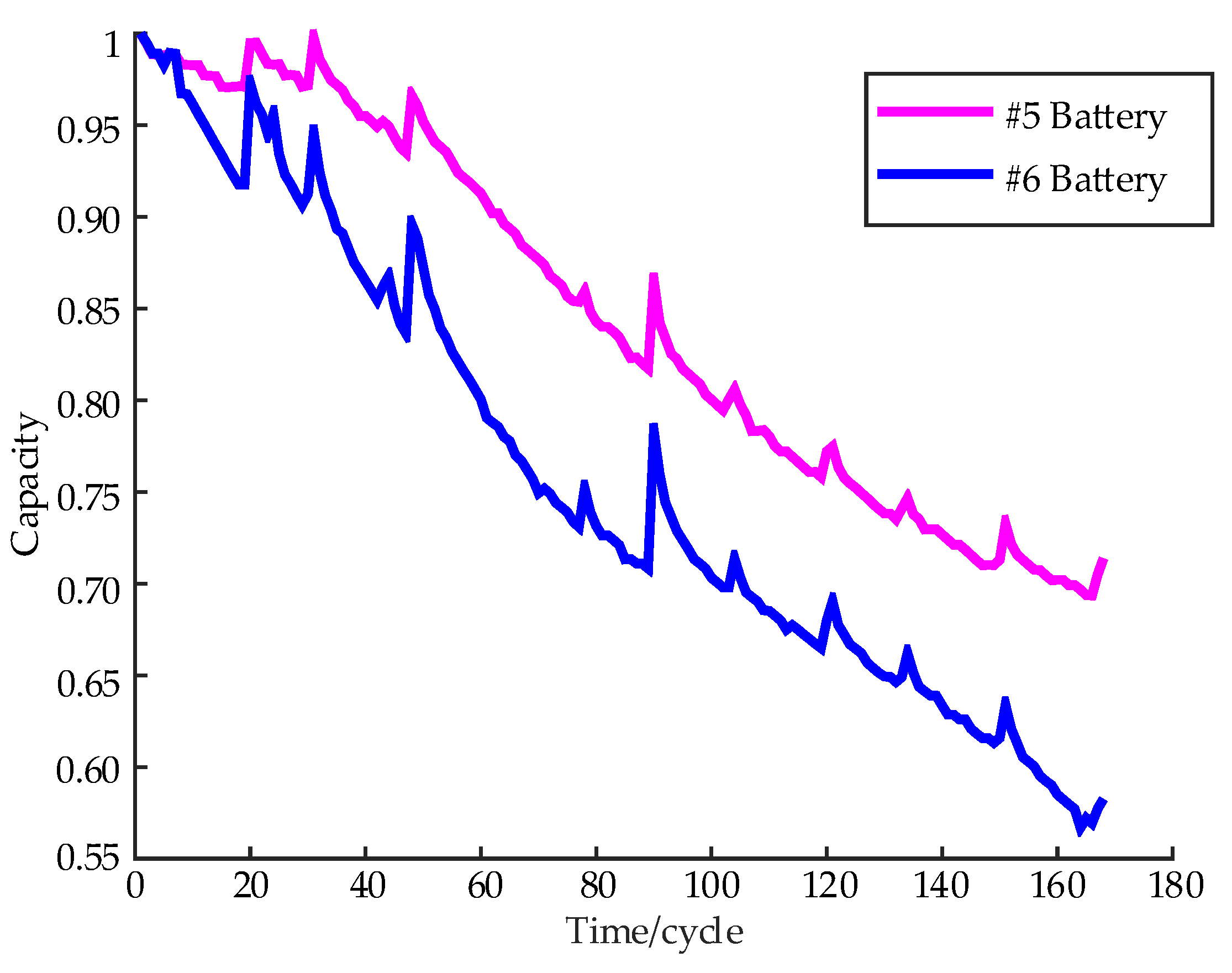
2.1. Experimental Data
2.2. Ensemble Empirical Mode Decomposition (EEMD)
- (1)
- the numbers of zero points and extreme points are equal or different by one for the entire data set;
- (2)
- the average value of the upper and lower envelopes at any location must be zero [23].
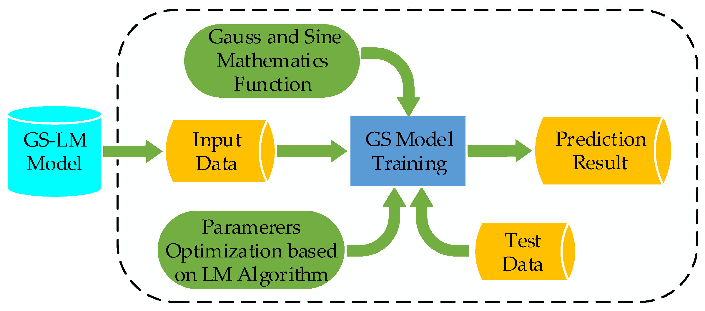
2.3. GS-LM Model
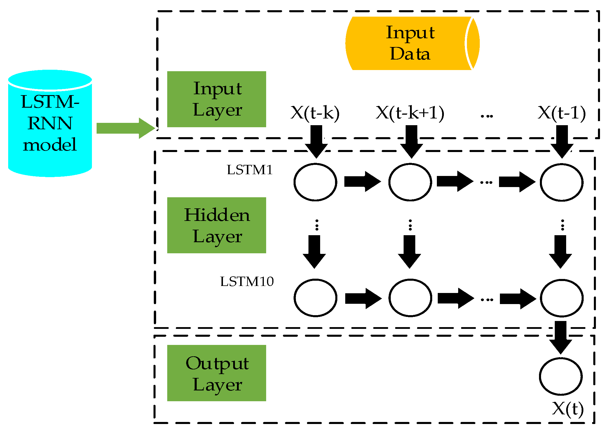
2.4. LSTM-STW Model
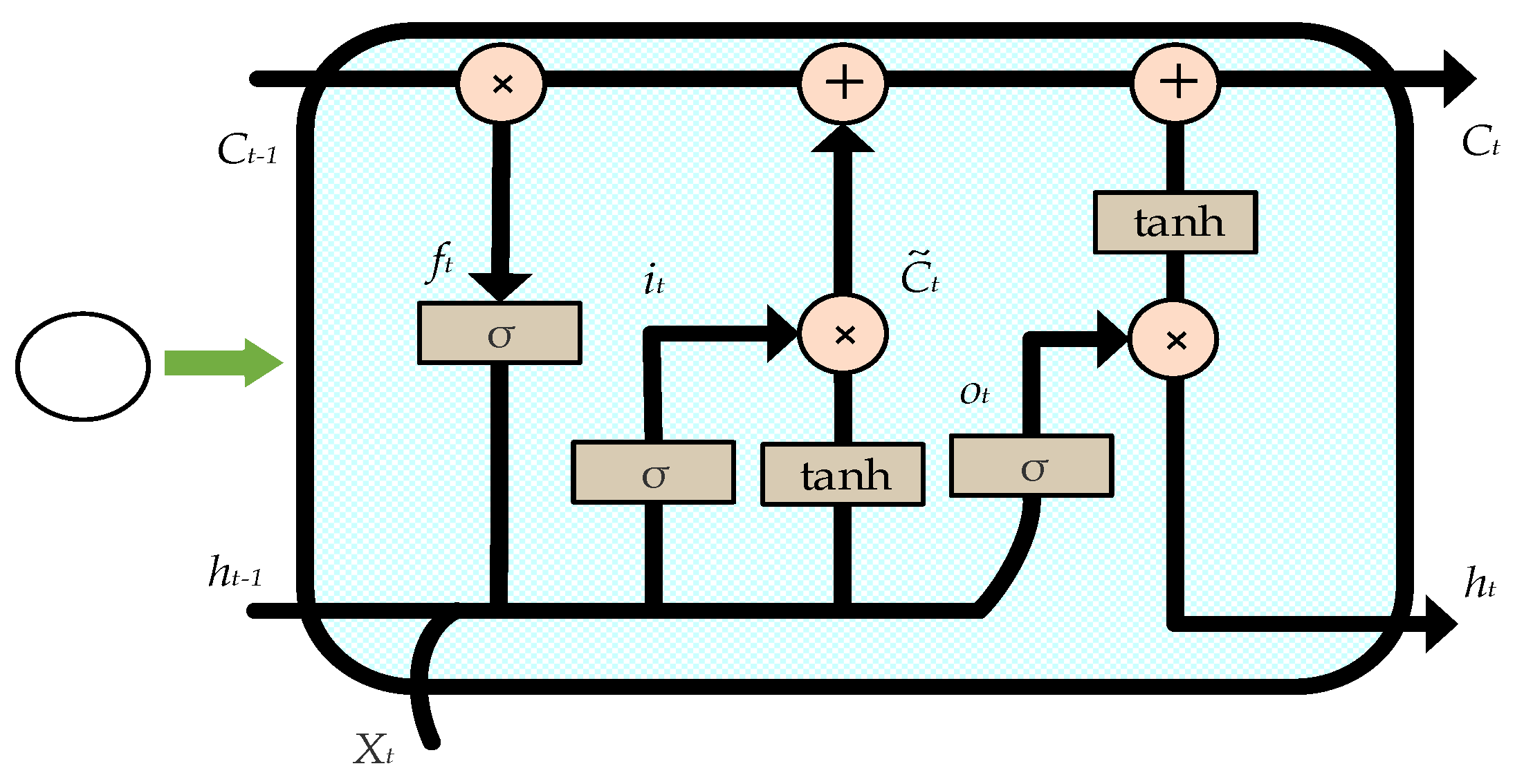
2.4.1. LSTM-RNN
- The forget gate: the first step and determines the information we will discard from the cell state.
- The input gate: it determines how much new information is added to the cell state.We can obtain short-term storage information of cells:
- Output gate determines the current output information:where Wf, Wi, WC, Wo is the parameter matrix, [ht−1, xt] is a matrix connected by two vectors ht−1, xt, bf, bi, bC, bo is the offset corresponding to each gate. σ and tanh are incentive functions as follows:
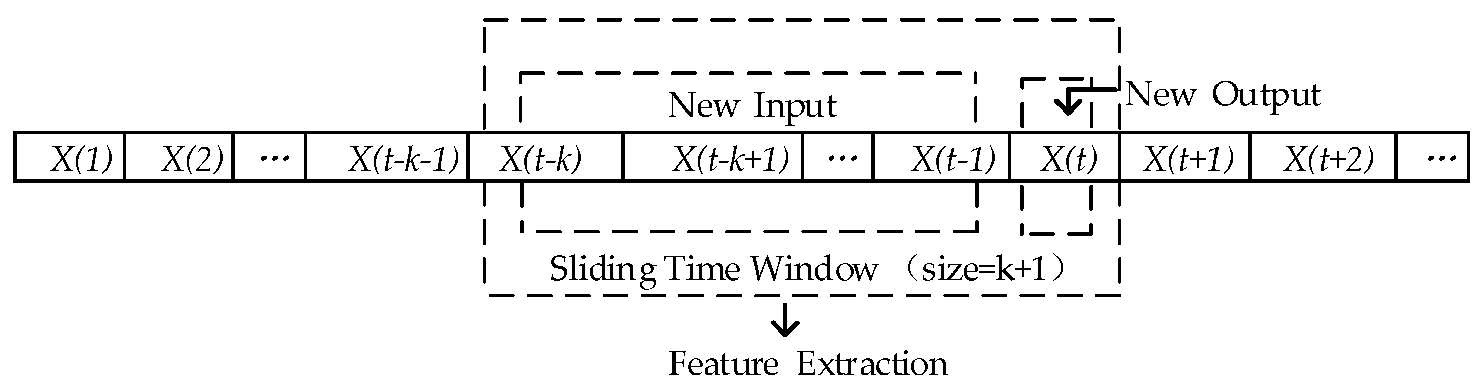
2.4.2. Sliding Time Window (STW)
3. Results and Discussion
3.1. Evaluation Criteria
- (1)
- the mean absolute percentage error (MAPE)
- (2)
- the mean absolute error (MAE)
- (3)
- the root mean square error (RMSE)
- (4)
- Errorwhere and stand for the battery charge capacity raw data and battery charge capacity prediction data, and s is the number of prediction data sets. EOL is the prediction starting point value. is the number of times used to predict the end of battery life.
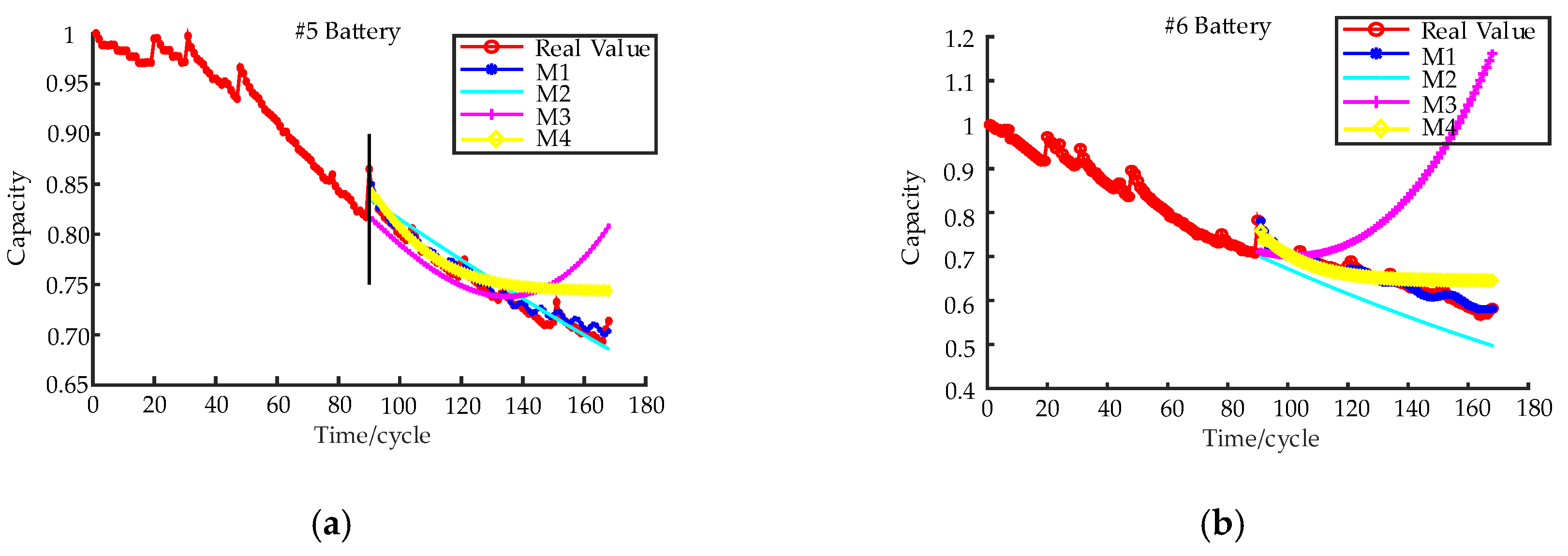
3.2. Experimental Results
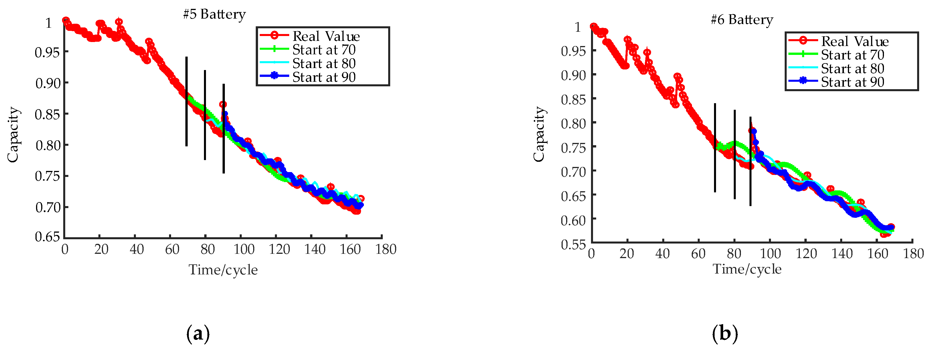
3.3. Different Prediction Starting Points
4. Conclusions
Author Contributions
Funding
Conflicts of Interest
Appendix A
- 1.
- According to the upper and lower extreme points of the synthesized signal S(n), draw the upper and lower envelopes Smax(n) and Smin(n), respectively, by cubic spline interpolation.
- 2.
- Find the average of the upper and lower envelopes and draw the mean envelope.
- 3.
- Subtract the mean envelope of the original signal to obtain the intermediate signal.
- 4.
- Determine whether the intermediate signal M(n) is IMF (using the above two conditions). If not, redo the analysis based on this signal 1–4.
- 5.
- After obtaining the first IMF1 using the above method, subtract the IMF1 from the original signal S(n) as the new original signal, and then analyze 1–4 to obtain IMF2, and so on until obtaining IMFN, S(n) subtracting IMFN is a monotonic function ResN(n), which is a complete EMD decomposition.
References
- Liu, D.T.; Zhou, J.B.; Guo, L.M.; Peng, Y. Survey on lithium-ion battery health assessment and cycle life estimation. Chin. J. Sci. Instrum. 2015, 36, 1–16. [Google Scholar]
- Lukic, S.M.; Cao, J.; Bansal, R.C.; Rodriguez, F.; Emadi, A. Energy storage systems for automotive applications. IEEE Trans. Ind. Electron. 2008, 55, 2258–2267. [Google Scholar] [CrossRef]
- Wu, Y.; Li, W.; Wang, Y.R.; Zhang, K. Remaining useful life prediction of lithium-ion batteries using neural network and bat-based particle filter. IEEE Access 2019, 7, 54843–54854. [Google Scholar] [CrossRef]
- Chen, J.J. Recent progress in advanced materials for lithium ion batteries. Materials 2013, 6, 156–183. [Google Scholar] [CrossRef] [PubMed]
- Chen, J.J.; Thangadurai, V. Frontiers of energy storage and conversion. Inorganics 2014, 2, 537–539. [Google Scholar] [CrossRef]
- Whittingham, M.S. History, evolution, and future status of energy storage. IEEE Proc. 2012, 100, 1518–1534. [Google Scholar] [CrossRef]
- Dubarry, M.; Svoboda, V.; Hwu, R.; Liaw, B.Y. Capacity and power fading mechanismidentification from a commercial cell evaluation. J. Power Sources 2007, 165, 566–572. [Google Scholar] [CrossRef]
- Zhang, Y.Z.; Xiong, R.; He, H.W.; Shen, W.X. Lithium- ion battery pack state of charge and state of energy estimation algorithms using a hardware-in-the-loop validation. IEEE Trans. Power Electron. 2017, 32, 4421–4431. [Google Scholar] [CrossRef]
- Saha, B.; Goebel, K.; Poll, S.; Christophersen, J. Prognostics methods for battery health monitoring using a bayesian framework. IEEE Trans. Instrum. Meas. 2009, 58, 291–296. [Google Scholar] [CrossRef]
- Xu, X.D.; Yu, C.Q.; Tang, S.J.; Sun, X.Y.; Si, X.S.; Wu, L.F. Remaining useful life prediction of lithium-ion batteries based on wiener processes with considering the relaxation effect. Energies 2019, 12, 1685. [Google Scholar] [CrossRef] [Green Version]
- Thomas, E.V.; Bloom, I.; Christophersen, J.P.; Battaglia, V.S. Rate-based degradation modeling of lithium-ion cells. J. Power Sources 2012, 206, 378–382. [Google Scholar] [CrossRef]
- Song, Y.C.; Liu, D.T.; Yang, C.; Peng, Y. Data-driven hybrid remaining useful life estimation approach for spacecraft lithium-ion battery. Microelectron. Reliab. 2017, 75, 142–153. [Google Scholar] [CrossRef]
- Zhang, H.; Miao, Q.; Zhang, X.; Liu, Z.W. An improved unscented particle filter approach for lithium-ion battery remaining useful life prediction. Microelectron. Reliab. 2018, 81, 288–298. [Google Scholar] [CrossRef]
- Zheng, X.J.; Fang, H.J. An integrated unscented kalman filter and relevance vector regression approach for lithium-ion battery remaining useful life and short-term capacity prediction. Reliab. Eng. Syst. Saf. 2015, 144, 74–82. [Google Scholar] [CrossRef]
- Long, B.; Xian, W.M.; Jiang, L.; Liu, Z. An improved autoregressive model by particle swarm optimization forprognostics of lithium-ion batteries. Microelectron. Reliab. 2013, 53, 821–831. [Google Scholar] [CrossRef]
- Parthiban, T.; Ravi, R.; Kalaiselvi, N. Exploration of artificial neural network [ANN] to predict theelectrochemical characteristics of lithium-ion cells. Electrochim. Acta 2008, 53, 1877–1882. [Google Scholar] [CrossRef]
- Zhang, Y.Z.; Xiong, R.; He, H.W.; Pecht, M.G. Long short-term memory recurrent neural network for remaining useful life prediction of lithium-ion batteries. IEEE Trans. Veh. Technol. 2018, 67, 5695–5705. [Google Scholar] [CrossRef]
- Pang, X.Q.; Huang, R.; Wen, J.; Shi, Y.H.; Jia, J.F.; Zeng, J.C. A lithium-ion battery rul prediction method considering the capacity regeneration phenomenon. Energies 2019, 12, 2247. [Google Scholar] [CrossRef] [Green Version]
- Li, X.Y.; Zhang, L.; Wang, Z.P.; Dong, P. Remaining useful life prediction for lithium-ion batteries based on a hybrid model combining the long short-term memory and Elman neural networks. J. Energy Storage 2019, 21, 510–518. [Google Scholar] [CrossRef]
- Wang, P.; Dan, X.; Yang, Y. A multi-scale fusion prediction method for lithium-ion battery capacity based on ensemble empirical mode decomposition and nonlinear autoregressive neural networks. Int. J. Distrib. Sens. Netw. 2019, 15, 1550147719839637. [Google Scholar] [CrossRef]
- Saha, B.; Goebel, K. Battery Data Set. Available online: https://ti.arc.nasa.gov/tech/dash/groups/pcoe/prognostic-data-repository/ (accessed on 20 September 2019).
- Wu, Z.H.; Huang, N.E. Ensemble empirical mode decomposition: A noise-assisted data analysis method. Adv. Adapt. Data Anal. 2011, 1, 1–49. [Google Scholar] [CrossRef]
- Zhang, C.Z.; Pang, H.P. A novel hybrid model based on EMD-BPNN for forecasting US and UK stock indices. In Proceedings of the 2015 IEEE International Conference on Progress in Informatics and Computing (PIC), Nanjing, China, 18–20 December 2015. [Google Scholar]


| Model | Description |
|---|---|
| M1 | the proposed method |
| M2 | double exponential model |
| M3 | cubic polynomial model |
| M4 | LSTM without using EEMD |
| Battery | Model | MAPE | MAE | RMSE | Runtime (Seconds) |
|---|---|---|---|---|---|
| #5 | M1 | 0.0072 | 0.0054 | 0.0066 | 37.6129 |
| M2 | 0.0136 | 0.0103 | 0.0119 | 2.2735 | |
| M3 | 0.0378 | 0.0274 | 0.0390 | 2.7154 | |
| M4 | 0.0244 | 0.0176 | 0.0232 | 5.8232 | |
| #6 | M1 | 0.0100 | 0.0065 | 0.0082 | 40.3431 |
| M2 | 0.0930 | 0.0596 | 0.0617 | 2.5987 | |
| M3 | 0.2920 | 0.1778 | 0.2490 | 2.9217 | |
| M4 | 0.0345 | 0.0210 | 0.0304 | 4.3176 |
| Battery | Prediction Starting Point | Error (Times) |
|---|---|---|
| #5 | 70 | 8 |
| 80 | 7 | |
| 90 | 2 | |
| #6 | 70 | 10 |
| 80 | 5 | |
| 90 | 1 |
© 2020 by the authors. Licensee MDPI, Basel, Switzerland. This article is an open access article distributed under the terms and conditions of the Creative Commons Attribution (CC BY) license (http://creativecommons.org/licenses/by/4.0/).
Share and Cite
Mao, L.; Xu, J.; Chen, J.; Zhao, J.; Wu, Y.; Yao, F. A LSTM-STW and GS-LM Fusion Method for Lithium-Ion Battery RUL Prediction Based on EEMD. Energies 2020, 13, 2380. https://doi.org/10.3390/en13092380
Mao L, Xu J, Chen J, Zhao J, Wu Y, Yao F. A LSTM-STW and GS-LM Fusion Method for Lithium-Ion Battery RUL Prediction Based on EEMD. Energies. 2020; 13(9):2380. https://doi.org/10.3390/en13092380
Chicago/Turabian StyleMao, Ling, Jie Xu, Jiajun Chen, Jinbin Zhao, Yuebao Wu, and Fengjun Yao. 2020. "A LSTM-STW and GS-LM Fusion Method for Lithium-Ion Battery RUL Prediction Based on EEMD" Energies 13, no. 9: 2380. https://doi.org/10.3390/en13092380