Integrated Transmission-and-Distribution System Modeling of Power Systems: State-of-the-Art and Future Research Directions

Abstract

Integrated transmission-and-distribution (T&D) modeling is a new and developing method for simulating power systems. Interest in integrated T&D modeling is driven by the changes taking place in power systems worldwide that are resulting in more decentralized power systems with increasingly high levels of distributed energy resources. Additionally, the increasing role of the hitherto passive energy consumer in the management and operation of power systems requires more capable and detailed integrated T&D modeling to understand the interactions between T&D systems. Although integrated T&D modeling has not yet found widespread commercial application, its potential for changing the decades-old power system modeling approaches has led to several research efforts in the last few years that tried to (i) develop algorithms and software for steady-state and dynamic modeling of power systems and (ii) demonstrate the advantages of this modeling approach compared with traditional, separated T&D system modeling. In this paper, we provide a review of integrated T&D modeling research efforts and the methods employed for steady-state and dynamic modeling of power systems. We also discuss our current research in integrated T&D modeling and the potential directions for future research. This paper should be useful for power systems researchers and industry members because it will provide them with a critical summary of current research efforts and the potential topics where research efforts are needed to further advance and demonstrate the utility of integrated T&D modeling.

1. Introduction

Computer-based modeling is critical to ensuring safe, reliable, and economic planning and operations of power systems. As the largest machine ever made, with highly complex, multitimescale (microseconds to several years) interactions, power system performance is not easily evaluated in realistic laboratory experiments. During the last 5–6 decades, several advancements have been made in simulating the engineering and economic performance of power systems via digital computers with high efficiency and reliability. The simulation approaches that were developed decades ago are still the workhorses of the power systems industry today, and these approaches have only changed a little. One reason for the incredible success of these algorithms is the small amount of change that has occurred to the power system itself during this time. The bulk of power generation still takes place at the level of the transmission system and, until recently, distribution feeders were also largely passive with little power generation. As a result, power systems analysis algorithms could artificially separate the two systems and solve transmission systems in detail with an extremely simple representation of the distribution networks and vice-versa.

In recent years, distributed generation (DG) has witnessed an exponential growth, particularly distributed photovoltaics (PV). This growth is expected to continue, and more DG types—including smart loads and electric vehicles—are expected to further fuel it. As the “center of gravity” of power generation shifts, and as DG penetration increases to an extent that distribution feeders inject power into the transmission system [1], there is increasing interest in improving the modeling of increased interactions between transmission and distribution systems. Research into new power system modeling techniques that can simulate transmission and distribution system interactions more effectively than the traditional approaches has been undertaken. Multiple approaches for modeling transmission and distribution systems together have been proposed, and several algorithms have been developed to perform steady-state and dynamic studies using integrated transmission and distribution (integrated T&D) system models. From this research, two key questions arise: What is the state of the art of research in integrated T&D modeling? Where should future research efforts be directed? Motivated by finding the answers to these questions, we performed a critical review of the current research in using integrated T&D systems for performing power systems analysis. We do not know of any other similar effort that has been undertaken so far, and we believe that this review will help researchers to obtain a better overview of the state of the art in integrated T&D modeling and help direct their research efforts to fill in gaps.

Any power systems analysis algorithm uses electrical engineering principles to properly simulate the phenomena of interest, and it uses computer science and mathematics principles for stability and convergence. The properties of the hardware on which the analysis is implemented—e.g., whether it can exploit multicore processing—are the software development aspects that are also critical for the success of a power systems analysis algorithm. In this review, we focus primarily on the algorithms that have been developed for integrated T&D modeling and not on software development. Moreover, there is increasing interest in expanding integrated T&D modeling to include simulations of other infrastructure components that have so far been ignored in power systems analysis; e.g., communications systems. Such multi-infrastructure simulations are also not considered in this paper because getting integrated T&D modeling right is the first critical step to ensuring the fidelity of multi-infrastructure simulations. Finally, regulatory changes that might be necessary to ensure the development and maintenance of integrated T&D models by electric utilities is also beyond the scope of this review. Figure 1 summarizes the integrated T&D topics that are discussed in this paper, and a short summary of the content discussed in this paper is provided next.

We review both steady-state and dynamic modeling using integrated T&D models in Section 2 and Section 3, respectively. An introduction to steady-state power systems analysis using integrated T&D models is provided first in Section 2.1, which is followed by a deep-dive into the research performed using unified integrated T&D models in Section 2.2 and using the co-simulation approach in Section 2.3. The discussion in Section 2.2 is centered around the three structures used for steady-state modeling under the unified integrated T&D modeling construct (TD-A to TD-C), whereas the discussion in Section 2.3 focuses on the various co-simulation approaches found in the literature and the key distinction between loosely and tightly coupled co-simulation approaches. Gaps in existing research on steady-state analysis using integrated T&D models and areas of future research are discussed in Section 2.4.

In Section 3, literature focused on studying electromechanical transients using integrated T&D models is reviewed because this has been the major focus of research performed so far on studying power systems dynamics using integrated T&D models. Two key conceptual challenges—at the time of initialization and during dynamic simulation iterations, encountered when studying electromechanical transients using integrated T&D models are discussed first in Section 3.1. This is followed by a discussion in Section 3.2 on the four structures (TD-1 to TD-4) found in literature for simulating dynamics using integrated T&D models. The literature review presented in Section 3.3 discusses the initialization approaches used with the TD-1 to TD-4 structures and how the initialization challenge is addressed or avoided in these approaches. Section 3.4 follows the same format as Section 3.3 but focuses on the dynamic simulation approaches used with TD-1 to TD-4 structures, i.e., how the power system is modeled to obtain the system state at the next time step. In Section 3.5, additional research efforts focused on the dynamic modeling of power systems using integrated T&D models are discussed. The key takeaways from Section 3.1–Section 3.5 and directions for future research in power system dynamics modeling using integrated T&D models are discussed in Section 3.6.

Section 4 concludes the paper with key takeaways from the paper and suggestions for future research.

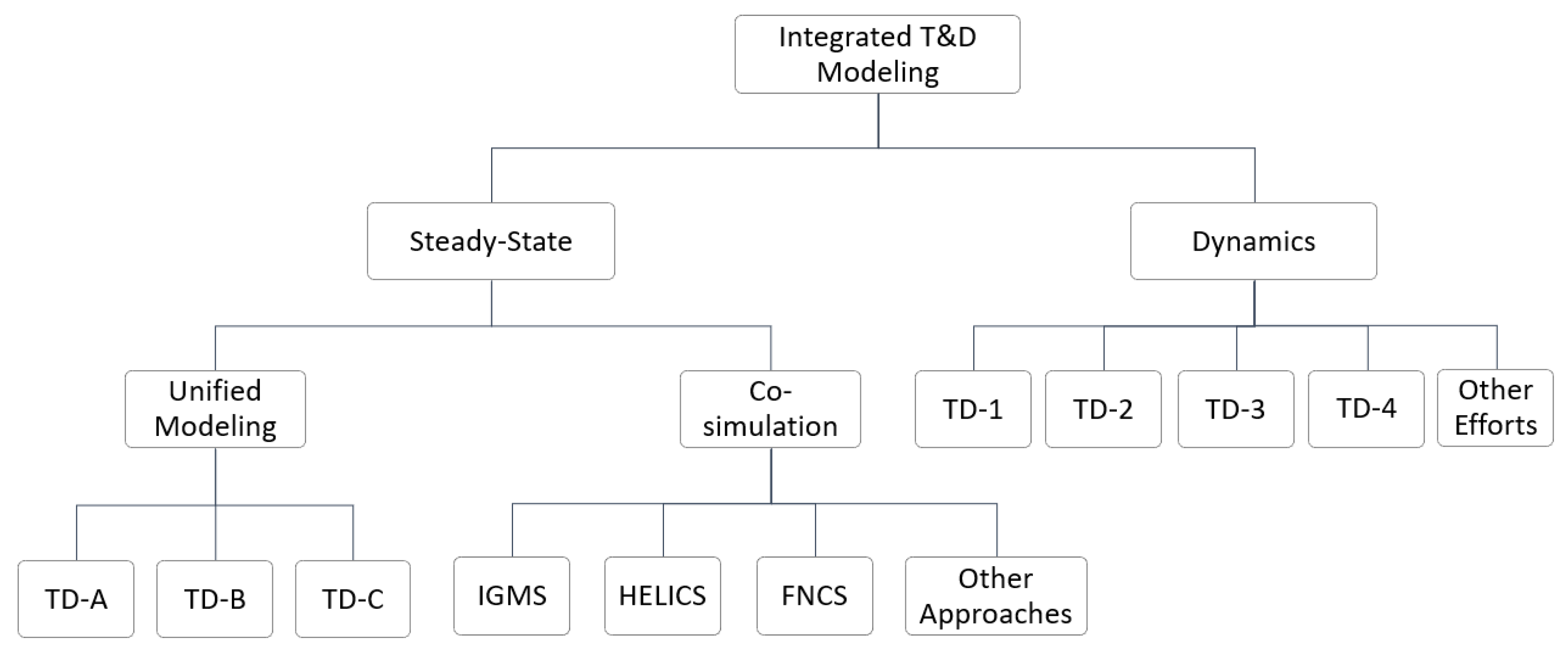
2. Steady-State Modeling of Power Systems Using Integrated T&D Models

2.1. Introduction

Traditionally, steady-state analysis of power systems has been performed separately for transmission and distribution systems. Legacy transmission system algorithms model distribution systems as balanced, lumped loads on transmission buses. Likewise, in distribution systems, the transmission system is typically modeled as a slack bus with constant balanced voltage. In the past, such modeling was justified under the assumptions that the transmission system is balanced, almost all generation is connected to the transmission network, and the power flow is unidirectional from the transmission system to the distribution system. Today, however, power systems are experiencing increasing penetration of distributed generation, a trend that is likely to continue into the foreseeable future, and which has attracted researchers’ attention to explore the integrated modeling of transmission and distribution systems. Some observations that further indicate the need to perform integrated T&D modeling include:

• Phase unbalance in transmission systems has been demonstrated for power systems with distributed energy resources (DERs) [2]. DERs can exacerbate phase unbalance in the distribution circuits to which they are connected. This unbalance gets reflected into the transmission system; hence, a balanced, three-phase operation cannot be assumed for the modern bulk power system.
• Bidirectional power flows exist between transmission and distribution systems [1,2].
• Steady-state voltage stability of transmission systems is a function of maximum load carrying ability of system buses [3], which in turn depends on the available generation resources, network topology, load patterns, and volt ampere reactive or Var support [4]. DERs connected to the distribution system impact these parameters, which leads to variability in voltage stability [5].

Consequently, there has been increasing consensus among the scientific and electric power communities on the need for integrated T&D modeling with high fidelity. To this end, several attempts have been made in recent years. These efforts for steady-state analysis can be classified into two categories: (i) those that focus on developing novel power flow techniques for solving a unified model of transmission and distribution systems and (ii) those that attempt to leverage existing, established legacy tools to solve separately modeled transmission and distribution systems through co-simulation. The next two sections discuss the algorithms and their applications to the two categories of integrated T&D modeling for steady-state analysis.

2.2. Unified T&D Model-Based Steady-State Modeling of Power Systems

Three different integrated T&D modeling structures (TD-A, TD-B, and TD-C) have been used by researchers for steady-state analysis. These are illustrated in Figure 2, and

Table 1. References that used the three integrated transmission-and-distribution (T&D) modeling structures for steady-state analysis.

T&D Modeling Structure	References Where Used
TD-A	[6,7,8,9,10,11]
TD-B	[12,13,14]
TD-C	[15,16]

summarizes the references where each structure has been adopted.

2.2.1. TD-A Approach

Most integrated T&D modeling efforts aim to create a novel power flow that can solve both transmission and distribution systems effectively. One such approach is to use Integrated Systems Models (ISMs) to model and simulate integrated T&D networks. The objective of the ISMs is to develop a common model of any system that can be modeled using “through” (e.g., current, fluid flow) and “across” variables (e.g., voltage, fluid pressure), where the common model manages and offers topology knowledge to algorithms, and where the common model has all measurements (e.g., from Energy Management Systems (EMS), Supervisory Control and Data Acquisition (SCADA), Advanced Metering Infrastructure (AMI)) attached and shared by all algorithms (more details about ISMs are provided in Appendix A). To perform steady-state analysis of transmission, distribution, or integrated transmission and distribution system models using the ISM approach, a matrix-free power flow for multiphase, unbalanced transmission and distribution networks was proposed in ref. [6]. This is based on a Graph Trace Analysis (GTA) approach. The framework was implemented using topology iterators and it enabled the separation of system equations from component equations. Further, the same topology iterators and algorithms were employed for transmission, radial distribution, lightly meshed distribution, and heavily meshed distribution systems. The solution speeds were not affected by changes in network topology as caused by the switching operations. It also provided the ability to distribute calculations across processors, and reported significantly faster computation times compared to matrix-based approaches (2.5–20 ×), depending on system characteristics [2,6].

Using the GTA-based approach, a steady-state voltage stability problem for integrated T&D systems was studied in ref. [7]. It demonstrated the use of a static, voltage stability margin index to identify weak links in the system, and it discussed methods to reinforce such links, leading to improved steady-state voltage stability. In ref. [8], using the same GTA-based solver, a dynamic control scheme was proposed to improve the steady-state load-carrying capability of buses by using distributed series reactors. The impact of PV variability on the steady-state voltage stability of integrated T&D systems was discussed in ref. [9]. Using GTA power flow, steady-state voltage stability heat maps were constructed, and the impact of PV generation loss and synchronous generator loss was quantified. In ref. [10], the authors used GTA to combine Gauss–Seidel and a continuation method into one algorithm to create a novel matrix-free power flow algorithm, GS-GTA. The algorithm was shown to be more robust than many Newton–Raphson (NR)-based algorithms. Moreover, the computational complexity of GS-GTA grows linearly with the size of the model. GTA, however, is still a relatively new concept for the power flow problem and it is an active research area.

The use of synthetic distribution system models for integrated T&D modeling was discussed in ref. [11]. The approach employed a top-down modeling approach and generated T&D models by combining transmission with synthetic distribution models. It used NR to solve integrated systems and demonstrated the usefulness of synthetic models for integrated T&D analysis; however, it was not clear how the poor convergence characteristics of the NR solver were handled for radial feeders. Additionally, the paper did not discuss the scalability and topology variation of the models.

2.2.2. TD-B Approach

A global power flow (GPF) method for integrated T&D systems based on the “master-slave” splitting concept was proposed in ref. [12], where structure TD-B was utilized. It solved the transmission power flow and the distribution power flow problems iteratively until the mismatches at the boundaries were within the tolerance. To improve convergence for distribution systems with loops, this paper also proposed an equivalent method. The proposed method is applicable for a three-phase model of both transmission and distribution systems. Further, the proposed method is compatible with existing power flow software. The accuracy and convergence of the proposed method were validated only using IEEE standard systems, with, at most, 118 transmission level buses and a few distribution feeders. The scalability of the proposed method was not demonstrated in this paper. In ref. [13], the authors expanded the work in ref. [12] for contingency analysis and proposed a GPF-based transmission contingency analysis method. It considered the “active” power flow of the distribution systems during the contingencies and evaluated the operational limits of both transmission and distribution systems. To reduce the communication burden between transmission and distribution control centers and to improve computational efficiency, the authors introduced three approaches for speeding-up the simulations—contingency selection beforehand, direct-current power flow approximation, and the equivalency of the distribution system, assuming no communication between transmission and distribution systems. Switching back to the traditional contingency analysis method was suggested in the case of divergence. As in ref. [12], this paper did not show the scalability of the proposed contingency analysis method for large-scale power systems.

A diakoptics-based mixed-modeling framework was proposed in ref. [14] for analysis using integrated T&D models. This can represent the unbalanced conditions at the boundaries by modeling the transmission system as one subsystem using decoupled positive, negative, and zero sequence models, while modeling the distribution systems connected to it in three-phase. It solved power flow iteratively between transmission and distribution systems, based on the master-slave concept as in ref. [12], but it also developed a three-sequence power flow algorithm for solving the transmission system. If decoupled sequence matrices are used, this approach will not accurately handle transmission systems with untransposed lines.

2.2.3. TD-C Approach

A combined T&D steady-state simulation framework is proposed in ref. [15], which models the transmission system as a positive sequence network and the distribution system as a three-phase network. This employs the equivalent circuit models for transmission and distribution systems, and subsequently uses coupling circuits to combine the two. The coupling circuits model a P-Q or load bus using a complex current source that is split into real and imaginary current sources to enable the application of the NR solver. The current of this complex source is a function of the load bus voltage. The proposed framework solves the smaller combined T&D networks (<1 × 10⁶ nodes) on a single machine with a direct NR solver, whereas larger combined T&D networks (>1 × 10⁶ nodes) are solved in parallel using a parallel Gauss–Seidel–Newton solver on multiple cores. This work, however, assumes a balanced transmission system, and thus it solves only the positive sequence transmission network model. Additionally, the authors claimed the convergence of the NR solver for T&D models. Because it is well-known that the NR solver exhibits poor convergence characteristics for radial distribution circuits [17,18], it is not clear how the framework accounted for these characteristics of the NR solver. Moreover, the work considered only static models with fixed topology. Handling topology change is desirable because it can result from network reconfiguration after fault/contingency or from switching operations on a feeder. Building a single matrix for the integrated T&D system to apply the NR methods becomes computationally expensive, and multiple cores are needed to solve larger systems. Similarly, in ref. [16], the authors proposed an equivalent circuit formulation approach with current and voltage variables that models both the positive sequence network of the transmission network and the three-phase network of the distribution network. Then, a novel algorithm combined the equivalent models to generate an equivalent T&D model that was solved. The algorithm was used to solve a 75k+ node eastern interconnection transmission test case, and an 8k+ node taxonomy distribution test case starting from arbitrary initial guesses. As in ref. [15], this work considered static models without any changes in topology caused by system operations. Additionally, it also modeled the transmission system as a positive sequence network.

2.3. Co-Simulation Approach for T&D Model-Based Steady State Modeling of Power Systems

In recent years, several co-simulation-based approaches have been reported for integrated T&D modeling. These methodologies model and simulate T&D models using their respective specialized domain-specific tools while exchanging the time-synchronized boundary conditions. Because this approach uses mature and established legacy power flow tools, it offers domain expertise as compared to a novel generic power flow for solving an entire T&D model. On the other hand, using established legacy tools results in their limitations being inherited in co-simulations. For example, by using transmission network modeling software that assume the network is balanced, any unbalance at the transmission and distribution interface is not propagated into the transmission system. Moreover, untransposed transmission lines cannot be modeled. The discussion that follows presents various co-simulation-based integrated T&D modeling efforts that we found in literature.

2.3.1. Integrated Grid Modeling System

The Integrated Grid Modeling System (IGMS) reported in ref. [19] uses Python- and Message Passing Interface (MPI)-based cores to time-synchronize and co-simulate transmission systems modeled in MATPOWER [20] with distribution systems modeled in GridLAB-D [21]. IGMS simulations of integrated T&D systems (>1 million buses) demonstrated that increasing grid operator visibility and forecasting for distributed PV can reduce production costs and improve reliability.

A study on the impact of DG from solar photovoltaics (DGPV) was performed in ref. [22] using IGMS and a 5-bus transmission and 11-feeder distribution synthetic integrated T&D model. This study demonstrated the importance of DGPV forecasting for system operations at the transmission level, and the value of integrated T&D over distribution-only simulations on distribution voltage profiles and regulations, especially under high DGPV penetration levels.

In ref. [23], the impact of price-responsive load (PRL) on power systems was evaluated using IGMS and the same 5-bus transmission and 11-feeder distribution synthetic integrated T&D model. In the integrated T&D model, the price-responsive behavior of individual loads connected in the distribution feeders was modeled using the passive controller of GridLAB-D [24]. Because of the absence of the distribution network in the transmission-only model, the price-responsive behavior of the aggregate loads at the transmission buses was modeled using own-price elasticities. This study showed that an integrated T&D model can provide a better view of the behavior of PRLs and simulate their impact more accurately than a transmission-only model because it can only make assumptions regarding the aggregate price-responsive behavior of PRLs, instead of modeling them individually.

2.3.2. Hierarchical Engine for Large Scale Infrastructure Simulation

In ref. [25], the Hierarchical Engine for Large Scale Infrastructure Simulation (HELICS) [26] was used to co-simulate Transmission, Distribution, Communication, and Control simulators. HELICS is an open-source, co-simulation framework with interface application programming interfaces available for many domain-specific tools and programming languages. It is a scalable, high-performance, cross-platform tool with multiple simulation options, including discrete event, quasi-steady-state simulations (QSTS), and dynamic simulations.

2.3.3. Framework for Network Co-Simulation

In ref. [27], the authors proposed a transactive energy simulation platform using the Framework for Network Co-Simulation (FNCS) [28]. The platform co-simulates Energyplus^TM [29] for buildings with MATPOWER for transmission systems, GridLAB-D for distribution systems, and Python-based agents for grid edge devices. It defines several economic metrics for evaluating transactive energy mechanisms, and it proposes multiple improvements to the time-simulation environment that is deployed to evaluate transactive case studies. FNCS is a predecessor of HELICS, and it can be regarded as the lightweight version of HELICS. Contrary to HELICS, FNCS assumes a loose coupling among interacting tools. Loose and tight coupling in co-simulations are important concepts that are discussed next.

2.3.4. Loose and Tight Couplings in T&D Co-Simulation

Loosely coupled co-simulation frameworks assume that the changes in the power system are rather slow, and thus they exchange boundary variables in subsequent time steps until the system converges over multiple time steps. When studying T&D control coordination and similar behaviors with faster dynamics, however, tight coupling is desired where the system boundary variables are visualized for convergence at each time step. Thus, the time step for tightly coupled systems advances only once the boundary variables converge. This concept is often referred to as co-iteration at each time step. HELICS supports co-iteration or tight coupling among the interfaced tools. The T&D coupling topologies are depicted in Figure 3.

2.3.5. Other Co-Simulation Approaches

Some other co-simulation-based integrated T&D studies include [30] in which authors propose an iterative framework to tightly couple the transmission and distribution networks at each iteration of co-simulation. A three-phase transmission system model was developed and coupled with a distribution system for unbalanced system analysis. For time-synchronization and information exchange, a MATLAB based interfacing application was developed, and advantages of tightly coupled systems over loosely coupled systems were demonstrated. Model convergence was slow, however (7–11 s for a single iteration in tight coupling). Additionally, there was no mention of scalability for this framework and how the solution time evolved with system size. Moreover, models with changing topology were not discussed.

The authors suggested an improvement in ref. [31], where they proposed a serial implementation of the framework previously implemented in parallel [30]. The improved serial implementation reduced the required iterations by half. Moreover, the authors discussed and compared the transmission and distribution coupling protocols for co-simulation, i.e., decoupled (separately simulated transmission and distribution systems), loosely coupled (without co-iteration), and tightly coupled (co-iteration). The authors also reported that the accuracy of both decoupled and loosely coupled models deteriorates with increasing system unbalance, DER penetrations and variability, and the number of T&D coupling nodes. The authors suggested using tightly coupled protocols for co-simulating T&D models because they more closely approximate real-world systems. Similar findings were reported in ref. [32], where tightly coupled systems were benchmarked against loosely coupled systems. The authors discussed quasi-static co-simulation for steady-state power flow; hybrid co-simulation to evaluate frequency regulation issues, and dynamic co-simulation to model transients/faults.

A discussion of multi-point T&D coupling while considering distribution system loops was presented in ref. [33]. The work demonstrated that co-simulation was possible even when transmission nodes were coupled through a distribution network; however, it requires modifying the transmission system model to reflect the additional current paths. Instead of using the positive-sequence approximation, the transmission systems were modeled in distribution-coupled three sequences by placing equivalent branches in the transmission model and accounting for loop currents.

Table 2. Numerical comparison of algorithms used to model and solve the steady-state integrated T&D networks.

References	T&D Structure Used	Reference Software	Largest Network Tested	Synthetic */Utility Model	Time in Seconds to Solve One Power Flow (for the Largest Network)	Discussion on Numerical Stability/Convergence of Algorithm?
[6,7,8,9,10]	TD-A	Distributed Engineering Workstation (DEW)	Network model with 784,000 nodes and 8 voltage levels	Utility	21	Yes
[11]	TD-A	Custom Tool	System with 1076 buses	Synthetic	120	No discussion found
[12,13]	TD-B	Custom Tool	System with 118 transmission buses and 6 feeders with 44 nodes	Synthetic	Not mentioned. It only discusses iterations	Yes
[20,21]	TD-C	Custom Tool	Eastern Interconnection system with 75,000 nodes	Utility	0.4	Yes
[19,22,23]	Co-simulation	GridLAB-D and MATPOWER (IGMS)	1.3 million buses	Utility	46,388	Yes
[25]	Co-simulation	HELICS	Entire island of Oahu, HI with >1 million nodes	Utility	Not mentioned	Yes
[26]	Co-simulation	FNCS, Energyplus, MATPOWER	9 bus transmission model with multiple distribution feeders	Synthetic	Not mentioned	Yes
[30,31,32]	Co-simulation	MATLAB	IEEE 39 bus transmission and EPRI Ckt-24 distribution feeder	Synthetic	7–11	Yes

* Synthetic model means that it does not represent the network of an actual utility.

presents a numerical comparison of the approaches for steady-state integrated T&D modeling and simulation that were discussed earlier.

2.4. Gaps and Future Research Directions

• Quantifying the value of performing steady-state analysis using integrated T&D models. Improved modeling accuracy is an obvious advantage of using integrated T&D models. However, as the above review revealed, researchers have adopted different approaches, each with its own advantages and limitations, and we are unaware of a thorough evaluation of these approaches to quantify the relative costs and benefits of each. Moreover, there is an inherent cost involved in shifting to new tools (e.g., because of personnel training and the development of new databases). This cost must be justified to stakeholders who might want to adopt this new modeling and simulation paradigm. Defining metrics to quantify the costs and benefits of integrated T&D modeling can help stakeholders make informed choices about the algorithms and integrated T&D modeling approaches they wish to adopt.
• Developing tools and techniques to analyze data generated by time series simulation of large integrated T&D models. Real-world, integrated T&D models can comprise millions of nodes and generate hundreds of gigabytes of data. Moreover, new patterns or phenomena might be buried in the data that power system planners and operators have not encountered before in separate transmission and distribution modeling. Manual data processing to sift through such large datasets and identifying the new patterns that these data might contain can be very difficult, if not impossible. This has not been the focus of research so far, and research that aims to develop techniques and tools to process the vast quantities of data generated in integrated T&D modeling can help to further the adoption of this new paradigm for power systems modeling.
• Developing T&D simulators for hardware-in-the-loop simulations. Hardware-in-the-loop simulators emulate characteristics of the real system and thus facilitate equipment integration. T&D hardware-in-the-loop simulators could provide useful insights into the behavior of the integrated system when dealing with disturbances, renewable generation variability, and faults. Developing such simulators is not trivial; however, because of the immense scale and details associated with integrated T&D system models.
• Lack of validation standards and models for testing/benchmarking novel T&D power flow algorithms. For benchmarking a novel power flow algorithm, IEEE standard models can be used; however, these models are for only transmission or distribution. There is no standard model that can be used to benchmark the performance of a novel T&D power flow algorithm. Recently, a public, synthetic integrated T&D dataset was developed, which can be accessed here [34].
• Most integrated T&D simulations require extensive computing resources. Thus, improving the efficiency, speed, and convergence time of these algorithms—whether by improving the algorithms themselves or by parallel processing and distributed computations—remains a gap that needs to be addressed.

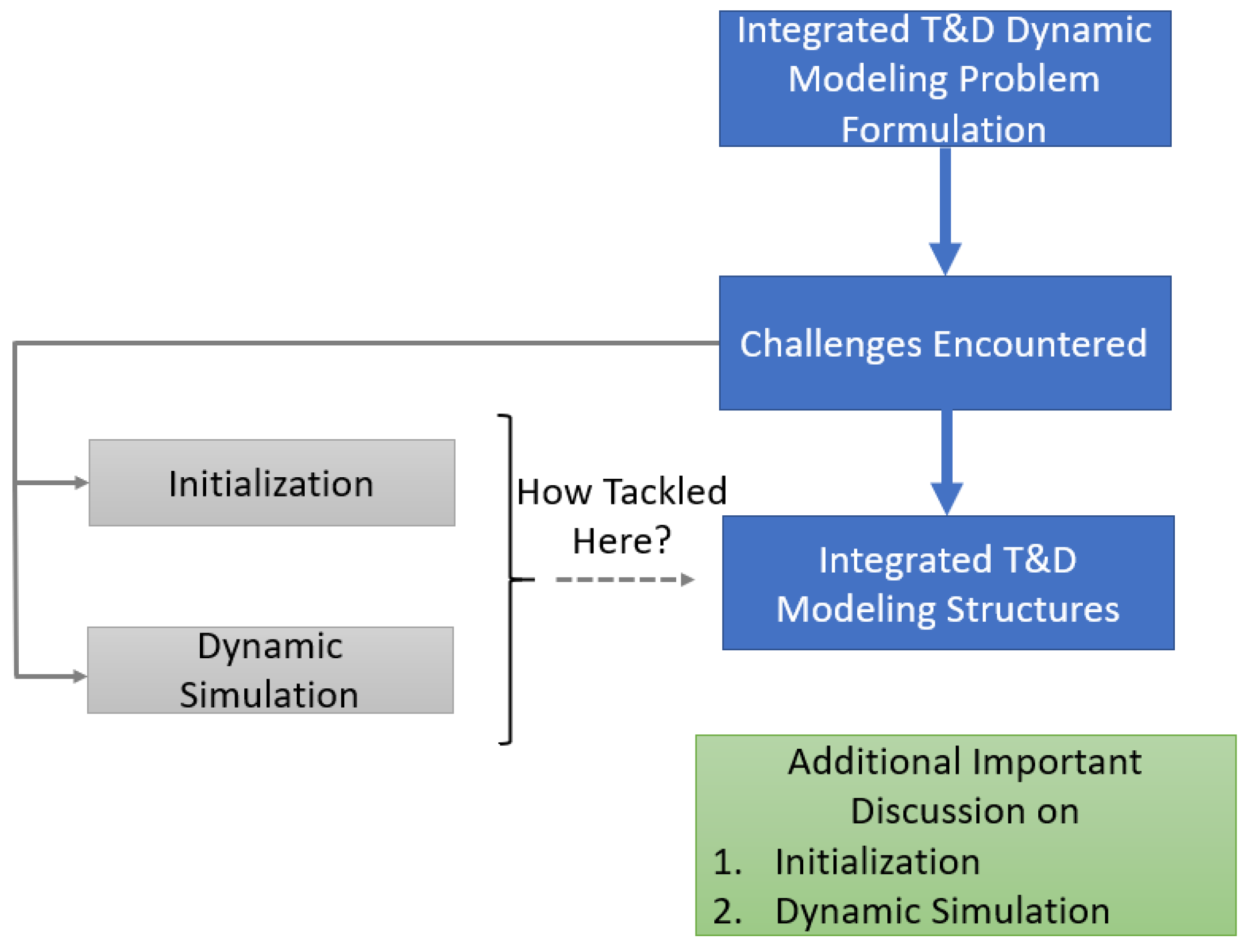
3. Dynamic Modeling Using Integrated T&D Models

This section reviews the work done on integrated T&D dynamic modeling for studying system stability under electromechanical transient timeframes, because these transients have been the predominant focus of research aimed at simulating power system dynamics using integrated T&D models.

The general power system model used in integrated T&D dynamic simulations is very similar to the Differential Algebraic Equations (DAE)-based model, used in traditional dynamic simulations [35]. In other words, network transients are neglected, and the network is assumed to transition from one steady-state to the other instantaneously. Slower dynamics associated with electrical machines, inverters (if neglecting inner control loops), and loads are modeled using differential equations. Equation (1) gives the general form of the DAE equations.

$$\begin{array}{c}\dot{x}=f\left(x,y,u\right)\\ 0=g\left(x,y,u\right)\end{array}$$

(1)

where $x$ is the set of dynamic state variables; $y$ represents the algebraic state variables; $u$ represents the external inputs, such as power references for governors; $f$ is the set of derivatives of the state variable set $x$; $g$ represents the set of algebraic equations.

DAE-based modeling for integrated T&D models, however, presents some unique challenges that are not encountered with the DAE models of balanced transmission systems. The review presented in the following sections is motivated by these challenges, which are discussed in Section 3.1. This is followed by a detailed discussion on the modeling structures used for dynamic modeling using integrated T&D models and how these challenges are mitigated or avoided. Figure 4 shows the organization of the review on dynamics modeling using integrated T&D models.

3.1. Key Challenges of Integrated T&D Dynamic Simulations

The first step in any dynamic simulation is the initialization of the dynamic state variables. The typical approach is to start the initialization from the solved power flow. The voltages and currents at the terminals of all the dynamic models that interface directly with the network are used to initialize all the dynamic states. Conceptually, in steady state, which is what the initial power flow represents, the derivatives of all state variables should be zero. In other words, solving (1) with $\dot{x}$ set to zero gives the initial states of all the dynamic models. Moreover, barring numerical instability or an unstable operating point, or a dynamic model initialized in the nonlinear region, all states should stay unchanged post initialization until a disturbance is applied. In large system models, perfect initialization is seldom achieved, but the states typically do not differ much from their initial values until a disturbance is applied. Therefore, for a balanced system, initialization, based on initial power flow, poses no problems. Now, let us see what happens when (1) is used in integrated T&D dynamic simulations where the assumption of system balance no longer holds.

To motivate this discussion, consider differential Equations (34)–(42) governing the two axis synchronous generator model given in ref. [36].

At the time of initialization, the $dq0$ axis voltages are obtained from the initial power flow after applying the Park’s transformation. When the system is balanced, the $dq0$ axis voltages and currents are simply obtained from Equations (2) and (3), with the zero-axis voltage being zero [35].

$$v_d+j{v}_q=V^{j\left(\theta -\delta +\frac{\pi }{2}\right)}$$

(2)

$$i_d+j{i}_q=I^{j\left(\alpha -\delta +\frac{\pi }{2}\right)}$$

(3)

where $V$ is the voltage phasor magnitude, $\theta$ is the voltage phasor angle, and $\delta$ is the initial rotor angle. Similarly, $I$ and $\alpha$ are the current phasor magnitude and angle, respectively. Because $\delta$ is unknown at the time of initialization, it is calculated by solving differential Equations (34)–(42) in ref. [36] with their derivatives set to zero. It is not difficult to show that the initialization results in constant or non-time-varying $\delta$, which means that $v_d$ and $v_q$ are also non-time-varying constants.

When the network is unbalanced, however, several changes happen:

• Although the average value of three-phase power is constant in steady-state, the instantaneous power oscillates at twice the fundamental frequency. In a balanced system, the instantaneous three-phase power is also constant.
• Because power oscillates at twice the fundamental frequency, so does the torque seen by the generators [37,38] and hence the rotor angle [38].
• Even if the oscillations in the load power and the resulting torsional oscillations in the generators are ignored and the rotor angle $\delta$ is assumed to be constant, application of the Park’s transformation at steady-state frequency shows that the $d$ and $q$ axis voltages and currents have oscillatory components superimposed on DC values. Equation (4), copied from [36], shows how the oscillatory components appear in the $d$ and $q$ axis voltages under network unbalance.

$$\left[\begin{array}{c}{v}_d\\ v_q\\ v_0\end{array}\right]=\sqrt{2}\left[\begin{array}{c}0\\ 0\\ \left|V_0\right|\cos ({\theta }_0+{\omega }_{s}t)\end{array}\right]+\sqrt{2}\left[\begin{array}{c}\left|V_{+}\right|\sin \left(\delta -{\theta }_{+}\right)\\ \left|V_{+}\right|\cos \left(\delta -{\theta }_{+}\right)\\ 0\end{array}\right]+\sqrt{2}\left[\begin{array}{c}\left|V_{-}\right|\sin \left(\delta +{\theta }_{-}+2{\omega }_{s}t\right)\\ \left|V_{-}\right|\cos \left(\delta +{\theta }_{-}+2{\omega }_{s}t\right)\\ 0\end{array}\right]$$

(4)

where, $V_{+}^{j{\theta }_{+}}, V_{-}^{j{\theta }_{-}}, and V_0^{j{\theta }_0}$ are the positive, negative and zero sequence components of the terminal voltage.

The last point shows that, even if constant rotor angle is assumed under network unbalance, time-varying voltages and currents will appear in differential Equations (34)–(42) of [36]. Reference [38] showed that twice the fundamental frequency oscillations appear in all rotor field variables. Under these conditions, setting the derivative to zero in differential Equations (34)–(42) of [36] to obtain the “fixed” points is incorrect. Mathematically, these equations behave as a non-autonomous system of ordinary differential equations (ODEs) because of their explicit dependence on time. Fixed points do not exist for such systems [39]; therefore, assuming that the derivatives are zero at steady state is incorrect, and different approaches for initializing T&D dynamic simulations of the form (1), or even distribution-only dynamic simulations of the type (1), are required.

The unbalanced network poses another challenge during T&D dynamic simulation when (1) is used to model the dynamic system. When the network is balanced, (2) and (3) can be used to obtain the terminal voltage and current phasors after each integration time step using the time domain $d$ and $q$ axis voltages and the rotor angle, $\delta$. When the network is unbalanced, three unique terminal voltage or current phasors must be calculated after each integration step. Only three time-domain values are, however, available, i.e., the $d$-, $q$-, and $0$-axis voltages or currents, which are not sufficient to obtain three unique voltage or current phasors. Researchers have developed different approaches to solve or circumvent this problem. These approaches and the trade-offs they have made between accuracy and simplicity are discussed in the next section.

3.2. T&D Dynamic Simulation Models Used in Literature

How researchers attempt to solve these challenges is intimately tied to the structure they adopt for integrated T&D dynamic modeling. Figure 5 shows the four structures found in the literature, and

Table 3. References that used the four T&D dynamic modeling structures.

T&D Modeling Structures	Pros	Cons	References Where Used
TD-1	Most accurate dynamic modeling	Re-use of existing dynamic simulation software is difficult	[36,40,41,42,43]
TD-2	Domain-specific existing dynamic simulation software can be used	Modeling of un-transposed transmission lines is difficult	[14,44]
TD-3	Existing balanced transmission system dynamic models can be used	Transmission system unbalance cannot be modeled, resulting in inconsistent interface between transmission and distribution systems	[45,46]
TD-4	Existing balanced transmission system dynamic models can be used	Only applicable where distribution systems can be assumed to be balanced	[47]

lists the references where each structure was used. The discussion that follows this section relies heavily on these modeling structures.

3.2.1. TD-1 Structure

In TD-1, the entire transmission and distribution network is modeled in three phase and in a single software, the Distributed Engineering Workstation (DEW) [48]; therefore, the transmission and distribution interface mimics the one that exists in the field. The TD-1 structure is identical to the TD-A structure previously discussed. The key advantage of modeling the transmission and distribution network in a dynamic system in the form of TD-1 is that unbalance in both transmission and distribution networks and the resultant impact on transmission and distribution dynamics can be simulated. Potential concerns that have been raised for such an approach are (i) the inability to use existing and widely used tools, (ii) the scalability, and (iii) the computational complexity and speed [14,46]. As shown in ref. [49], however, GTA [50], which forms the backbone of the TD-1 structure in refs. [36,40,41,42], can be parallelized to significantly improve the scalability and computational speed to solve both radial and networked multi-phase distribution systems. Moreover, the transmission system can be split into several sub-systems, each of which can be solved on a separate node of a multi-processor machine and the individual sub-systems results are then used to solve the entire system. The promise of such a diakoptics approach implemented on a cluster computing platform, when compared to sparsity based techniques, is highlighted in ref. [51]. In ref. [43], the transmission and distribution systems are also modeled as a unified system in MATLAB/Simulink [52].

3.2.2. TD-2 Structure

In TD-2, the transmission network is proposed to be simulated in three sequences without any coupling between the sequence networks, whereas the distribution network is modeled as an unbalanced three phase network. It is further proposed that the transmission and distribution networks interact using a multi-area Thevenin equivalent, or MATE, approach. In MATE, a network is split along desired boundaries and each such subsystem is solved separately. Then, each subsystem’s multipoint Thevenin equivalent—as seen at the link branches where the subsystem was split from the rest of the network—is assembled, and the reduced system is solved to obtain the link branch currents that are then used to update the solution of each individual subsystem. The MATE method was described in detail in refs. [51,53] for solving linear and nonlinear networks.

In the TD-2 approach presented in refs. [14,44], the MATE approach was used to split only distribution networks at each location where they would connect to a transmission network. Moreover, although the entire transmission network was solved in three sequences, the distribution networks were solved in three-phase and then converted to a three-sequence representation for the consistent solution of the MATE-based combined T&D network to obtain the link currents. The main advantage of the TD-2 interface is that T&D networks can be solved in different software and brought together through the MATE interface, which allows for existing specialized domain-specific software to be used to solve transmission and distribution networks. The main disadvantage of TD-2 is that the decoupled three-sequence transmission representation does not allow for untransposed transmission lines to be modeled, though the authors point to, but do not use, an approach that allows asymmetrical transmission lines to be modeled in three-sequence power flow [54].

3.2.3. TD-3 Structure

TD-3 [45,46] is a simple T&D interface where the transmission network is assumed to be balanced while the distribution network is modeled as an unbalanced three-phase network. The transmission network is presented to the distribution network as a stiff balanced voltage source at the distribution substation, whereas the total three-phase power at the distribution substation is presented to the transmission network as balanced three-phase power. The biggest advantage of this approach is that the transmission system dynamics can be solved using existing approaches; however, inaccuracies arising from neglecting the unbalance in the transmission network cannot be avoided. Moreover, distribution network DAEs face the same initialization and unbalanced voltage phasor calculation challenges as discussed in the previous section. If the distribution network is modeled as ODEs instead of DAEs in an electromagnetic transient (EMT) program, as in ref. [45], then the voltage phasor calculation challenge can be avoided, though the initialization challenge will still remain if the initial power flow-based initialization approach is followed; however, long simulation times for simulating a realistic distribution network in an EMT program [55] is the main drawback of this approach.

3.2.4. TD-4 Structure

TD-4 was presented in ref. [47]. This is the simplest approach to modeling power system dynamics using integrated T&D systems. Traditional methods for solving (1) that are used for the transmission system can also be used to solve integrated T&D systems modeled as TD-4. Simplicity and the use of existing software and simulation approaches are the key benefits of this modeling approach. The key limitation is the limited applicability to regions where distribution networks are balanced.

3.3. Initialization

Aside from TD-4, the initialization challenge will be encountered in TD-1 to TD-3 modeling structures if the dynamic models connected to transmission and/or distribution systems are initialized based on unbalanced power flow. Let us now consider how researchers have tried to address this problem.

3.3.1. TD-1 Initialization

As discussed, the TD-1 structure was adopted in refs. [36,40,41,42]. The initialization approach was to assume that derivatives are zero at the time of initialization and using the $dq0$ frame voltages and currents at the generator terminals at time $t=0$ to initialize all dynamic states. The torque imposed on the generators comprised the positive-sequence and the average value of the negative-sequence load torques. The initial voltages were calculated by modeling synchronous machines as symmetrical voltage sources behind symmetrical impedances in the three-phase integrated T&D power flow performed using the GTA approach. It was acknowledged in ref. [36] that this initialization approach would result in near but not perfect steady-state initialization from the start, though a new steady state, which was very close to the initial state that would be achieved if the system was balanced, could be obtained if the simulation was allowed to run for a short duration. This was demonstrated using the IEEE 39-bus system, where rotor speeds of 10 generators start from 60 Hz and settle to 60 Hz in 5–10 s with some transients in between that do not exceed 0.001 Hz. Similarly, the final pre-disturbance voltages at all the generator terminals also did not deviate by more than 0.1% from the initial power flow values among the three phases; however, further discussion on initialization performance for larger and more realistic integrated T&D models was not provided. In ref. [43], MATLAB/Simulink was used to model transmission and distribution networks as a unified model, though the initialization approach adopted when unbalanced distribution feeders were connected to the transmission systems was not explained.

3.3.2. TD-2 Initialization

In the TD-2 approach presented in ref. [14], dynamics were only associated with the positive-sequence quantities. The argument presented for making this assumption was that “To date, dynamic models of major components in transmission systems such as generators and motors are tested and validated only in positive sequence” [14]. The initialization of dynamic states, therefore, proceeded as it would in a balanced system. The initial power flow that was used for the initialization presented positive-sequence loads as constant PQ loads, and negative- and zero-sequence loads as constant current loads to the three-sequence transmission power flow. These loads were calculated based on the distribution feeder power flow.

In the tests performed on the IEEE-9 bus and 39-bus transmission systems, coupled with 3 and 6 distribution feeders, respectively, the initial dynamic states remained steady at their initial values. Although the impact of the choice of the TD-2 model structure on initialization was not discussed in detail, it can be inferred from [14] that the reason for the steady initial state was the consistent synchronous machine model between initialization and dynamic simulation. The machine was represented as a balanced voltage source behind symmetric impedance in the power flow. This balanced voltage source was also presented to the dynamic model during initialization, along with the total torque imposed by the positive- and negative-sequence voltages and currents; therefore, the three-phase power (without oscillation) and only the positive-sequence currents were presented to the dynamic model for initialization. The states, so initialized, would recreate the same balanced terminal voltages immediately after the initialization, as would happen in a balanced system; however, the rotor states will be different from what they would have been, had the negative- and zero-sequence currents also been used for initialization. However, to the algebraic equations during the next integration step, the system would appear identical to what it was at the time of the initial power flow; therefore, initial states would stay unchanged (barring initialization in the non-linear region of the equipment model or numerical/actual instability). Therefore, the initialization challenge discussed earlier was avoided.

A similar initialization approach was also adopted in ref. [56], which discussed the initialization of synchronous machines in a microgrid with an unbalanced network. Reference [56] was also cited in ref. [14] although its in-text citation was missing.

3.3.3. TD-3 Initialization

In the TD-3 model structure, the initialization challenge is avoided at the transmission level because of the assumption of a balanced transmission system; however, the challenge is still encountered at the distribution level. In ref. [46], although the DAE structure of (1) was adopted for simulating the dynamics of the distribution network in the integrated T&D network model, how the initialization proceeded under unbalance was not discussed. In ref. [45], too, no discussion about the initialization challenge was discussed. Because the model structure is TD-3, the initialization of the dynamic models connected to the transmission system can be done in the traditional sense. The distribution feeders were modeled in the EMT domain in the PowerFactory software [57]. Therefore, the initialization approach used in PowerFactory was possibly used, but no discussion was provided on how the initialization proceeded for the distribution feeder equations.

3.3.4. TD-4 Initialization

There is not much to say about the initialization of the TD-4 model because, with both transmission and distribution systems being balanced, the initialization can proceed in the traditional manner without encountering the initialization challenge discussed earlier.

3.3.5. Improving Initialization Accuracy

The most accurate initialization approach that has not found use in the integrated T&D dynamic simulation research so far is the one that was developed for initialization in the Electromagnetic Transient Program or EMTP (this approach was mentioned in ref. [36] but it was not used for initialization). This approach was discussed in detail in refs. [37,58]. The key idea behind this approach is the initialization of synchronous generator dynamic models using each of the three-sequence components of unbalanced voltage phasors separately, which, when transformed into the $dq0$ frame, appear as shown in (4). The resultant states are then superimposed to obtain the true initial values of the states. Generator rotor speed is still assumed to be the nominal frequency, and the rotor angle is calculated based only on the positive-sequence initialization in this approach. It was observed in ref. [58] that the initialization of the test system was “quite erroneous” under unbalance if only positive sequence quantities were used when compared to this approach. The precondition for superimposition is linearity; thus, this approach will not work perfectly when generator saturation is modeled. As discussed in ref. [37], however, a steady initial state should be achieved if the EMT simulation is allowed to proceed for some time after the initial states’ calculation.

Terminal voltage measurements for exciters or for any other equipment that uses these measurements must also be appropriately modified because under unbalance, there are three instead of one terminal voltage magnitudes. As discussed in ref. [59], information about how exciters measure terminal voltages is typically unknown but system dynamics are strongly impacted by the choice of the method used to model feedback of the terminal voltage to the exciter. In ref. [41], the average voltage of the three phases was used as an input to the exciter because this approach is close to how a three-phase rectifier generates the feedback of the terminal voltage [59].

3.4. Dynamic Simulation

In this section, discussion of dynamic simulations performed using structures TD 1–4 is presented. The discussion focuses on the approaches adopted to performing the dynamic simulations using these structures and how the dynamic simulation challenge is mitigated.

3.4.1. TD-1 Dynamic Simulation

In refs. [36,40,41,42], the dynamic simulation challenge was addressed by calculating two sets of $dq0$ frame voltages at each integration time step. The first was obtained by solving system dynamics from time $t$ to $t+\Delta T-\tau$ seconds. Then, with $\mathsf{\tau }$ being much smaller than $\Delta \mathrm{T}$, all dynamic states were kept unchanged, and using the new states and the $\mathrm{d}\mathrm{q}0$ frame currents at time $\mathrm{t}$, a new set of $\mathrm{d}\mathrm{q}0$ frame voltages was obtained at time $\mathrm{t}+\Delta \mathrm{T}$. These two sets of $\mathrm{d}\mathrm{q}0$ frame voltages were then used to obtain the three unique terminal voltage phasors in the correct quadrants [42]. The generator was modeled as a voltage source in refs. [36,40,41,42], unlike the normal practice of modeling it as a current source behind an impedance in the dynamic simulations. The sequential or partitioned simulation approach was adopted to solve the DAEs, where the entire T&D network’s algebraic equations were solved in the power flow solver, while the dynamic models were simulated separately in MATLAB using the terminal voltages and currents at the given iteration obtained from the power flow.

Although ref. [43] also used a single T&D network model, we did not find any discussion on whether the network was modeled as DAEs under unbalance or as ODEs for full EMT simulation; therefore, it is unclear whether the challenge of obtaining three unbalanced phasors at each integrating step for the network algebraic equation solution was encountered.

3.4.2. TD-2 Dynamic Simulation

The TD-2 model structure also adopts a sequential approach to solve the DAEs. The MATE approach is used to solve the T&D network algebraic equations [14]. The MATE-based formulation results in a tightly coupled network solution because the calculated link currents are used to adjust the algebraic equation solution of each subsystem, i.e., both transmission and distribution networks. The dynamic simulation challenge is not encountered in the transmission system in the TD-2 structure. This is because the dynamics of any three-phase equipment are only associated with the positive sequence equipment model, which means that only two unknowns need to be calculated when going from $dq0$ to abc frame, exactly as it happens in the traditional balanced transmission network-based dynamic simulations. Moreover, three-sequence modeling of transmission network implies that the three-sequence transmission network models can be solved independently. At the distribution level, where full three-phase network models are used, dynamics are still associated with the positive sequence models of equipment and the sequence currents are also calculated using independent three-sequence equipment models. However, the three sequence currents are combined using inverse Fortescue transformation to generate three-phase abc frame current injections.

3.4.3. TD-3 Dynamic Simulation

The sequential approach was also adopted in refs. [45,46], where the TD-3 modeling structure was adopted. Both references used the loosely coupled approach, where they allowed transmission and distribution systems at each dynamic simulation iteration to achieve a converged solution before exchanging data. In ref. [46], the reason for adopting this approach was identified to be the ability to use existing software without modification. Moreover, a unique feature of ref. [46] was the attempt to compare the convergence properties of series and parallel solution approaches for the DAEs. Series simulation implies that after the transmission system is solved at the $i$th iteration the updated voltages is sent to distribution systems for their $i$th iteration to generate the load for the transmission system for the next iteration. In the parallel simulation, even after the transmission system is solved at the $i$th iteration to generate the updated voltages, the older $i$th iteration voltages of the transmission system are used in the solution of distribution systems at the $i$th iteration to generate the load for the next transmission system iteration. The convergence properties of the two approaches are obtained by applying the series and parallel computation approaches to a two-dynamic-state linear system modeled using DAEs. From the analysis, the authors concluded that non-iterative co-simulation methods are stable, provided a small integration step is used and the series approach of solving the DAEs of coupled systems gives better convergence than the parallel solution approach.

The dynamic simulation challenge is not encountered at the transmission level in the TD-3 structure because a balanced transmission network model is assumed. If dynamics of equipment connected to the distribution system are simulated using DAEs then the dynamic simulation challenge will be encountered. In ref. [45], the distribution system is modeled using only ODEs so the dynamic simulation challenge is not encountered. In ref. [46], DAEs are used to solve the distribution system dynamics but no discussion is provided about how they addressed or avoided the dynamic simulation challenge.

3.4.4. TD-4 Dynamic Simulation

In the TD-4 model structure of [47], the sequential, loosely coupled approach of solving the transmission system DAEs separately and that of solving each distribution feeder’s DAEs separately was adopted. However, the key contribution of the research was the technique of using linearized, reduced-order models of the distribution feeders that at any point in the simulation might not experience much change in their response. When this happens, each such “latent” distribution system is replaced by a simple model that directly calculates the voltage at the start of a distribution feeder (before the distribution substation transformer that is between the transmission and distribution systems) based on the immediate previous voltage and the difference between the new and previous transmission system voltage at the transmission system end of the distribution substation transformer. The decision about whether a distribution feeder is latent or not is taken based on whether the standard deviation of a distribution feeder’s substation complex power magnitude is smaller or larger than a pre-selected threshold. The running standard deviation is calculated using an approximate method and over a pre-defined time window. The simulations performed on a T&D system with approximately 15,000 buses revealed a speed up of 1.8 to 7.6 times, depending on the type of fault simulated and the standard deviation threshold selected.

Because both transmission and distribution systems are modeled as balanced, the dynamic simulation challenge is not encountered in this modeling structure.

3.5. Other Integrated T&D Dynamics Modeling Efforts

Two research efforts focused on integrated T&D dynamics modeling that either do not fit in the TD1-4 categories or are still ongoing are discussed in this section. These are Distribution-Informed Transmission Simulations and Integrated T&D Simulation for Grid Resilience Studies that are discussed in Section 3.5.1 and Section 3.5.2, respectively.

3.5.1. Distribution-Informed Transmission Simulations

Distribution-informed transmission simulations was the approach adopted in ref. [60]. Integrated T&D simulations of the form that are discussed above were not performed and the focus was not on developing an integrated T&D dynamic simulation algorithm but on improving the results of transmission-only dynamic simulations by specifically accounting for the voltage diversity present in distribution circuits, which influences the effective voltage ride-through functionality of DG, particularly at high DG penetration levels. Additionally, the adopted approach was taken to accommodate the interface between transmission and distribution tools and work around known interface limitations at the time the study was completed. DG was simulated in OpenDSS [61] using only algebraic network equations and a behavioral model of DGs with voltage ride-through settings defined according to the 1547–2018 standard [62]. The behavioral model for individual DERs is complex with multiple time- and voltage-dependent “zones” defined in the multiple voltage ride-through performance categories in the standard that are difficult to model accurately in aggregate. The full transmission-only dynamic simulation was performed in GE-PSLF [63]. Therefore, the initialization and dynamic simulation challenges discussed earlier were not encountered.

The first step in performing the simulations was to run a full transmission-only dynamic simulation with the fault applied and cleared at the appropriate times. Then, the voltage profile, as seen at the most impacted transmission buses containing a composite load model with significant amounts of potentially impacted DG, of the GE-PSLF simulation was passed to each distribution feeder as its feeder head voltage profile. The response of the DG was observed as per the simulated voltage ride-through criteria using QSTS distribution simulation. From the distribution simulations the aggregated DG generation profile for the time range of interest was calculated. These transmission bus-aggregated DG output profiles were then used to inform the expected DG operation during another transmission-only dynamic simulation where the DG component of the composite load was replaced by the calculated DG output profiles. This very loosely coupled T&D dynamic simulation approach was used with and without iteration. Iteration was completed by repeating the process described above using the informed transmission simulation results (i.e., transmission node voltage profiles) for recurrent distribution system simulations (i.e., aggregate DG output profiles) [64].

Because the approach was distribution-informed transmission simulations and not integrated T&D simulations, it had some limitations. For example, although the impact of diversity in voltage ride-through settings of DGs is improved, similar impacts due to diverse response of loads (e.g., voltage-dependent loads represented in the composite load model) was not captured because load dynamics were modeled only in the aggregated transmission-only dynamic model. Moreover, multiple transmission-only dynamic simulations potentially needed to be performed to obtain the distribution-informed response for the same fault event. It is possible to improve this approach by simulating DAEs in distribution systems, in which case the structure will start to resemble TD-3. It is not clear if the resulting structure would have any benefits over the TD-3 structure discussed earlier.

3.5.2. Integrated T&D Simulation for Grid Resilience Studies

Building on early experience, developing distribution informed transmission simulations as reported in ref. [60] and the considerable literature on T&D co-simulation, the development of integrated T&D modeling of the TD-3 type is under way as part of a US Department of Energy sponsored project. This project is primarily focused on bulk energy system resilience and thus the inclusion of distribution-level simulation capabilities is focused where the impacts of distribution elements impact the bulk system the most. An initial use case was envisioned where DERs existed in great enough quantity within a region to potentially impact bulk system reliability and resilience if a single contingency on the bulk system resulted in the cascaded loss of significant DER-based generation. The focus of development has been on increasing the accuracy of DER modeling for complex transmission-level events. A loosely coupled approach was seen as being the most flexible way of completing T&D co-simulation using existing commercial tools and thus was pursued and the current system being implemented allows for cycle-by-cycle data handoff among multiple transmission and distribution tools.

Figure 6 shows an example output from the integrated T&D co-simulation capability being fully developed in this project. This simulation entailed the use of a full dynamic model of the Western Interconnection of the US as well as distribution system/DER representation of 20 of the most impactful transmission nodes. Impact is measured via simple metrics for how low a voltage is, for what duration, and how many DERs connected to the transmission node would be potentially impacted. Twenty nodes were represented at the distribution level solely because of easily available computational resources. As can be seen in Figure 6, numerous transmission nodes across the Greater Los Angeles Basin experienced a sustained low voltage because of the stress induced on the system by the fault and by the response of load to a temporary voltage suppression (i.e., fault induced delayed voltage recovery-type response). The sustained low voltages, translated through the distribution system, test the ability of implemented DER voltage ride-through settings to avoid the cascaded loss of a significant amount of generation. For this case, small differences in DER voltage ride-through settings have resulted in significant (e.g., 500 MW) differences in the amount of DER-based generation lost following severe but plausible transmission system contingencies.

The development of TD-3 type integrated T&D simulation is ongoing following the initial mockup and demonstration of the overall use case described. Many future uses of such a capability are being envisioned, including using T&D co-simulation capabilities to model grid services provided at the distribution-level, interplay between distribution-level electrical and natural gas systems, and the impact of local or regional microgrid formation, among others.

3.6. Key Takeaways from Integrated T&D Dynamics Modeling

• DAE-based integrated T&D modeling with a focus on studying slow electromechanical transients has been the primary focus of research. Although a few researchers have attempted to use EMT programs [43,45], concerns about scalability and speed have been expressed regarding the use of integrated T&D modeling in the EMT domain [42,43].
• DAEs have been solved using the sequential approach, where the differential and algebraic equations are solved separately by exchanging data at the generator terminals at each iteration. Simple implementation, the ability to use existing and specialized transmission and distribution solvers, and parallelizing the solution of DAEs on multiple processors have been cited as some of the reasons to use the sequential approach [14,42,46].
• Several applications showing the advantages of simulating integrated T&D dynamics are presented. These include single-line-to-ground faults on the transmission side with single-pole tripping [42], studying the impact of solar PV transients on power system dynamics [40], and fault-induced delayed voltage recovery (FIDVR) studies [14,46]. The key objective of these studies has been to show the benefits that are obtained by using an integrated T&D model for dynamic simulations compared to using transmission-only models. These studies have primarily been performed on synthetic integrated T&D dynamic models. During this review we did not come across a dynamic study that was performed on a real utility’s integrated T&D system, except in ref. [42], where the integrated T&D model of small utility was used.
• Another important observation from the review is that the validation of the integrated T&D dynamic simulation approaches was done exclusively in software by comparing the results with those obtained from an EMT program. We could not find a reference where validation was performed based on field measurements of a real event.
• Except for [46], we did not find an attempt to provide theoretical underpinnings for the numerical stability, accuracy, and convergence properties of the proposed integrated T&D dynamic simulation algorithms.
• We also did not find any research work that performed a cost-benefit analysis of performing integrated T&D dynamic simulations. In other words, how does the benefit resulting from the increased accuracy of integrated T&D dynamic simulations compare to the computational burden of performing the integrated T&D dynamic simulations?

In conclusion, on account of increasing DG penetration and decentralization of power systems, integrated T&D dynamics modeling has seen a lot of good research published in recent years that is driven by the goal to improve the accuracy of power system simulations. None is perfect, but each provides a new approach to address this important field of study, and each helps us identify where future research needs to be undertaken in this field.

Table 4. Numerical comparison of validation approaches/performance of integrated T&D dynamics modeling and simulation algorithms.

References	T&D Structure Used	Reference Software	Largest Network Model	Disturbance	Validation Metric(s)	Min/Max Validation Error
[36,40,41,42]	TD-1	Alternative Transients Program	IEEE-39 bus transmission system (all three phases modeled) [36]	Phase A load at a bus increased by 99 times for 0.2 s	Root mean square error for rotor speed deviation	0.0003/0.0015 Hz
					Root mean square error of a bus voltage	0.13/0.47%
					Correlation coefficients for rotor speed deviation	95/99%
					Correlation coefficients for a bus voltage	92/100%
[43]	TD-1	Not Mentioned	Not Mentioned	Not Mentioned	Not Mentioned	Not Mentioned
[14,44]	TD-2	PSCAD	IEEE-39 bus transmission system plus 6, 8 node distribution feeders	Single-line-to-ground (SLG) fault on phase A of a bus applied for 0.07 s	Maximum difference in one generator’s rotor speed	0.005 p.u. (60 Hz base)
[45]	TD-3	PowerFactory	IEEE-9 bus transmission system plus 1, IEEE-13 node distribution feeder	Not mentioned	No quantifiable metric, only visual comparison of phase A voltage of a node	Voltage profiles almost indistinguishable
[46]	TD-3	PSAT	IEEE-9 bus transmission system plus 3, 1-node aggregated distribution feeders (integrated T&D network model is balanced)	Induction motor is brought online	No quantifiable metric, only visual comparison of bus’s voltage	Close match in voltage profiles
[60]	Distribution-Informed Transmission Simulations	Not Mentioned	Not Mentioned	Not Mentioned	Not Mentioned	Not Mentioned
[47]	TD-4	Not Mentioned	Not Mentioned	Not Mentioned	Not Mentioned	Not Mentioned

summarizes and compares the validation approaches/performance of the integrated T&D dynamic simulation algorithms discussed in this section, whereas

Table 5. Numerical comparison of the approach/performance of integrated T&D dynamics modeling and simulation algorithms when applied to study various events.

References	T&D Structure Used	Largest Network Tested	Synthetic/Utility Model	Event(s)	Time in Seconds to Simulate 1 s	Discussion on Numerical Convergence of Algorithm?
[36,40,41,42]	TD-1	>25,000 elements (multi-phase model) [42]	Utility	Study of voltage sags under SLG faults	960 (0.004167 s time step)	Not Mentioned
[43]	TD-1	6 transmission nodes plus 4, IEEE-34 node distribution feeders	Synthetic	Six studies were performed to understand the impact of DERs on frequency regulation, voltage stability and dynamic stability	Not Mentioned	Not Mentioned
[14,44]	TD-2	IEEE-39 bus transmission system plus 6, 8 node distribution feeders	Synthetic	Study Fault Induced Delayed Voltage Recovery (FIDVR) event caused by (i) SLG fault, and (ii) three-phase-to-ground fault but with load and composition unbalance	142 (0.005 s time step) (These data are for the validation tests because similar data for the applications were not provided)	Not Mentioned
[45]	TD-3	>30,000 transmission buses; number of distribution feeders or number of nodes in each feeder are not mentioned	Unclear (the term “real-world” power system is used but it is unclear if the integrated T&D model is real-world or just the separate transmission and distribution models)	SLG fault	Not Mentioned	Not Mentioned
[46]	TD-3	IEEE-39 bus transmission system plus 170, IEEE-34 node distribution feeders	Synthetic	Three-phase-to-ground faut to study FIDVR event	Not Mentioned	Yes, detailed discussion on numerical convergence of parallel and series co-simulation approaches is provided
[60]	Distribution-Informed Transmission Simulations	>21,000 transmission buses plus 123 SCE distribution feeders	Synthetic (transmission and distribution models were individually real utility models)	Three-phase-to-ground faults to study the impact of different IEEE 1547 voltage ride through settings implemented in DERs	Not Mentioned	Not Mentioned
[47]	TD-4	53 transmission buses plus 146, 100 bus distribution networks (integrated T&D network model is balanced)	Synthetic	Generator tripping and three-phase-to-ground fault events	0.85 to 10.08 s (see Table 1 of [47]); (0.02 s time step)	Not Mentioned

performs a similar comparison when these algorithms were used to study various dynamic events.

Field data-based validation of integrated T&D dynamic algorithms, theoretical analysis of the algorithms, and cost-benefit analysis of the integrated T&D dynamics simulation approach to clearly identify the value of this approach to the power industry are some areas that could benefit from future research.

4. Conclusions

Integrated T&D modeling of power systems is a relatively new area of research but has already produced a large body of work where several researchers have developed new and interesting approaches to study the steady state and dynamic performance of power systems using integrated T&D models. As is the case with any new area of research, there are multiple candidates to model integrated T&D systems and, while some have shown more promise than others and have been used to model real world systems, there is no consensus on a particular approach that should be adopted across the industry. While simpler modeling structures, such as TD-3, and TD-4, offer the opportunity to re-use existing software and modeling approaches, more complex ones, such as TD-1 and -2, allow the integrated T&D model to more accurately reflect the ground realities of power systems. Research aimed at quantifying the costs and benefits of performing integrated T&D modeling using the modeling structures presented in this paper can be an interesting topic for research that will also help the industry in identifying the approaches that will be most suitable for them. Developing approaches to analyze the vast quantities of data generated in integrated T&D modeling, validating the algorithms using field data, and developing theoretical underpinnings for the accuracy, stability and convergence of integrated T&D modeling algorithms are some of the other areas of research that would facilitate the widespread adoption of integrated T&D modeling of power systems by the industry. Research in integrated T&D modeling is filled with exciting possibilities and success here has the potential to significantly improve the modeling of power systems under increasing penetration of distributed and renewable energy resources.

References

1. John, J.S. DistribuTech Spotlight: Hawaii’s Interoperable Grid Communications and Next-Gen Grid Planning; Greentech Media: Boston, MA, USA, 2019. [Google Scholar]
2. Bhatti, B.A.; Broadwater, R.; Delik, M. Integrated T D Modeling vs. Co-Simulation—Comparing Two Approaches to Study Smart Grid. In Proceedings of the 2019 IEEE Power Energy Society General Meeting (PESGM), Atlanta, GA, USA, 4–8 August 2019; pp. 1–5. [Google Scholar]
3. Goh, H.H.; Tai, C.W.; Chua, Q.S.; Lee, S.W.; Kok, B.C.; Goh, K.C.; Teo, K.T.K. Dynamic Estimation of Power System Stability in Different Kalman Filter Implementations. In Proceedings of the 2014 IEEE NW Russia Young Researchers in Electrical and Electronic Engineering Conference, St. Petersburg, Russia, 14–15 November 2014; pp. 41–46. [Google Scholar]
4. Alzahawi, T.; Sachdev, M.S.; Ramakrishna, G. A Special Protection Scheme for Voltage Stability Prevention. In Proceedings of the Canadian Conference on Electrical and Computer Engineering, Saskatoon, SK, Canada, 1–4 May 2005; pp. 545–548. [Google Scholar]
5. Kenyon, R.W.; Bossart, M.; Marković, M.; Doubleday, K.; Matsuda-Dunn, R.; Mitova, S.; Julien, S.A.; Hale, E.T.; Hodge, B.-M. Stability and Control of Power Systems with High Penetrations of Inverter-Based Resources: An Accessible Review of Current Knowledge and Open Questions. Sol. Energy 2020. [Google Scholar] [CrossRef]
6. Tbaileh, A.; Jain, H.; Broadwater, R.; Cordova, J.; Arghandeh, R.; Dilek, M. Graph Trace Analysis: An Object-oriented Power Flow, Verifications and Comparisons. Electr. Power Syst. Res. 2017, 147, 145–153. [Google Scholar] [CrossRef]
7. Bhatti, B.A.; Broadwater, R.; Delik, M.; Tbaileh, A. An Index for Determination and Manipulation of Steady State Voltage Stability of Transmission and Distribution Infrastructures. In Proceedings of the IEEE/PES Transmission and Distribution Conference and Exposition (T&D) 2020; IEEE: Chicago, IL, USA, 2020; pp. 1–5. [Google Scholar]
8. Bhatti, B.A.; Broadwater, R.; Delik, M. A Control Scheme for Manipulation of Steady State Voltage Stability of Integrated Transmission and Distribution Networks. In Proceedings of the IEEE Power & Energy Society General Meeting (PESGM) 2020; IEEE: Montreal, QC, Canada, 2020; pp. 1–5. [Google Scholar]
9. Bhatti, B.A.; Broadwater, R.; Dilek, M. Analyzing Impact of Distributed PV Generation on Integrated Transmission & Distribution System Voltage Stability—A Graph Trace Analysis Based Approach. Energies 2020, 13, 4526. [Google Scholar] [CrossRef]
10. Tbaileh, A.; Bhatti, B.A.; Broadwater, R.; Dilek, M.; Beattie, C. Robust Matrix Free Power Flow Algorithm for Solving T&D Systems. In Proceedings of the 2019 IEEE Power Energy Society General Meeting (PESGM), Atlanta, GA, USA, 4–8 August 2019; pp. 1–5. [Google Scholar]
11. Sarstedt, M.; Garske, S.; Blaufuß, C.; Hofmann, L. Modelling of Integrated Transmission and Distribution Grids Based on Synthetic Distribution Grid Models. In Proceedings of the 2019 IEEE Milan PowerTech, Milan, Italy, 23–27 June 2019; pp. 1–6. [Google Scholar]
12. Sun, H.; Guo, Q.; Zhang, B.; Guo, Y.; Li, Z.; Wang, J. Master–Slave-Splitting Based Distributed Global Power Flow Method for Integrated Transmission and Distribution Analysis. IEEE Trans. Smart Grid 2015, 6, 1484–1492. [Google Scholar] [CrossRef]
13. Li, Z.; Wang, J.; Sun, H.; Guo, Q. Transmission Contingency Analysis Based on Integrated Transmission and Distribution Power Flow in Smart Grid. IEEE Trans. Power Syst. 2015, 30, 3356–3367. [Google Scholar] [CrossRef]
14. Huang, Q.; Vittal, V. Integrated Transmission and Distribution System Power Flow and Dynamic Simulation Using Mixed Three-Sequence/Three-Phase Modeling. IEEE Trans. Power Syst. 2017, 32, 3704–3714. [Google Scholar] [CrossRef]
15. Pandey, A.; Pileggi, L. Steady-State Simulation for Combined Transmission and Distribution Systems. IEEE Trans. Smart Grid 2020, 11, 1124–1135. [Google Scholar] [CrossRef]
16. Pandey, A.; Jereminov, M.; Wagner, M.R.; Bromberg, D.M.; Hug, G.; Pileggi, L. Robust Power Flow and Three-Phase Power Flow Analyses. IEEE Trans. Power Syst. 2019, 34, 616–626. [Google Scholar] [CrossRef] [Green Version]
17. Tripathy, S.C.; Prasad, G.D.; Malik, O.P.; Hope, G.S. Load-Flow Solutions for Ill-Conditioned Power Systems by a Newton-Like Method. IEEE Trans. Power Appar. Syst. 1982, PAS-101, 3648–3657. [Google Scholar] [CrossRef]
18. Iwamoto, S.; Tamura, Y. A Load Flow Calculation Method for Ill-Conditioned Power Systems. IEEE Trans. Power Appar. Syst. 1981, PAS-100, 1736–1743. [Google Scholar] [CrossRef]
19. Palmintier, B.; Hale, E.; Hansen, T.M.; Jones, W.; Biagioni, D.; Baker, K.; Wu, H.; Giraldez, J.; Sorensen, H.; Lunacek, M.; et al. Final Technical Report: Integrated Distribution-Transmission Analysis for Very High Penetration Solar PV; National Renewable Energy Lab. (NREL): Golden, CO, USA, 2016. [Google Scholar]
20. Zimmerman, R.D.; Murillo-Sánchez, C.E.; Thomas, R.J. MATPOWER: Steady-State Operations, Planning, and Analysis Tools for Power Systems Research and Education. IEEE Trans. Power Syst. 2011, 26, 12–19. [Google Scholar] [CrossRef] [Green Version]
21. Chassin, D.P.; Fuller, J.C.; Djilali, N. GridLAB-D: An Agent-Based Simulation Framework for Smart Grids. Available online: https://www.hindawi.com/journals/jam/2014/492320/ (accessed on 18 August 2020).
22. Jain, H.; Palmintier, B.; Krad, I.; Krishnamurthy, D. Studying the Impact of Distributed Solar PV on Power Systems Using Integrated Transmission and Distribution Models. In Proceedings of the 2018 IEEE/PES Transmission and Distribution Conference and Exposition (T&D), Denver, CO, USA, 16–19 April 2018; pp. 1–5. [Google Scholar]
23. Jain, H.; Palmintier, B.; Krishnamurthy, D.; Krad, I.; Hale, E. Evaluating the Impact of Price-Responsive Load on Power Systems Using Integrated T&D Simulation. In Proceedings of the 2019 IEEE Power Energy Society Innovative Smart Grid Technologies Conference (ISGT), Washington, DC, USA, 17–20 February 2019; pp. 1–5. [Google Scholar]
24. Transactive Controls—GridLAB-D Wiki. Available online: http://gridlab-d.shoutwiki.com/wiki/Transactive_controls (accessed on 26 August 2020).
25. Palmintier, B.S. HELICS for Integrated Transmission, Distribution, Communication, & Control (TDC+C) Modeling; National Renewable Energy Lab. (NREL): Golden, CO, USA, 2019. [Google Scholar]
26. Top, P.; Mast, R.; Smith, S.; Fuller, J.; Fisher, A.; Daily, J.; Palmentier, B.; Krishamurthy, D.; Jain, H.; Elgindy, T. Hiearchical Engine for Large Scale Infrastructure Simulation; Lawrence Livermore National Lab. (LLNL): Livermore, CA, USA, 2017. [Google Scholar]
27. Widergren, S.E.; Hammerstrom, D.J.; Huang, Q.; Kalsi, K.; Lian, J.; Makhmalbaf, A.; McDermott, T.E.; Sivaraman, D.; Tang, Y.; Veeramany, A.; et al. Transactive Systems Simulation and Valuation Platform Trial Analysis; Pacific Northwest National Lab. (PNNL): Richland, WA, USA, 2017. [Google Scholar]
28. Ciraci, S.; Daily, J.; Fuller, J.; Fisher, A.; Marinovici, L.; Agarwal, K. FNCS: A Framework for Power System and Communication Networks Co-Simulation. In Proceedings of the Symposium on Theory of Modeling & Simulatio—DEVS Integrative; Society for Computer Simulation International: San Diego, CA, USA, 2014; pp. 1–8. [Google Scholar]
29. Crawley, D.B.; Lawrie, L.K.; Pedersen, C.O.; Winkelmann, F.C. EnergyPlus: Energy Simulation Program. Ashrae J. 2000, 42, 49–56. [Google Scholar]
30. Krishnamoorthy, G.; Dubey, A. A Framework to Analyze Interactions between Transmission and Distribution Systems. In Proceedings of the 2018 IEEE Power Energy Society General Meeting (PESGM), Portland, OR, USA, 5–10 August 2018; pp. 1–5. [Google Scholar]
31. Sadnan, R.; Krishnamoorthy, G.; Dubey, A. Transmission and Distribution (T&D) Quasi-Static Co-Simulation: Analysis and Comparison of T D Coupling Strength. IEEE Access 2020, 8, 124007–124019. [Google Scholar] [CrossRef]
32. Dubey, A. Framework to Analyze Interactions between Transmission and Distribution (T&D) Systems with High Distributed Energy Resource (DER) Penetrations; PSERC: Chandigarh, India, 2018. [Google Scholar]
33. Schweitzer, E.; Hansen, J.; Fuller, J. Transmission and Distribution Co-Simulation with Possible Distribution Loops. In Proceedings of the 2018 IEEE Power Energy Society General Meeting (PESGM), Portland, OR, USA, 5–10 August 2018; pp. 1–5. [Google Scholar]
34. Texas A&M Syn_Austin_TDGrid. Available online: https://electricgrids.engr.tamu.edu/ (accessed on 10 November 2020).
35. Sauer, P.W.; Pai, M.A. Power System Dynamics and Stability, 1st ed.; Stipes Publishing Co.: Champaign, IL, USA, 2007; ISBN 978-1-58874-673-3. [Google Scholar]
36. Jain, H. Dynamic Simulation of Power Systems using Three Phase Integrated Transmission and Distribution System Models: Case Study Comparisons with Traditional Analysis Methods. Ph.D. Thesis, Virginia Polytechnic Institute and State University, Blacksburg, VA, USA, January 2017. [Google Scholar]
37. Dommel, H.W. EMTP Theory Book; Microtran Power System Analysis Corporation: Vancouver, BC, Canada, 1996. [Google Scholar]
38. Vanço, W.E.; Silva, F.B.; Monteiro, J.R.B.A. A Study of the Impacts Caused by Unbalanced Voltage (2%) in Isolated Synchronous Generators. IEEE Access 2019, 7, 72956–72963. Available online: https://ieeexplore.ieee.org/document/8725501 (accessed on 19 August 2020). [CrossRef]
39. Roussel, M.R. Nonautonomous Systems. 2005. Available online: http://people.uleth.ca/~roussel/nld/nonauton.pdf (accessed on 22 December 2020).
40. Jain, H.; Broadwater, R.P.; Dilek, M.; Bank, J. Studying the Impact of Solar PV on Power System Dynamics Using Integrated Transmission and Distribution Network Models. J. Energy Eng. 2018, 144. [Google Scholar] [CrossRef]
41. Jain, H.; Parchure, A.; Broadwater, R.P.; Dilek, M.; Woyak, J. Three Phase Dynamics Analyzer: A New Program for Dynamic Simulation Using Three Phase Models of Power Systems. In Proceedings of the 2015 IEEE IAS Joint Industrial and Commercial Power Systems/Petroleum and Chemical Industry Conference (ICPSPCIC), Hyderabad, India, 19–21 November 2015; pp. 26–31. [Google Scholar]
42. Jain, H.; Parchure, A.; Broadwater, R.P.; Dilek, M.; Woyak, J. Three-Phase Dynamic Simulation of Power Systems Using Combined Transmission and Distribution System Models. IEEE Trans. Power Syst. 2016, 31, 4517–4524. [Google Scholar] [CrossRef] [Green Version]
43. Kang, N.; Singh, R.; Reilly, J.T.; Segal, N. Impact of Distributed Energy Resources on the Bulk Electric System—Combined Modeling of Transmission and Distribution Systems and Benchmark Case Studies; Argonne National Laboratory: Lemont, IL, USA, 2017; p. 74. [Google Scholar]
44. Huang, Q.; Huang, R.; Fan, R.; Fuller, J.; Hardy, T.; Huang, Z.; Vittal, V. A Comparative Study of Interface Techniques for Transmission and Distribution Dynamic Co-Simulation. In Proceedings of the 2018 IEEE Power Energy Society General Meeting (PESGM), Portland, OR, USA, 5–10 August 2018; pp. 1–5. [Google Scholar]
45. Wang, H.; Song, Y.; Huang, S.; Chen, Y.; Jiao, D.; Qian, Y. Hybrid Transient Simulation Platform for Interconnected Transmission and Distribution System Based on Powerfactory and PSASP. J. Eng. 2017, 2017, 2053–2056. [Google Scholar] [CrossRef]
46. Venkatraman, R.; Khaitan, S.K.; Ajjarapu, V. Dynamic Co-Simulation Methods for Combined Transmission-Distribution System with Integration Time Step Impact on Convergence. IEEE Trans. Power Syst. 2019, 34, 1171–1181. [Google Scholar] [CrossRef]
47. Aristidou, P.; Van Cutsem, T. Dynamic Simulations of Combined Transmission and Distribution Systems Using Decomposition and Localization. In Proceedings of the 2013 IEEE Grenoble Conference, Grenoble, France, 16–20 June 2013; pp. 1–6. [Google Scholar]
48. DEW/ISM|EDD—Electrical Distribution Design. Available online: https://www.edd-us.com/dew-ism/ (accessed on 28 August 2020).
49. Li, F.; Broadwater, R.P. Distributed Algorithms with Theoretic Scalability Analysis of Radial and Looped Load Flows for Power Distribution Systems. Electr. Power Syst. Res. 2003, 65, 169–177. [Google Scholar] [CrossRef]
50. Dilek, M.; de Leon, F.; Broadwater, R.; Lee, S. A Robust Multiphase Power Flow for General Distribution Networks. IEEE Trans. Power Syst. 2010, 25, 760–768. [Google Scholar] [CrossRef]
51. Marti, J.R.; Linares, L.R.; Hollman, J.A.; Moreira, F.A. OVNI-Integrated Software/Hardware Solution for Real-Time Simulation of Large Power Systems. In Proceedings of the 14th Power Systems Computation Conference, PSCC02, Sevilla, Spain, 24–28 June 2002. [Google Scholar]
52. MATLAB—MathWorks. Available online: https://www.mathworks.com/products/matlab.html (accessed on 28 August 2020).
53. Armstrong, M.; Marti, J.R.; Linares, L.R.; Kundur, P. Multilevel MATE for Efficient Simultaneous Solution of Control Systems and Nonlinearities in the OVNI Simulator. IEEE Trans. Power Syst. 2006, 21, 1250–1259. [Google Scholar] [CrossRef]
54. Zhang, X.-P. Fast Three Phase Load Flow Methods. IEEE Trans. Power Syst. 1996, 11, 1547–1554. [Google Scholar] [CrossRef]
55. Spitsa, V.; Salcedo, R.; Ran, X.; Martinez, J.F.; Uosef, R.E.; de Leon, F.; Czarkowski, D.; Zabar, Z. Three–Phase Time–Domain Simulation of Very Large Distribution Networks. IEEE Trans. Power Deliv. 2012, 27, 677–687. [Google Scholar] [CrossRef]
56. Elizondo, M.A.; Tuffner, F.K.; Schneider, K.P. Three-Phase Unbalanced Transient Dynamics and Powerflow for Modeling Distribution Systems with Synchronous Machines. IEEE Trans. Power Syst. 2016, 31, 105–115. [Google Scholar] [CrossRef]
57. PowerFactory—DIgSILENT. Available online: https://www.digsilent.de/en/powerfactory.html (accessed on 28 August 2020).
58. Brandwajn, V.; Meyer, W.S.; Dommel, H.W. Synchronous Machine Initialization for Unbalanced Network Conditions Within an Electromagnetic Transients Program. In Proceedings of the IEEE Conference Proceedings Power Industry Computer Applications Conference, PICA-79, Cleveland, OH, USA, 15–19 May 1979; pp. 38–41. [Google Scholar]
59. Salim, R.H.; Ramos, R.A. Analyzing the Effect of the Type of Terminal Voltage Feedback on the Small Signal Dynamic Performance of Synchronous Generators. In Proceedings of the 2010 IREP Symposium Bulk Power System Dynamics and Control—VIII (IREP), Rio de Janeiro, Brazil, 1–6 August 2010; pp. 1–7. [Google Scholar]
60. Kenyon, R.W.; Mather, B.A. Simulating Distributed Energy Resource Responses to Transmission System-Level Faults Considering IEEE 1547 Performance Categories on Three Major WECC Transmission Paths; National Renewable Energy Laboratory: Golden, CO, USA, 2020; p. 1603268. [Google Scholar]
61. OpenD. Available online: https://www.epri.com/pages/sa/opendss (accessed on 28 August 2020).
62. IEEE Standard for Interconnection and Interoperability of Distributed Energy Resources with Associated Electric Power Systems Interfaces; IEEE Std 1547-2018 (Revision of IEEE Std 1547-2003); IEEE: New York, NY, USA, 2018; pp. 1–138. [CrossRef]
63. PSLF|Transmission Planning Software|GE Energy Consulting. Available online: https://www.geenergyconsulting.com/practice-area/software-products/pslf (accessed on 28 August 2020).
64. Kenyon, R.W.; Mather, B.; Hodge, B.-M. Coupled Transmission and Distribution Simulations to Assess Distributed Generation Response to Power System Faults. Electr. Power Syst. Res. 2020, 189, 106746. [Google Scholar] [CrossRef]
65. Russell, K.J.; Broadwater, R.P. Automated Load Priority Analysis for Interdependent, Critical Infrastructure System Reconfiguration. Nav. Eng. J. 2017, 129, 99–110. [Google Scholar]
66. U.S. DOE: Office of Energy Efficiency and Renewable Energy. Faster-Than-Real-Time Simulation with Demonstration for Resilient DER Integration; USDOE: Washington, DC, USA, 2019.
Figure 1. Hierarchy of the major integrated transmission-and-distribution (T&D) modeling topics discussed in this paper.
Energies 14 00012 g001
Figure 2. Three integrated T&D modeling structures for steady-state analysis used in the literature. TD-A represents a single consolidated model, whereas TD-B and TD-C model transmission and distribution separately, which may be connected using coupling circuits or solved iteratively.
Energies 14 00012 g002
Figure 3. Coupling mechanisms employed for integrated T&D co-simulations.
Energies 14 00012 g003
Figure 4. Organization of review of dynamic modeling using integrated T&D models.
Energies 14 00012 g004
Figure 5. Four integrated T&D modeling structures for dynamics used in literature.
Energies 14 00012 g005
Figure 6. Modeled US Western Interconnection node voltages and inset Greater Los Angeles Basin for a fault occurring near San Bernardino, CA, USA.
Energies 14 00012 g006