As mentioned above, the determination (estimation) of the power system impedance in real conditions, from real measurements of voltage and current changes at load, was based on the statistical evaluation of a larger amount of data in individual methods. The reason was the fact that the recorded voltage change at a particular load current change was to a greater or lesser extent (depending on the circumstances) also affected by a voltage change of the equivalent voltage source or by a natural change in the value of the equivalent power system impedance itself. The changes in the voltage of the equivalent voltage source or changes in the value of the equivalent power system impedance itself were not related to changes in the impedance of the measured load.
3.1. Simple Simulation Test
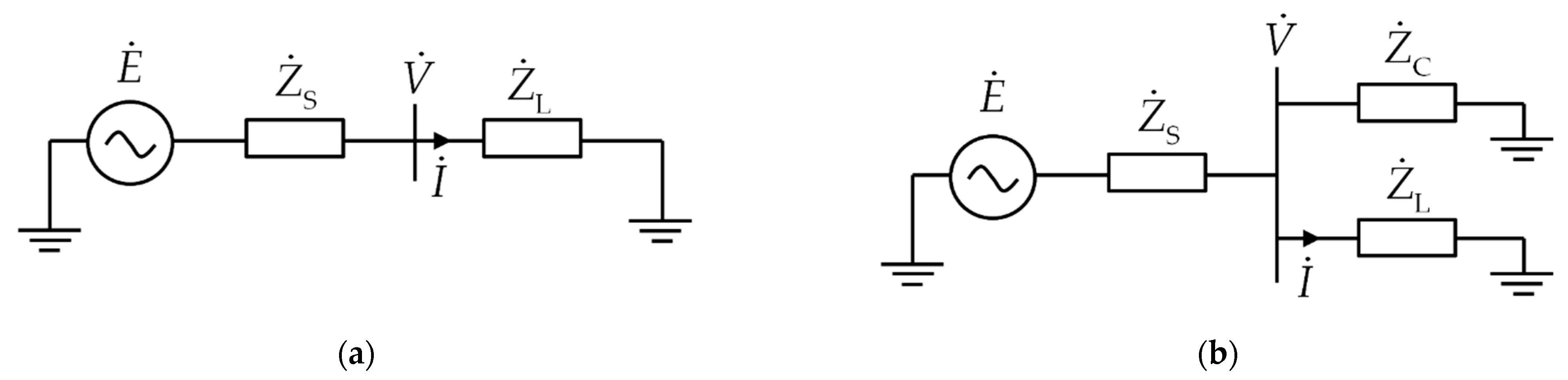
Testing of individual methods was performed using 2 simple power system models shown in
Figure 1 created by MATLAB script. In the case of both models, the constant power system impedance
= (0.5 + j4) Ω was considered. Within the power system model according to
Figure 1a, the line-to-line voltage value of the equivalent voltage source changed randomly in the interval of 118 kV ± 0.1 kV, and the load impedance
changed randomly in the interval of (300e
j23.1° ± 12) Ω (only resistive part) within the 1st quarter simulated data and in the interval (300e
j23.1° ± <−70; 9>) Ω (only resistive part) within the remaining three-quarters of the simulated data. In the case of the network model, according to
Figure 1b, the line-to-line voltage of the equivalent voltage source and load impedance changed randomly at the same intervals as in Case 1 (a), but in addition, the parallel load impedance
also changed randomly in the interval of (500e
j18.2° ± 12) Ω. The total number of samples generated in each simulation was 1e4.
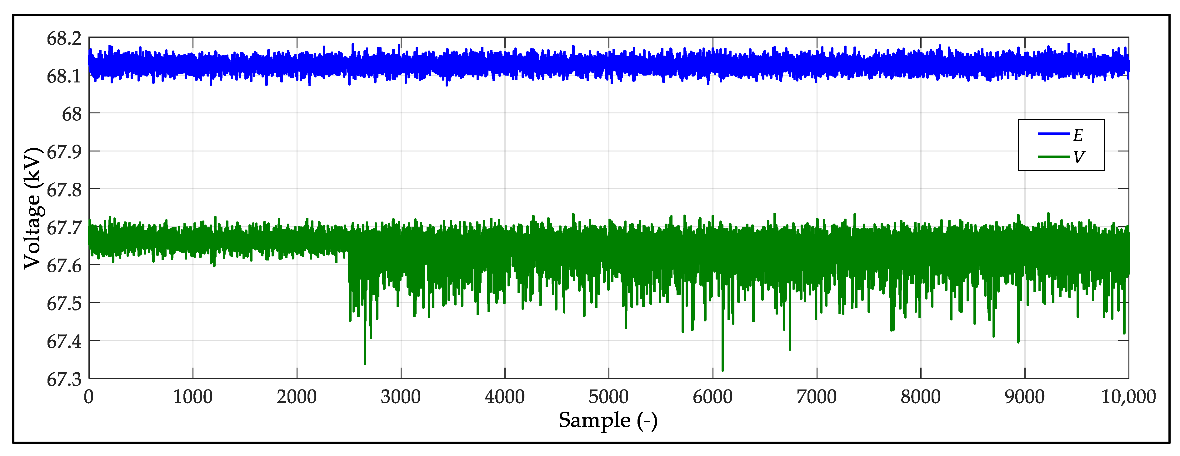
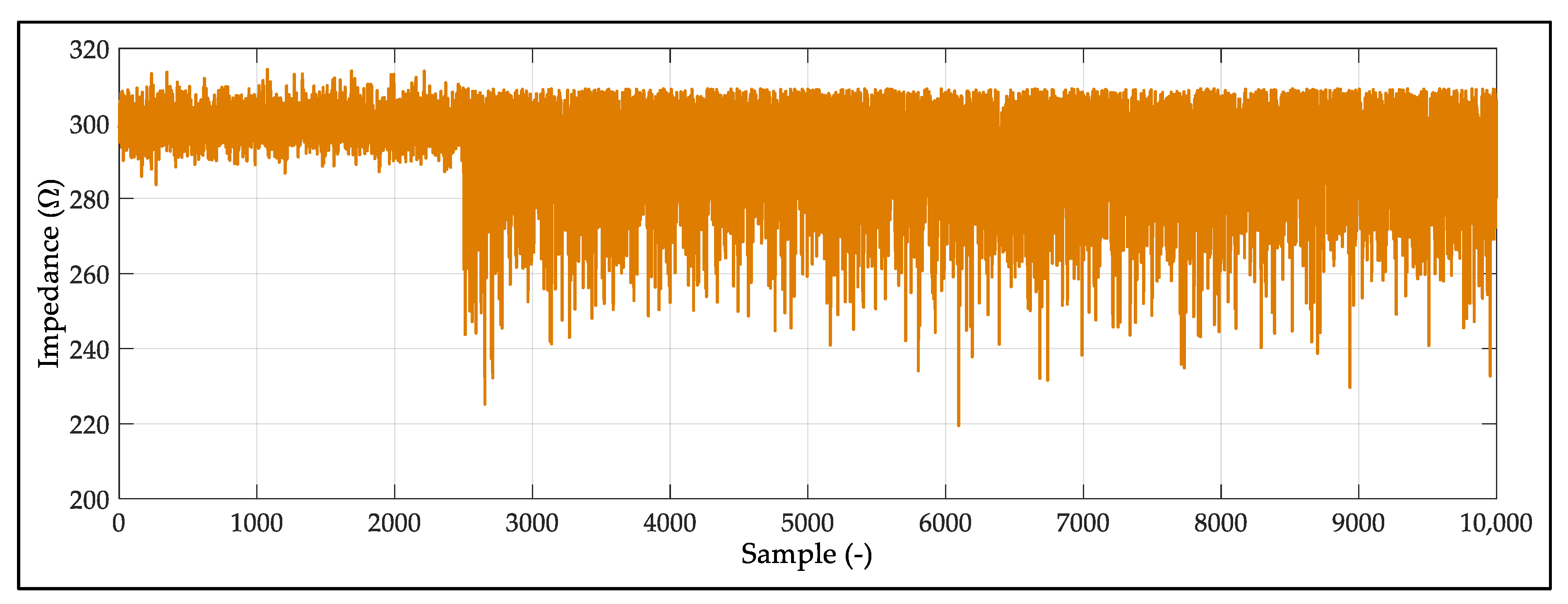
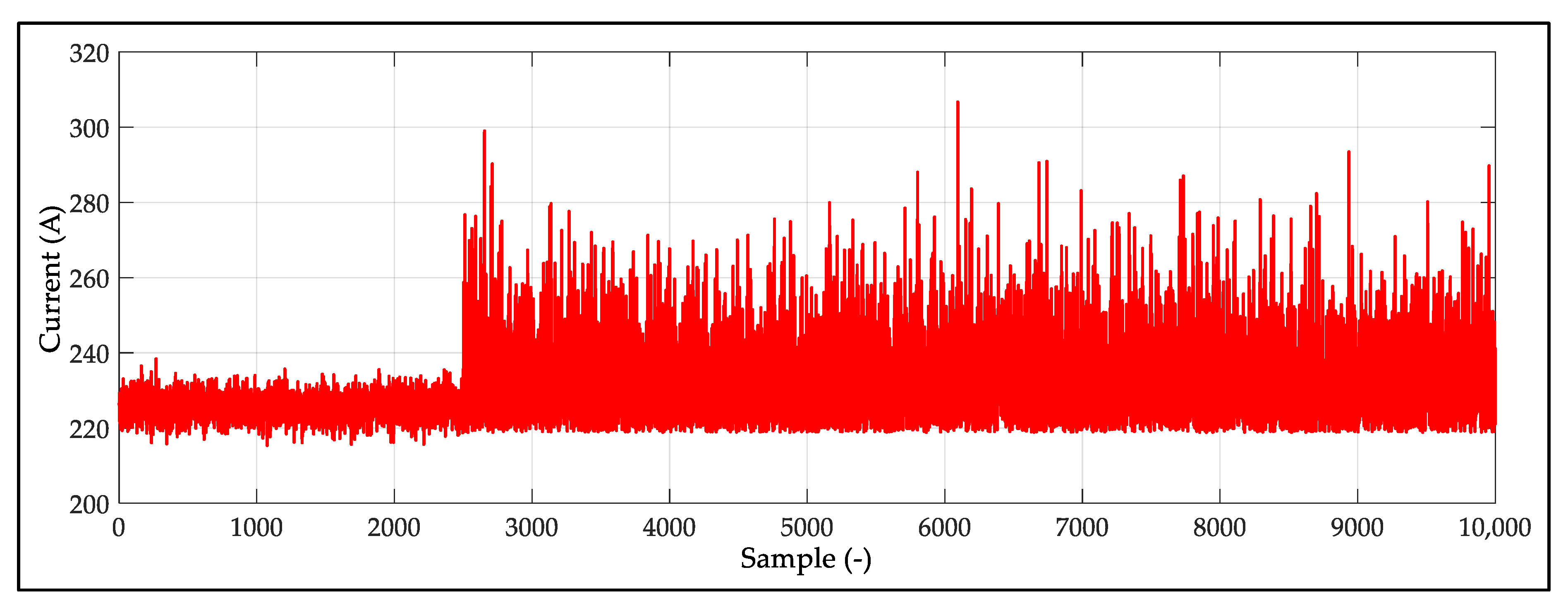
Figure 2,
Figure 3 and
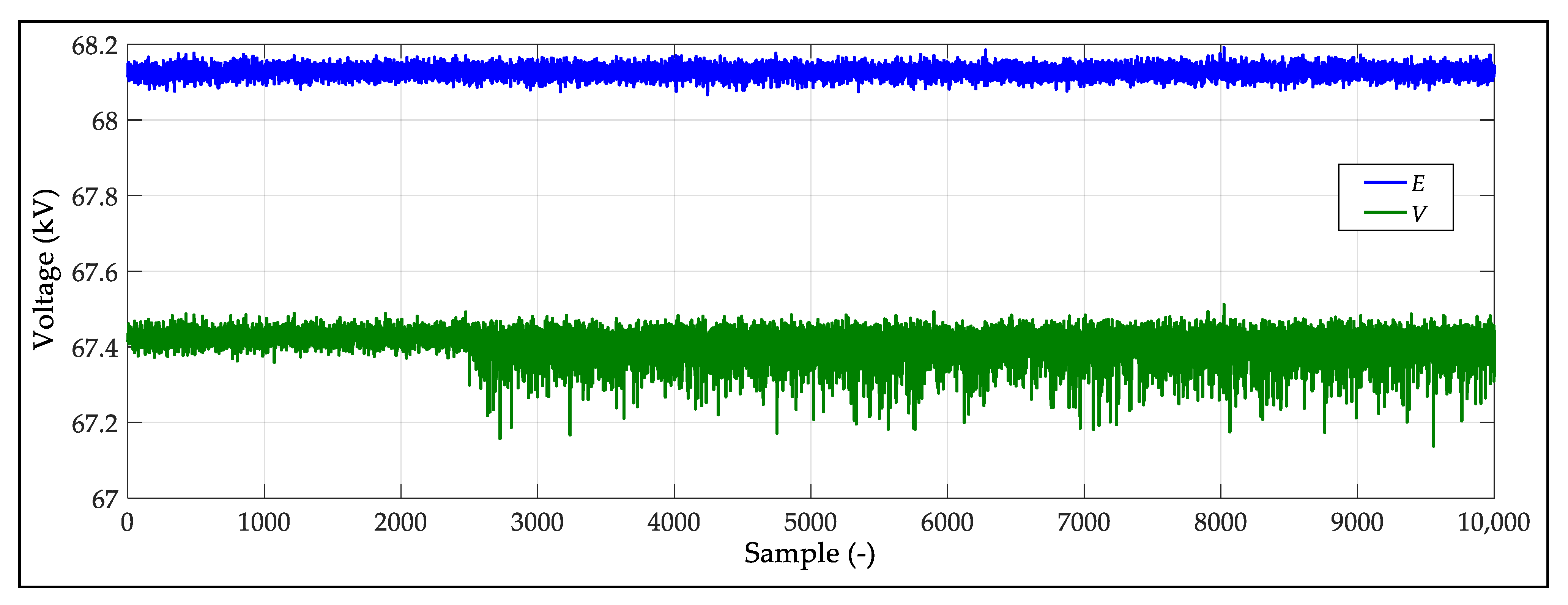
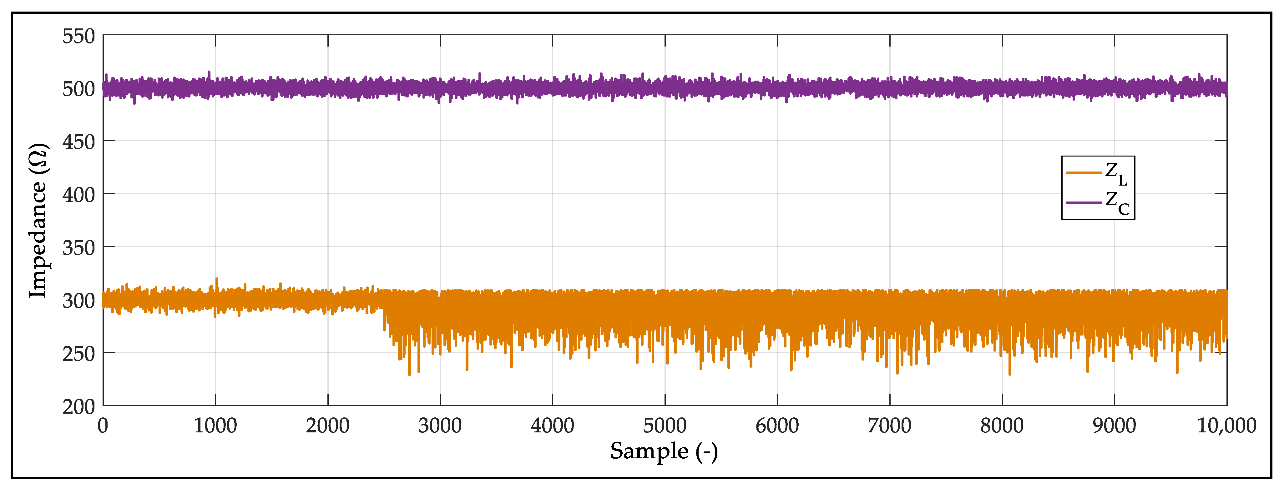
Figure 4 show the time courses of the RMS voltage, the load impedance, as well as the RMS current of load in the case of a simulation carried out using a model without considering a parallel load (according to
Figure 1a).
Figure 2 shows the variation of the RMS voltage of the voltage source and of the voltage at the load. From the 2500th sample, there was a more pronounced variation in the load impedance (see
Figure 3), which was reflected in an increase in the variation of the RMS voltage
V.
Table 1 shows the results of the evaluation of the power system impedance calculation using the individual methods applied by MATLAB script to the data shown in
Figure 2,
Figure 3 and
Figure 4. Among all considered the methods described in
Section 2, method No. 3 and method No. 6 were not applied for this analysis. In the case of method No. 3, the simulated data reached unrealistic results, probably due to the insufficient number of 3 consecutive samples with a constant value of load impedance. Determination of the power system impedance in the case of method No. 6 was based on analyzing the change in the negative sequence of the voltage and current, but the simulated data representing voltage and current changed only in a positive sequence. Calculation of the power system impedance using methods No. 1 to 5 was realized on the basis of the selection of 2500 samples with the largest current change. Only 1515 samples from selected 2500 samples met the criteria of the required impedance (
and
) in the case of method No. 5. In the case of method No. 7, all simulated samples were included in the calculation, but only 9 samples met the specified calculation criteria (
and
). As can be seen from the results in
Table 1, all the methods tested led to the determination of the power system impedance (not only the size but also the
ratio) with very good accuracy. The most accurate value of the power system impedance (set to value
= (0.5 + j4) Ω) from the evaluated data was determined by method No. 1, and the least accurate value was determined using method No. 7 (however, due to the final number of samples (9) entering the calculation, the accuracy of the resulting value was excellent).
Figure 5,
Figure 6 and
Figure 7 show the time courses of the RMS voltage, the load impedance as well as the RMS current of load in the case of a simulation carried out using a model considering a parallel load (according to
Figure 1b).
Figure 5 shows the variation of the RMS voltage of the voltage source as well as of the voltage at the load. In addition, in this case, there was a more significant fluctuation of the load impedance
from the sample of 2500 (see
Figure 6), which was reflected in an increase in the fluctuation of the RMS voltage
.
Table 2 shows the results of the evaluation of the power system impedance calculation using the individual methods applied to the data shown in
Figure 5,
Figure 6 and
Figure 7. Among all the considered methods described in
Section 2, also in this case method No. 3 and method No. 6 were not applied for this analysis due to the same reasons as in the previous case. Calculation of the power system impedance using methods No. 1 to 5 was realized on the basis of the selection of 2500 samples with the largest current change. Only 1458 samples from selected 2500 samples met the criteria of the required impedance (
and
) in the case of method No. 5. In the case of method No. 7, all simulated samples were included in the calculation, but only 11 samples met the specified calculation criteria (
and
). As can be seen from the results in
Table 2, even in this case all the methods tested led to the determination of the power system impedance (not only the size but also the
ratio) with very good accuracy (the value of power system impedance was set to
= (0.5 + j4) Ω in the model). The most accurate value of the power system impedance from the evaluated data was determined by method No. 1, 2, 4, and the least accurate value was determined using method No. 7 (however, due to the final number of samples (11) entering the calculation, the accuracy of the resulting value was excellent also in this case).
3.2. Real Measurement Test
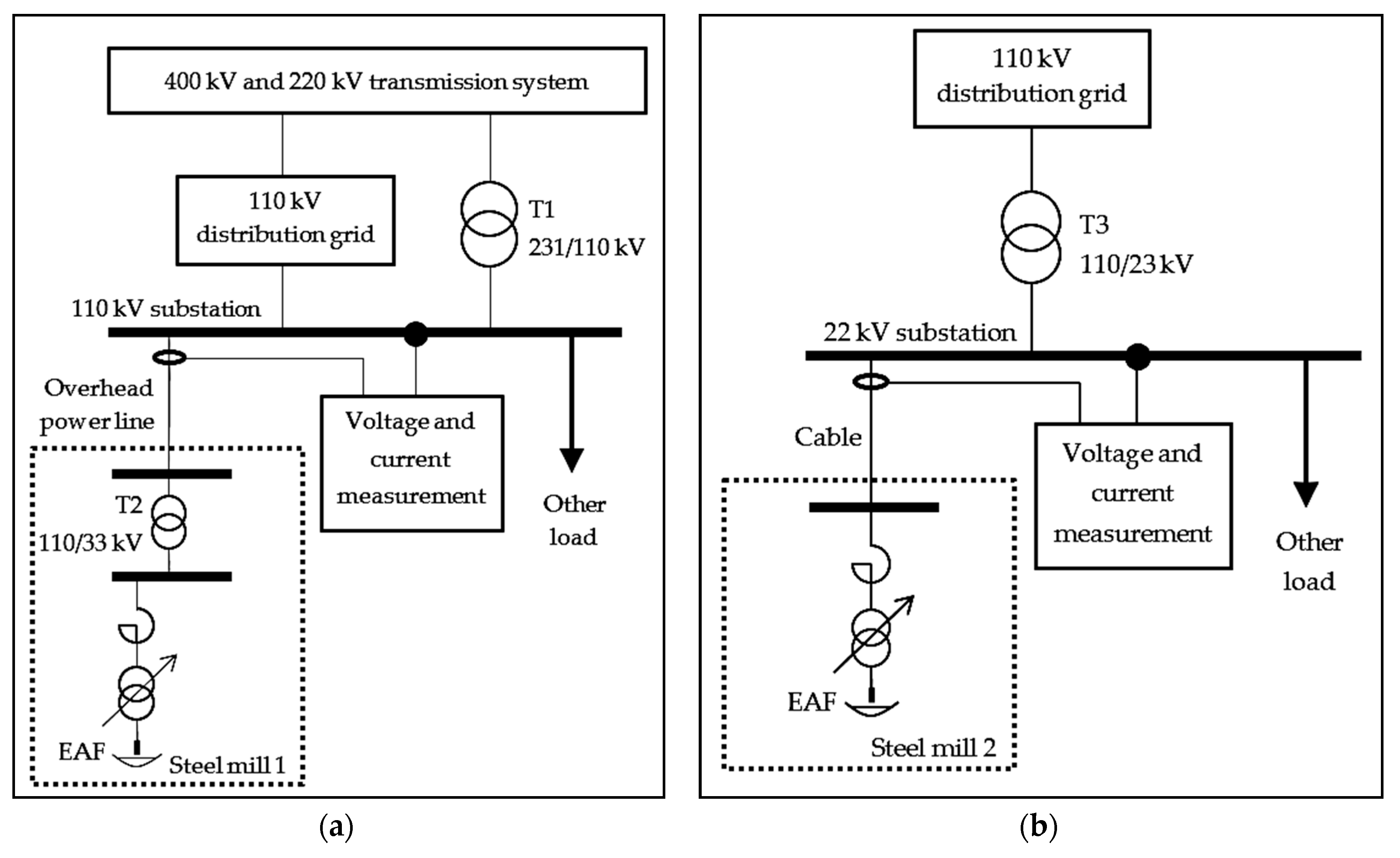
The application of individual methods for determining the power system impedance from real measured data was realized using 3 measurements of the time course of the RMS value and the angle of voltage and current in 110 kV, and at a 22 kV substation supplying a steel mill with an electric arc furnace (EAF) operation.
In the case of the first 2 measurements, it was the same measuring point (supplying the Steel mill 1), but under different conditions in the 110 kV distribution grid configuration. A single-line diagram for measurement No. 1 and 2 is shown in
Figure 8a. Based on information from the distribution system operator, the level of short-circuit power within the considered 110 kV substation, depending on the configuration of the power system and the operation of the sources, can range from 1000 MVA to 3700 MVA. According to the assumptions of the distribution system operator, the configuration of the power system at the time of measurement No. 1 led to the value of short-circuit power in the 110 kV substation to the level from 2800 MVA to 3200 MVA, which represents the value of the power system impedance in the interval 4.2 Ω to 4.8 Ω. Power system configuration at the time of measurement No. 2 led, according to the assumptions of the distribution system operator, to the value of short-circuit power in the 110 kV substation to the level from 1600 MVA to 1900 MVA, which represents the value of the network impedance in the interval 7.0 Ω to 8.3 Ω.
In the case of the 3rd measurement, it was a measuring point in the 22 kV substation, from which Steel mill 2, also with the operation of the arc furnace, was supplied. A single-line diagram for measurement No. 3 is shown in
Figure 8b. The 22 kV substation was supplied from the 110 kV distribution system only through one 110/23 kV transformer with a nominal power of 16 MVA, a short-circuit voltage of 10.7%, and nominal load losses of 77.5 W. The maximum value of short-circuit power on the 22 kV busbar of this substation was guaranteed at the level of 148 MVA, which represents a power system impedance of approximately 3.6 Ω. Since the positive sequence impedance of the transformer T3 represents a value of 3.48 Ω (according to Section 6.3 of IEC 60909-0: 2016), the measured value of the power system impedance should not fall below this value.
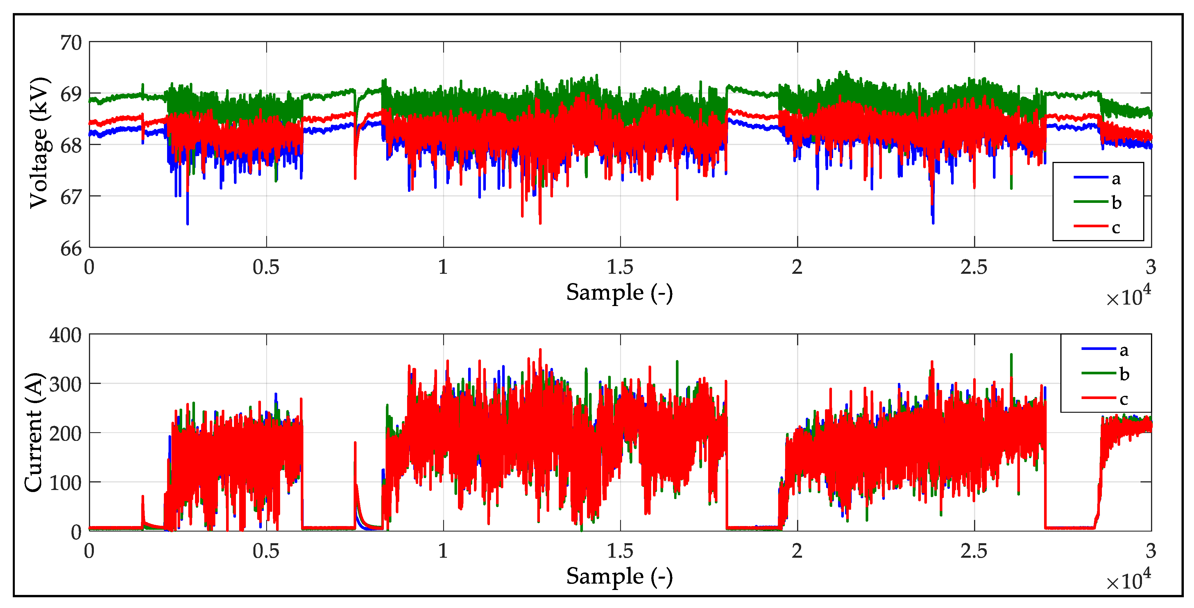
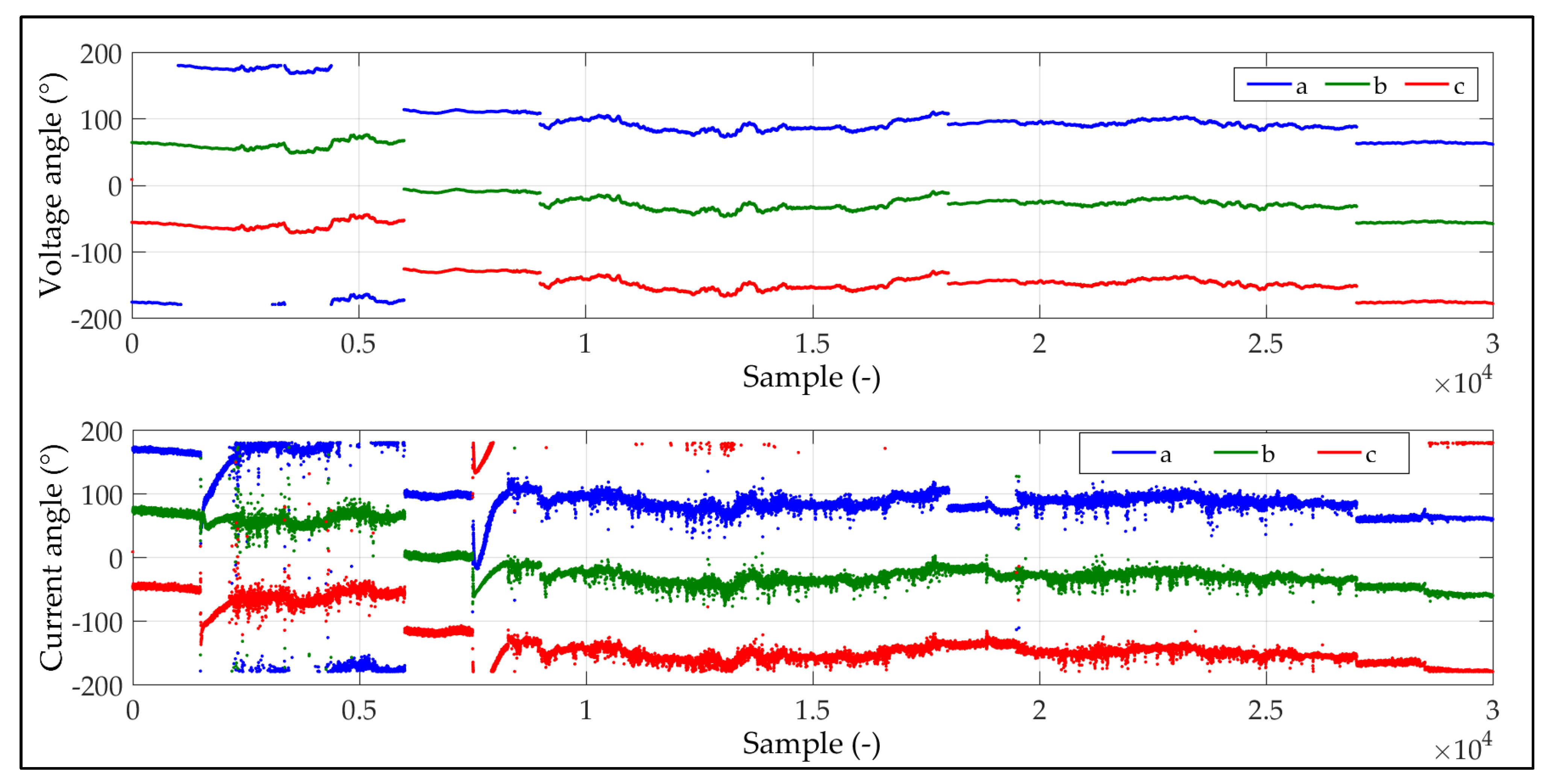
In the case of all 3 measurements, 10 min recordings of RMS values and angles of voltages and currents of the fundamental frequency (50 Hz) with a recording interval of 1 period (0.02 s) were performed. The total number of recorded and thus evaluated data was 30,000 samples for each measurement.
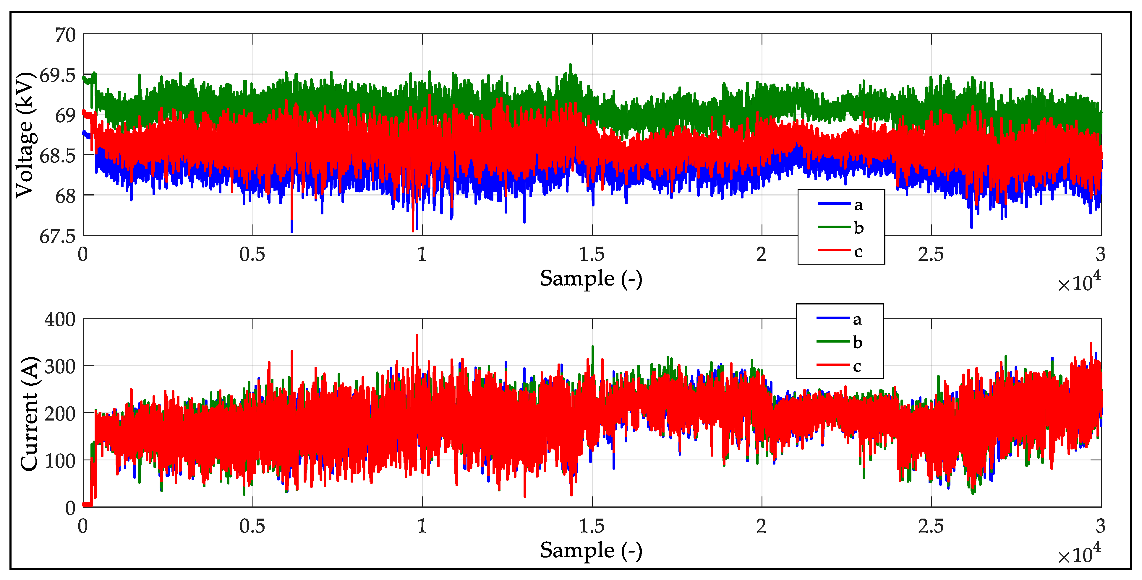
Figure 9 and
Figure 10 show the time courses of the RMS values of voltages and currents, or angles of voltages and currents in all 3 phases measured in measurement No. 1. Within the first 240 samples, it was possible to observe the magnitude of the voltage as well as the level of its fluctuation without the operation of the EAF (in
Figure 9). Subsequently, it was possible to observe the effect of the RMS current variation on the variation of the RMS voltage during the operation of the EAF.
Figure 11 and
Figure 12 show the time courses of the RMS values of voltages and currents, or angles of voltages and currents in all 3 phases measured in measurement No. 2. In this case, it was possible to observe the magnitude of the voltage as well as the level of its fluctuation without the operation of the EAF within 4 significant intervals (see
Figure 11). In addition, it can be seen in
Figure 11 the effect of fluctuations in RMS current on fluctuations in RMS voltage during EAF operation.
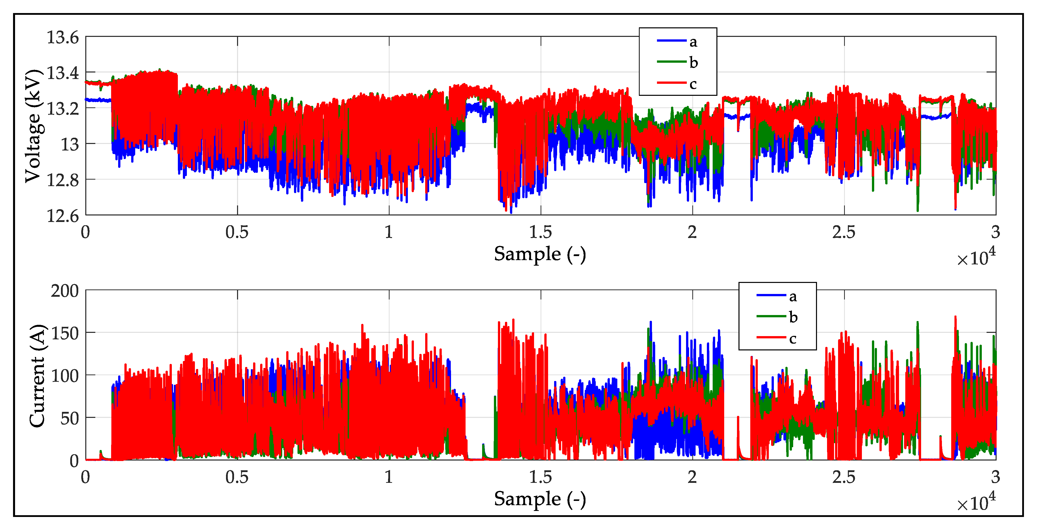
Figure 13 and
Figure 14 show the time courses of the RMS values of voltages and currents, or angles of voltages and currents in all 3 phases measured in measurement No. 3. In addition, in this case, it was possible to observe the magnitude of the voltage as well as the level of its fluctuation without the operation of the arc furnace within 4 more significant intervals (see
Figure 13), as well as the effect of fluctuations in RMS current on fluctuations in RMS voltage, can also be observed.
The evaluation of the power system impedance was performed using all 7 considered methods from the measured data. Methods No. 3 and No. 7 were designed to consider only data meeting the assumptions of these methods from the whole data set. In the case of other methods, only samples corresponding to 2500 of the largest step changes in the RMS value of the positive sequence current were considered for the power system impedance evaluation. Because method No. 6 was designed to evaluate power system impedance based on step changes of the negative sequence voltages and currents, we applied this method for 2 different sets of 2500 samples. The 1st set of 2500 samples was the same as for the other methods (i.e., corresponding to 2500 of the largest step changes in the RMS value of the positive sequence current), and we labeled this approach as 6a. The 2nd set of 2500 samples was corresponding to 2500 of the largest step changes in the RMS value of the negative sequence current, and we labeled this approach as 6b.
Table 3 shows the final numbers of samples from which the power system impedance calculations were performed by individual methods in the case of measurements No. 1 to 3. Subsequently,
Table 4,
Table 5 and
Table 6 show the results of the calculations of resistance (
RS), reactance (
XS), and the magnitude of the total power system impedance (
ZS) calculated for each measurement using the individual methods. Asterisks (*) in these tables indicate values that did not meet the assumptions or represent an unrealistic value.
The results of the power system impedance determined by individual methods in the case of 3 sets of real measured data presented in this article show their greater ambiguity, as it was in the case of their application to simulated data (described in
Section 1).
In the case of measurement No. 1, it was possible to observe the results of the calculation within the expected interval (4.2 Ω to 4.8 Ω) within methods No. 1 to 5. However, even in the case of methods No. 6 and 7, a realistic value was determined. A possible reason for a larger deviation of the calculated value of the power system impedance from other methods in the case of method No. 6 was the fact that this method was based on the assessment of the change in the negative sequence of voltage and current, while the samples selected for analysis has been selected on the basis of the largest positive sequence current changes. In the case of method No. 7, it met the specified calculation criteria ( and ) with only 19 samples, which was relatively small out of the total number of 30,000 samples.
Measurement No. 2 pointed out a more fundamental problem in the application of methods No. 3 and 4 for a given data set. In these 2 cases, too high values of the power system impedance, and in the case of method No. 4, negative power system reactance values were calculated. Other methods led to the calculation of the realistic value of the power system impedance, although the results of the calculation obtained using methods No. 2 and 6 were more pronounced than the expected value.
Measurement No. 3 was realized in a substation, within which it was clear that the magnitude of the power system impedance could not be less than 3.48 Ω and at the same time, it was not assumed that the value of 4.8 Ω should not be exceeded. In this case, the expected results were obtained using methods No. 1, 5, and 6, although in the case of method No. 1, a negative network resistance value was determined. Since this value was close to 0, it can be assumed that this was a certain statistical deviation within the selected data set. Although impedance values obtained by methods No. 3 and 7 represented a realistic value, they moved more significantly from the expected result. Methods No. 2 and 4 completely failed in this case.
Among the analyzed methods, methods No. 1 and No. 5 seemed to be the most suitable for power system impedance estimation based on fast voltage and current changes measurements. Nevertheless, based on the obtained results, it is not possible to say unequivocally that these 2 methods are more suitable or less suitable for determining the power system impedance within a wide range of measured data. In this context, it should be emphasized that the individual methods have been applied to a specific type of data measured during the operation of EAF. Methods No. 3 and 7 were designed to determine the power system impedance within the standard steady-state operation, within which, for example, it would not be possible to apply method No 5.


