A Short-Term Residential Load Forecasting Model Based on LSTM Recurrent Neural Network Considering Weather Features

Abstract

With economic growth, the demand for power systems is increasingly large. Short-term load forecasting (STLF) becomes an indispensable factor to enhance the application of a smart grid (SG). Other than forecasting aggregated residential loads in a large scale, it is still an urgent problem to improve the accuracy of power load forecasting for individual energy users due to high volatility and uncertainty. However, as an important variable that affects the power consumption pattern, the influence of weather factors on residential load prediction is rarely studied. In this paper, we review the related research of power load forecasting and introduce a short-term residential load forecasting model based on a long short-term memory (LSTM) recurrent neural network with weather features as an input.

1. Introduction

With the progress of technology and the development of society, the energy supply, especially the electricity supply, plays an increasingly important role in economic activities and daily life. Due to the synchronization of the power generation, transmission and utilization processes combined with the inability to store large quantities of electric energy, a reasonable power dispatching scheme needs to be formulated in order to guarantee the stability and economy of the power system operation. Therefore, power load prediction plays a very important role in the process of the transition toward a more intelligent and more refined power system.

From the perspective of forecasting step size, power load forecasting can be divided into long-term, mid-term and short-term. Long-term forecasting with the target to forecast annual and monthly loads is usually used in power infrastructure construction planning while medium-short-term forecasting, which forecasts weekly, daily and hourly power loads, plays an important role in the system operation.

With the increasing diversification of the production method and lifestyle, an accurate short-term load prediction on a residential level can greatly promote the operation of the power system. To integrate the increasing volume of intermittent renewable generation into modern power grids, integrators are exploring ways to manipulate residential and commercial loads in real-time [1]. Therefore, various demand response (DR) frameworks that can shape power demand by broadcasting time-varying signals to customers are becoming more and more popular. Accurate real-time prediction of energy demand of users is helpful for power suppliers to understand user demand and formulate more reasonable and efficient DR projects. Forecasting load demand is of great significance to power system capacity planning and future investment.

However, as the residential power load is inevitably affected by the weather, holidays, electricity prices, lifestyle and other factors, short-term power load forecasting on a residential level is still a difficult and challenging problem.

This paper studies the relation between weather features and residential loads and introduces a short-term residential load forecasting model based on an LSTM recurrent neural network to verify the assumption. Section 2 introduces the existing power load forecasting methods, the problems and challenges and the necessity to study the influence of weather characteristics on the short-term power load. Section 3 analyzes the weather characteristics of the dataset and presents the relation between different weather features and the residential load. Section 4 introduces the workflow of the proposed model based on LSTM. Section 5 shows the performance of the model on the power load dataset.

2. Previous Work

One-day-ahead forecasting of aggregated power loads has been widely studied in previous works. Different approaches have been proposed to solve the issue. Statistical methods include a time series analysis [1,2,3,4] and a regression analysis [5,6,7] but the forecasting results lack accuracy. With the development of machine learning research, technologies such as the neural network [8,9] and the support vector machine [10,11] are gradually introduced into the daily load forecasting model of power systems. Ghofrani et al. [12] proposed a dedicated input selection scheme to work with the hybrid forecasting framework using wavelet transformation and a Bayesian neural network. Duong-Ngoc et al. [13] studied the correlation between a feedforward deep neural network (FF-DNN) and a recursive deep neural network (R-DNN) and combined the two deep neural network architectures for a power load forecasting task in Ho Chi Minh City. Among all of the literature studied, this approach achieved the most accurate forecasting performance on system level load forecasting with a mean absolute percentage error (MAPE) as small as 0.350% on average. In addition, the work of Zhang et al. [14] also shows the potential of a deep residual network (ResNet) to improve power load forecasting by mitigating gradient vanishing and explosion problems.

The studies above take historical data as the input feature and a few add workday/holiday features into the input matrix. However, in addition to historical patterns and workday/holiday features, weather is also an important factor that affects power load. In past studies, many researchers have taken weather data into account. In [15], an artificial neural network (ANN) and bagged regression trees were developed to generate a load forecast in Sydney/New South Wales using temperature data. In [16], mutual information (MI) was used as the index to select input features. The correlation between temperature, irradiance and load was analyzed. By selecting the input features through MI, the accuracy of the ANN model was improved. In [17], the Humidex Index, a comprehensive index of atmospheric temperature and humidity as an input to forecast the regional power load of a small town in Italy with the special feature that there were only household users in the region without commercial and industrial users, was used. Compared with previous studies using single weather data, this study uses comprehensive weather indicators and the results show that the addition of weather indicators can greatly improve the prediction performance of an ANN.

All of the above methods focus on learning and forecasting the load at the system or substation level. With the appearance of smart meters and the development of automatic meter reading (AMR) technology, the short-term load prediction on residential level has gradually become the focus of researchers. In the existing literature, the work of Ghofrani et al. [18] was the first to focus on the prediction of individual user load. They studied the potential impact of AMR on short-term load forecasting for residential users. The results show that the availability of more real-time measurement data greatly improves the accuracy of load forecasting but computational complexity will increase dramatically at the same time. In recent years, deep learning has gained increasing attention in the field of short-term power load forecasting for individual users. In [19], a hybrid model with an extreme learning machine and an extended Kalman filter for online short-term load prediction was proposed. However, although focusing on micro-grid research, the data obtained by smart meters in 2014 are still not detailed to every household. The dataset used in this study is relatively small, only including the hourly load data of two residential buildings and two commercial buildings. In [20], a framework based on an LSTM recurrent neural network to forecast the residential load of 69 customers was proposed and MAPE was used to compare this with various benchmarks including state-of-the-art load forecasting and achieved satisfactory results but the researchers selected the data by pre-screening the users, which may have affected the results. Afrasiabi et al. [21] proposed a direct prediction model of the conditional probability density of a residential load based on a deep hybrid network. It achieved high accuracy in both the prediction of a single household’s power load and the prediction of an aggregated load of 3500 residential households. All studies mentioned above only used historical data as model input characteristics without considering the influence of weather factors on a single-family load.

Currently there is little research focused on micro-grid power load forecasting considering weather factors; [22] aimed to provide a day-ahead residential load prediction and directly used the outdoor air temperature as the weather characteristic but did not explore the specific influence of different weather characteristics. Our paper aims to study the influence of meteorological data on a single household power load and provide an hour-ahead load forecast. Firstly, the correlation between the load data and the weather characteristics is measured by calculating the standardized cross-correlation value then we choose the most relevant one or two meteorological features as the input. The hour-ahead prediction is carried out through an LSTM network.

3. Feature Selection

Unlike a regional integrated power load, which has more regular hourly, daily and weekly seasonality, a residential power load is more affected by the exogenous variables such as the lifestyle of the residents, behavior rules and the response to the weather changes so there is a stronger irregularity.

The dataset used in this study is the UMass Smart* Dataset released in 2017 [23]. The apartment dataset contains data obtained from 114 single-family apartments including the apartment’s per-minute electrical load and hourly meteorological data (temperature, humidity, pressure, apparent temperature, wind speed, etc.).

In this section, the correlation between various weather features and the load is evaluated through the cross-correlation value. The factor with the strongest correlation is then selected as the input to the prediction model. Finally, the distribution of the selected indexes in all of the years is analyzed to provide a basis for dividing the training set and the test set.

3.1. Normalized Cross-Correlation

The cross-correlation function represents the correlation between two time series; that is, it describes the correlation between the values of signals x(t) and y(t) at any two different moments, T1 and T2. For discrete time series, the cross-correlation function can be defined as follows:

$$cross\_corr\left(x,y\right)={\displaystyle \sum }_{i=0}^{n-1}{x}_i\times y_i.$$

(1)

There are three problems when using a cross-correlation value to evaluate the correlation:

• The score value of the cross-correlation is difficult to understand.
• Both sequences must be of the same magnitude. If a sequence value is reduced by half, its relevance is reduced.
• Inability to solve the problem of a sequence value of 0.

To solve these problems, a standardized cross-correlation function is used:

$$norm\_cross\_corr\left(x,y\right)=\frac{{{\displaystyle \sum }}_{i=0}^{n-1}{x}_i\times y_i}{\sqrt{{{\displaystyle \sum }}_{i=0}^{n-1}{x}_i{}^2\times {{\displaystyle \sum }}_{i=0}^{n-1}{y}_i{}^2}}.$$

(2)

The cross-correlation values after standardization have the following characteristics:

• The higher the absolute value, the higher the correlation. When two signals are exactly the same, the maximum value is 1; when the two signals are completely opposite, the minimum value is −1.
• The correlation of time series with different amplitudes can be detected.

3.2. Results

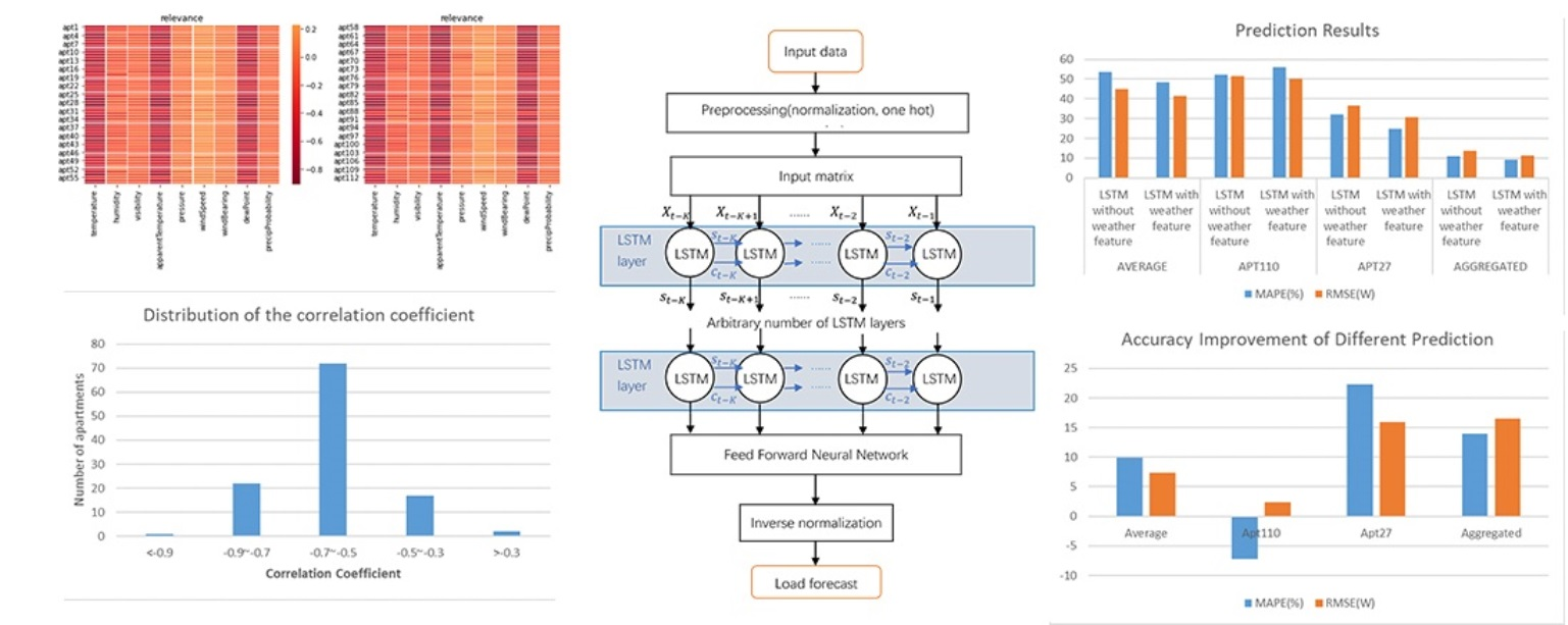
In this study, the weather dataset contained features such as ’temperature’, ‘humidity’, ‘visibility’, ‘apparent temperature’, ‘pressure’, ‘wind speed’, ‘wind bearing’, ‘dew point’ and ‘probability of precipitation‘. We conducted a correlation analysis on these indicators and the load data at the same time and the results are shown in Figure 1.

As shown vividly in Figure 1, the temperature, apparent temperature and dew point were the most relevant factors corresponding with residential power load and all three variables were correlated with temperature. The temperature generally refers to air temperature; dew point refers to the temperature at which gaseous water contained in air reaches a saturation point and condenses into liquid water at a fixed pressure; apparent temperature refers to the degree of warmth and coldness felt by human body, which is influenced by air temperature, wind speed and relative humidity [24]. It is calculated by Equation (3):

$$AT=1.07T+0.2e-0.65V-2.7,$$

(3)

where AT is body temperature (°C), T is air temperature (°C), e is water vapor pressure (hPa), V is wind speed (m/SEC).

As the three variables with the highest correlation were all related to temperature and as apparent temperature was the most comprehensive factor among the three variables, we only chose apparent temperature as the meteorological input feature for the short-term load prediction.

By analyzing the specific data, it was found that the correlation coefficient between apparent temperature and load ranged from −0.22 to −0.9. The specific data distribution is shown in

Table 1. Distribution of the correlation coefficient.

Correlation Coefficient	<−0.9	−0.9 ~ −0.7	−0.7 ~ −0.5	−0.5 ~ −0.3	>−0.3
Number of Apartments	1	22	72	17	2
Percentage (%)	0.88	19.30	63.16	14.91	1.75

and Figure 2. A total of 83.34% of the tested apartments had a correlation that was greater than 0.5 and only 19 apartments had a relatively low correlation, which was consistent with common sense in reality. The electricity consumption patterns of most people are affected by temperature and the magnitude of the influence is determined by the different sensitivity of people towards temperature change. A few people are not sensitive to climate change so the electricity consumption patterns are less affected by temperature.

3.3. The Distribution of Apparent Temperature

Due to privacy protection and other issues, the organization that published the dataset did not give detailed information of the tested users (location, consumption pattern, etc.) so in order to understand the weather characteristics of the test site, we visualized the annual distribution of the apparent temperature in Figure 3.

Through the analysis of the weather data from 2014 to 2016, we found that the meteorological data of November and December were similar to that of March, April and May and the obvious cold season occurred in January and February. This was a great help for us to divide the training set from the test set; by using data from the first nine months as the training set, the model could learn about changes in the patterns of electricity consumption in all weather conditions.

4. STLF Model

4.1. LSTM

A long short-term memory network (LSTM) is a type of temporal cyclic neural network [25], which is specially designed to solve the long-term dependency problem existing in a general RNN (recurrent neural network). In an LSTM network, the hidden layer neurons of a traditional RNN network are replaced with memory units. The structure of the memory unit, which includes input gate, forgetting gate and output gate, can make the network delete invalid information or retain important information at each time step.

In many fields such as language translation and speech recognition, an LSTM recurrent network has become one of the ideal candidate networks due to its ability to learn temporal correlations. Such temporal correlations are widely spread in the electricity consumption of individual households because they are based on the behavior of the residents, which is difficult to learn and predict. In the case of residential load prediction, the LSTM network is expected to extract the states of the residents from the pattern of the input power consumption profile, then keep the memory of these states and finally make the prediction according to the learnt information [20].

The structure of an LSTM cell block is shown in Figure 4.

The calculation process is shown in Equations (4)–(9).

$$f_t=\sigma \left(W_f\left[s_{t-1},x_t\right]+b_f\right),$$

(4)

$$i_t=\sigma \left(W_i\left[s_{t-1},x_t\right]+b_i\right),$$

(5)

$${\tilde{C}}_t=tanh\left(W_c\left[s_{t-1},x_t\right]+b_c\right),$$

(6)

$$C_t=f_t{C}_{t-1}+i_t{\tilde{C}}_t,$$

(7)

$$o_t=\sigma \left(W_o\left[s_{t-1},x_t\right]+b_o\right),$$

(8)

$$s_t=o_{t}tanh\left(C_t\right).$$

(9)

The forget gate $f_t$ is first calculated, which determines how much information the current memory cell has forgotten from the previous cell state $C_{t-1}$. The current input $x_t$ combined with the previous hidden state $s_{t-1}$ is used as the input to the memory cell. $W_f$ is the weight matrix of the forget gate. The input gate $i_t$ determines how much information from the input signal can be sent into the global cell state. $W_i$ is the weight matrix of the input gate. The current cell state ${\tilde{C}}_t$ is then calculated and the global cell state $C_t$ is updated according to the input gate and the forget gate. Finally, the output state $s_t$ at the current moment is determined by the output gate $o_t$. $b$ is the bias for every gate.

4.2. STLF Model Based on LSTM

The short-term forecasting framework based on LSTM is shown in Figure 5.

The framework starts with the preprocessing of the input data. In this study, the following input features were used:

• The sequence of the power load in the past K time steps: $ℒ=\left\{l_{t-K},\dots ,l_{t-2},l_{t-1}\right\}ϵ{ℝ}^K$.
• The sequence of the last-week power load for the past K time steps: ${ℒ}_w=\left\{l_{w-K},\dots ,l_{w-2},l_{w-1}\right\}ϵ{ℝ}^K$.
• The weather feature sequence for the K time steps:$Tϵ{ℝ}^K$.
• The corresponding binary holiday marks $H$ where $H=0$ when it was a working day and 1 when it was not.

As LSTM is sensitive to the data scale, the four input vectors were scaled to the range of (0, 1) according to the nature of the feature. The minimum-maximum normalization was applied on $ℒ$, ${ℒ}_w$ and $T$ while $H$ was encoded by one hot encoder.

After the four vectors were scaled to $\widetilde{ℒ,} \widetilde{{ℒ}_w},\widetilde{T,} \tilde{H}$, the input matrix for the LSTM model was given as:

$$X=\left[{\widetilde{ℒ}}^{\mathrm{T}},{\widetilde{{ℒ}_w}}^{\mathrm{T}},{\tilde{T}}^{\mathrm{T}},{\tilde{H}}^{\mathrm{T}}\right].$$

(10)

Each row referred to the input eigenvector of the corresponding time step.

An Adam optimization algorithm proposed by Kingma et al. [26] was adopted in the model training process in this paper. The traditional gradient descent method, no matter whether it is single sample processing or batch sample processing, cannot reach a good balance between the training time and calculation precision. However, the Adam optimization algorithm has the characteristics of less consumption of storage resources, a short training time, a high computation efficiency, fewer hyperparameters and the ability to deal with non-stationary targets so that the model could converge to a relatively ideal state accurately and quickly. The experimental results showed that the Adam algorithm outperformed the root mean square prop (RMSProp), adaptive gradient (AdaGrad), AdaDelta and other commonly used optimization methods in the training effect.

5. Results and Discussion

5.1. Test Settings

As is shown in Figure 6, the data of electricity consumption remained 0 for a long time in 2014 and suddenly showed an abnormally large and sharp increase at the end of 2015, which had a great adverse impact on the accuracy of prediction. Data from 2016 showed a better consistency and regularity; therefore, we only used the one-year data from 1 January 2016 to 31 December 2016 for training and prediction.

As the sampling interval of the smart meter in this project varied from 1 min to an hour, we integrated the data into the power load data of 1 h in order to maintain consistency with the sampling interval. This also coincided with the 1 h sampling interval for the weather data.

The period lasted for 365 days. According to different purposes, the data were divided into two subsets; namely, the training set (from 1 January 2016 to 19 October 2016) and the test set (20 October 2016 to 31 December 2016). The training set contained 292 days of data and the test set contained 73 days of data. The ratio of the training set to the test set was 0.8:0.2. The training set was used to train the prediction model and the test set was used to evaluate the results.

In general, hyperparameter tuning is a vast topic, which is essential for obtaining the best predictive performance. However, tuning the parameters of each individual model would have been time-consuming for this proof-of-concept paper as we were making separate predictions for 114 households. In this work, we only focused on verifying the influence of different weather features on the forecast results. Therefore, we chose commonly used two hidden layers and 20 memory units in each layer to build the model and set the timestep = 1, epochs = 15 and batch size = 144; therefore, the input matrix was a 1 × 4 matrix.

The root mean square error (RMSE) and mean absolute percentage error (MAPE) were used to estimate the accuracy of the forecast results. The formulae for RMSE and MAPE are as follows:

$$\mathrm{RMSE}=\sqrt{\frac{1}{n}{\displaystyle \sum }_{i=1}^n{\left({\widehat{x}}_i-x_i\right)}^2},$$

(11)

$$\mathrm{MAPE}=\frac{1}{n}{\displaystyle \sum }_{i=1}^n\left|\frac{\widehat{x_i}-x_i}{x_i}\right|\times 100\%,$$

(12)

where $\widehat{x}=\left\{\widehat{x_1},\widehat{x_2}, \dots \widehat{,x_n}\right\}.$ is the output of the forecasting model, $\mathrm{x}=\left\{x_1,x_2, \dots ,x_n\right\}$ is the actual value corresponding to the forecasting result and n is the number of the output.

5.2. Experimental Results and Discussion

Forecasting speed is very important for short-time power load forecasting. The proposed LSTM framework had the advantages of easy implementation, a strong portability and a short prediction time. All frameworks for all customers were built on a desktop PC with a 1.8 GHz AMD A8 processor and 4 GB of memory. For a single household, the time from the input of historical data to the generation of the prediction result was only 87.73 s on average. If predictions were carried out after model training, the average time for one prediction was only 6.65 s.

In order to verify the influence of weather factors on the prediction accuracy of a single household power load, we used different input features to forecast the single household power load. The prediction results are shown in

Table 2. Prediction results.

	MAPE (%)	RMSE (W)
LSTM without a weather feature	53.77	44.84
LSTM with a weather feature	48.46	41.51
Accuracy improvement (%)	9.87	7.43

.

It can be seen that adding weather features as part of the input matrix could effectively improve the accuracy of the load prediction.

Figure 7 and Figure 8 show the results of the power load forecast for the two apartments with the weakest and strongest correlations. Their numerical results are shown in

Table 3. Numerical results of Apartment 110.

	MAPE (%)	RMSE (W)
LSTM without a weather feature	52.19	51.36
LSTM with a weather feature	55.95	50.10
Accuracy improvement (%)	−7.20	2.45

and

Table 4. Numerical results of Apartment 27.

	MAPE (%)	RMSE (W)
LSTM without a weather feature	32.08	36.75
LSTM with a weather feature	24.92	30.88
Accuracy improvement (%)	22.32	15.97

.

It can be seen that in Apartment 110 with the weakest correlation between weather features and load, the addition of weather features did not contribute to improving the prediction accuracy but reduced the prediction accuracy to a certain extent. On the contrary, in Apartment 27, the two indexes of prediction accuracy were greatly improved after the addition of weather features.

When the hourly load of 114 apartments were summed up and combined into the electric load of an apartment building, which also belonged to a micro-grid, the forecast results and accuracy measurement are shown in

Table 5. Numerical results of the aggregated building.

	MAPE (%)	RMSE (W)
LSTM without a weather feature	10.95	1375.87
LSTM with a weather feature	9.42	1148.94
Accuracy improvement (%)	13.97	16.49

.

The above prediction results are summarized in Figure 9 and Figure 10.

It can be seen that after aggregating the 114 apartments’ load as a residential building, the forecast had a larger accuracy improvement (13.97% in MAPE and 16.49 W in RMSE) than the average of the individual forecast (9.87% in MAPE and 7.43 W in RMSE) and a smaller accuracy improvement than the forecast result of Apartment 27 (22.32% in MAPE and 15.97 W in RMSE). This made sense because the correlation between the weather characteristics and the electricity consumption patterns of all users was averaged after the integration. This strongly indicated that the addition of weather features could significantly improve the load prediction of either a single household or a whole building.

6. Conclusions

This paper attempted to explore the influence of weather characteristics on a single household electricity load prediction. Firstly, the correlation between the single household load and various weather characteristics was studied by calculating the cross-correlation value and the weather factors with the strongest correlation were obtained. According to practice theory, no matter how different residents’ lifestyles were, there were always repeated electricity consumption patterns [19]. Therefore, we chose LSTM as a prediction model for the single-family apartment load because LSTM has demonstrated the potential to learn repetitive patterns over a long period of time.

By analyzing 114 apartment users and the integrated building, the results showed that the addition of weather data had a positive effect on improving the prediction accuracy of most users but it might have a negative effect on users insensitive to weather changes. Overall, the impact of adding weather data was positive. The prediction of the whole building data also showed that the weather data had a positive effect on the improvement of the prediction accuracy of the aggregated data. This is of great significance to both regional load forecasting and residential load forecasting because most short-term power load forecasting studies on a residential level use only historical data and do not take weather into account.

As for future work, methods for parameter optimization can be developed to further improve the forecasting accuracy for different types of customers. It is also possible to explore the choice of input frames to reduce the negative impact of weather characteristics while forecasting the power load of weather-insensitive customers.

References

- Tucker, N.; Moradipari, A.; Alizadeh, M. Constrained Thompson Sampling for Real-Time Electricity Pricing With Grid Reliability Constraints. IEEE Trans. Smart Grid 2020, 11, 4971–4983. [Google Scholar] [CrossRef]
- Espinoza, M.; Joye, C.; Belmans, R.; Moor, B.D. Short-Term Load Forecasting, Profile Identification, and Customer Segmentation: A Methodology Based on Periodic Time Series. IEEE Trans. Power Syst. 2005, 20, 1622–1630. [Google Scholar] [CrossRef]
- Sfetsos, A.; Siriopoulos, C. Time Series Forecasting of Averaged Data with Efficient Use of Information. IEEE Trans. Syst. Man Cybern. Part A Syst. Hum. 2005, 35, 738–745. [Google Scholar] [CrossRef]
- Deb, C.; Zhang, F.; Yang, J.; Lee, S.E.; Shah, K.W. A review on time series forecasting techniques for building energy consumption. Renew. Sustain. Energy Rev. 2017, 74, 902–924. [Google Scholar] [CrossRef]
- Fan, S.; Methaprayoon, K.; Lee, W.J. Multi-area load forecasting for system with large geographical area. In Proceedings of the 2008 IEEE/IAS Industrial and Commercial Power Systems Technical Conference, Clearwater Beach, FL, USA, 4–8 May 2008. [Google Scholar]
- Tang, J.J.; Niu, H.N.; Yang, M.H. Periodic autoregressive short-term forecasting method based on the linear correlation analysis. Power Syst. Prot. Control 2010, 38, 128–133. [Google Scholar]
- Duan, Q.; Liu, J.; Zhao, D. Short term electric load forecasting using an automated system of model choice. Int. J. Electr. Power Energy Syst. 2017, 91, 92–100. [Google Scholar] [CrossRef]
- Ping-Huan, K.; Huang, C.J. A High Precision Artificial Neural Networks Model for Short-Term Energy Load Forecasting. Energies 2018, 11, 213. [Google Scholar]
- Wang, Y.; Liu, M.; Bao, Z.; Zhang, S. Short-Term Load Forecasting with Multi-Source Data Using Gated Recurrent Unit Neural Networks. Energies 2018, 11, 1138. [Google Scholar] [CrossRef] [Green Version]
- Hippert, H.S.; Pedreira, C.E. Neural Networks for Short-Term Load Forecasting: A Review and Evaluation. IEEE Trans. Power Syst. 2001, 16, 44–45. [Google Scholar] [CrossRef]
- Fan, G.-F.; Peng, L.-L.; Hong, W.-C.; Sun, F. Electric load forecasting by the SVR model with differential empirical mode decomposition and auto regression. Neurocomputing 2016, 173, 958–970. [Google Scholar] [CrossRef]
- Ghofrani, M.; Ghayekhloo, M.; Arabali, A. A hybrid short-term load forecasting with a new input selection framework. Energy 2015, 81, 777–786. [Google Scholar] [CrossRef]
- Duong-Ngoc, H.; Nguyen-Thanh, H.; Nguyen-Minh, T. Short term load forcast using deep learning. In Proceedings of the 2019 Innovations in Power and Advanced Computing Technologies (i-PACT), Vellore, India, 22–23 March 2019; pp. 1–5. [Google Scholar] [CrossRef]
- Zhang, W.; Quan, H.; Gandhi, O.; Rajagopal, R.; Tan, C.-W.; Srinivasan, D. Improving Probabilistic Load Forecasting Using Quantile Regression NN With Skip Connections. IEEE Trans. Smart Grid 2020, 11, 5442–5450. [Google Scholar] [CrossRef]
- Dehalwar, V.; Kalam, A.; Kolhe, M.L.; Zayegh, A. Electricity Load Forecasting for Urban Area Using Weather Forecast Information. In Proceedings of the 2016 IEEE International Conference on Power and Renewable Energy (ICPRE), Shanghai, China, 21–23 October 2016. [Google Scholar]
- Panapongpakorn, T.; Banjerdpongchai, D. In Short-Term Load Forecast for Energy Management System Using Neural Networks with Mutual Information Method of Input Selection. In Proceedings of the 2019 SICE International Symposium on Control Systems (SICE ISCS), Kumamoto, Japan, 7–9 March 2019. [Google Scholar]
- Beccali, M.; Cellura, M.; Brano, V.L.; Marvuglia, A. Short-term prediction of household electricity consumption: Assessing weather sensitivity in a Mediterranean area. Renew. Sustain. Energy Rev. 2008, 12, 2040–2065. [Google Scholar] [CrossRef]
- Ghofrani, M.; Hassanzadeh, M.; Etezadi-Amoli, M.; Fadali, M.S. Smart meter based short-term load forecasting for residential customers. In Proceedings of the 2011 North American Power Symposium, Boston, MA, USA, 4–6 August 2011. [Google Scholar]
- Liu, N.; Tang, Q.; Zhang, J.; Fan, W.; Liu, J. A hybrid forecasting model with parameter optimization for short-term load forecasting of micro-grids. Appl. Energy 2014, 129, 336–345. [Google Scholar] [CrossRef]
- Kong, W.; Dong, Z.Y.; Jia, Y.; Hill, D.J.; Xu, Y.; Zhang, Y. Short-Term Residential Load Forecasting Based on LSTM Recurrent Neural Network. IEEE Trans. Smart Grid 2019, 10, 841–851. [Google Scholar] [CrossRef]
- Afrasiabi, M.; Mohammadi, M.; Rastegar, M.; Stankovic, L.; Afrasiabi, S.; Khazaei, M. Deep-Based Conditional Probability Density Function Forecasting of Residential Loads. IEEE Trans. Smart Grid 2020, 11, 3646–3657. [Google Scholar] [CrossRef] [Green Version]
- Gerossier, A.; Girard, R.; Bocquet, A.; Kariniotakis, G. Robust Day-Ahead Forecasting of Household Electricity Demand and Operational Challenges. Energies 2018, 11, 3503. [Google Scholar] [CrossRef] [Green Version]
- Smart* Data Set for Sustainability. Available online: http://traces.cs.umass.edu/index.php/Smart/Smart (accessed on 8 September 2020).
- Steadman, R.G. A Universal Scale of Apparent Temperature. J. Appl. Meteorol. Climatol. 1984, 23, 1674–1687. [Google Scholar] [CrossRef]
- Gers, F.A.; Schmidhuber, J.; Cummins, F. Learning to Forget: Continual Prediction with LSTM. Neural Comput. 2000, 12, 2451–2471. [Google Scholar] [CrossRef]
- Kingma, D.; Ba, J. Adam: A Method for Stochastic Optimization. arXiv 2014, arXiv:1412.6980. [Google Scholar]