Article

Online Short-Term Remaining Useful Life Prediction of Fuel Cell Vehicles Based on Cloud System

School of Automotive Studies, Tongji University, Shanghai 201804, China
*
Author to whom correspondence should be addressed.
Energies 2021, 14(10), 2806; https://doi.org/10.3390/en14102806
Submission received: 24 March 2021 / Revised: 10 May 2021 / Accepted: 12 May 2021 / Published: 13 May 2021
(This article belongs to the Section A5: Hydrogen Energy)

Abstract

:
The durability of automotive fuel cells is one of the main factors restricting their commercial application. Therefore, establishing a remaining useful life (RUL) prediction model and developing an online operational method to apply it to the RUL optimization of fuel cell vehicles is an urgent academic problem. In this work, a short-term RUL prediction model and an online operation scheme for fuel cell vehicles are proposed. Firstly, based on historical data of a fuel cell bus under multiple conditions, the daily mode of stack voltage under a 75 A operation condition was selected as a health indicator that could better reflect the health status of a fuel cell stack. Then, an adaptive locally weighted scatterplot smoothing (LOWESS) algorithm was developed to adjust the most appropriate step size to smooth the original data automatically. Furthermore, for better prediction accuracy and stronger adaptability, a short-term RUL prediction model consisting of the adaptive LOWESS and bi-directional long short-term memory was established. Finally, an online operation scheme of the RUL prediction model based on a cloud system gave the model a strong powerful practicability. After validation, this work demonstrated good application prospects in the prognostic and health management of automotive fuel cells.

1. Introduction

Proton exchange membrane fuel cells (PEMFCs) have gained significant attention in recent years, due to their high energy conversion efficiency, low operating temperature, and zero emissions [1,2]. Fuel cell vehicles are currently in the early stage of commercialization. However, the durability of automotive PEMFCs is one of the main factors restricting their commercial application [3]. One of the effective ways to improve the durability of automotive PEMFCs is to establish an accurate and strong practical RUL prediction model and to maintain PEMFC systems over time according to the prediction results of the model [4].
Modeling by degradation average of PEMFC stack performance is mainly used for the RUL prediction of automotive PEMFCs and the durability optimization analysis of fuel cell system, which considers the automotive PEMFC stack as a whole and ignores degradation differences between the cells. At present, this modeling method is used to predict the RUL of the PEMFC stack in most research literatures. There are two kinds of commonly used RUL prediction methods for PEMFC: the data-driven prediction method and the model-based prediction method [5,6]. Compared with the latter, the data-driven prediction method relies on experimental data to establish the mapping relationship between external observables and internal degradation states. The use of this method does not require in-depth study of the degradation mechanism of a PEMFC, but it relies heavily on the internal laws of data themselves, which have strong practicability and good accuracy. With the rapid development of information technology and the explosive growth in data volume, the potential of this method is becoming more and more obvious. Therefore, the data-driven prediction method is the most widely used method in engineering research [7].
Data-driven prediction models can be divided into machine learning prediction models and neural network prediction models. Machine learning prediction models mainly include support vector machine algorithms [8], correlation vector machine algorithms [9], Kalman filter algorithms [10], and particle filter algorithms [11,12]. Machine learning prediction models have fast training speed and fewer training data requirements. Meanwhile, neural network prediction models have slower training speeds and larger data requirements. However, in the case of a large amount of data, compared with machine learning, neural networks possess better prediction accuracy and have stronger adaptive ability.
Deep learning is a subset of neural networks. At present, the mainstream deep learning basic algorithms are divided into two categories: convolutional neural networks (CNNs) and recurrent neural networks (RNNs). RNNs provide a promising solution to deal with nonlinearity and temporal problems because they have the inherent ability to memorize their previous state [13,14]. They have been proved to be a powerful technique to estimate the RUL prediction model [15]. In order to avoid gradient explosion and disappearance during training and to realize the long-term and short-term memory function, long short-term memory (LSTM) architecture is proposed from RNN. LSTM recurrent neural networks were used in [16,17,18]. Later, the improved structure of grid-LSTM was proposed in [19]. Considering that both historical information and future information are helpful to the prediction accuracy of the model, bi-directional long short-term memory (Bi-LSTM) is proposed from LSTM, which can make the prediction result of the model more accurate [20].
At present, most of the training data in the research literature are the operating data of PEMFCs in single constant operating conditions in the laboratory [8,9,10,11,12,13,14,15,16,17,18,19,20,21,22]. The resulting proposed prediction models are suitable for PEMFCs under long-term constant operating conditions, but they are not suitable for on-board PEMFCs, which are under multiple operating conditions. There are two difficulties in the RUL prediction model of automotive PEMFC stacks: the health indicator of the PEMFC stack under multiple operating conditions and the adaptivity of the RUL prediction model [23]. Additionally, data-driven prediction models have a large computational demand, but the computing power of embedded resources in vehicles is so limited that it is difficult to run such prediction models nowadays [24].
In this work, in order to confront the challenges of this academic hotspot as well as to address an urgent problem for the industry, a self-renewing RUL prediction model of automotive PEMFCs is proposed, one that has such strong adaptability and prediction accuracy that it meets the requirements of on-board RUL prediction. An online operation scheme of the RUL prediction model was developed that could finally realize the online short-term RUL prediction function of PEMFCs that are on board. In the following Section 2, a daily mode of stack voltage under 75 A operation condition is selected as the health indicator. In Section 3, the self-renewing RUL prediction model consisting of adaptive LOWESS and Bi-LSTM is proposed. Then, a cloud system is introduced and an online operation scheme for the self-renewing RUL prediction model is proposed in Section 4. Finally, the self-renewing RUL prediction model and the online operation scheme are verified by experiments.

2. PEMFC Health Indicators under Multiple Operating Conditions

In the RUL prediction of PEMFCs, researchers mainly evaluate the degradation of the stack performance from two aspects: the output performance of the PEMFC and the material aging of the PEMFC components. Generally, the observable variables of fuel cell vehicles include output voltage, pressure, and temperature. This work aims to realize the online RUL prediction of fuel cell buses; thus, the selected health indicators need to meet the following requirements:
  • The parameters need to be collected by the existing equipment on the fuel cell bus.
  • The parameters on the fuel cell bus need to be collected online.
  • The parameters must be able to better ignore the influence caused by abnormal conditions.
At present, the mainstream health indicators are polarization curve, EIS, and stack voltage [25,26,27]. The fuel cell bus, the research object of this work, did not have online EIS and polarization curve detection tools, so this work selected the stack voltage as the health indicator of the PEMFC, which could be monitored in the vehicle online. The stack voltage can accurately characterize the degradation state of the PEMFC stack on a macro scale in the steady-state operating condition, but its accuracy is relatively poor under dynamic operating conditions. In response to this problem, this work separated the actual vehicle data by multiple operating conditions on a daily basis and explored the possibility of daily statistical data of vehicle stack voltage as a way to characterize the health indicators of the stack.
The fuel cell bus studied in this work completed a demonstration of its operation in a particular place. It ran along an established route every day. The system of the experimental fuel cell bus is shown in Figure 1. The total number of operating days was 129 days, and the total operating time was 889 h. It ran 6.9 h a day on average. The parameters of stack in this fuel cell bus are introduced in detail in Table 1.
The fuel cell bus selected in this work consisted of four operating conditions based on the output current: start-stop (0 A) operating condition, 45 A operating condition, 75 A operating condition, and 125 A operating condition. Necessary system parameters of the later three operating conditions are shown in Table 2. This work selected the stack voltage under one operating condition as the health indicator of the stack.
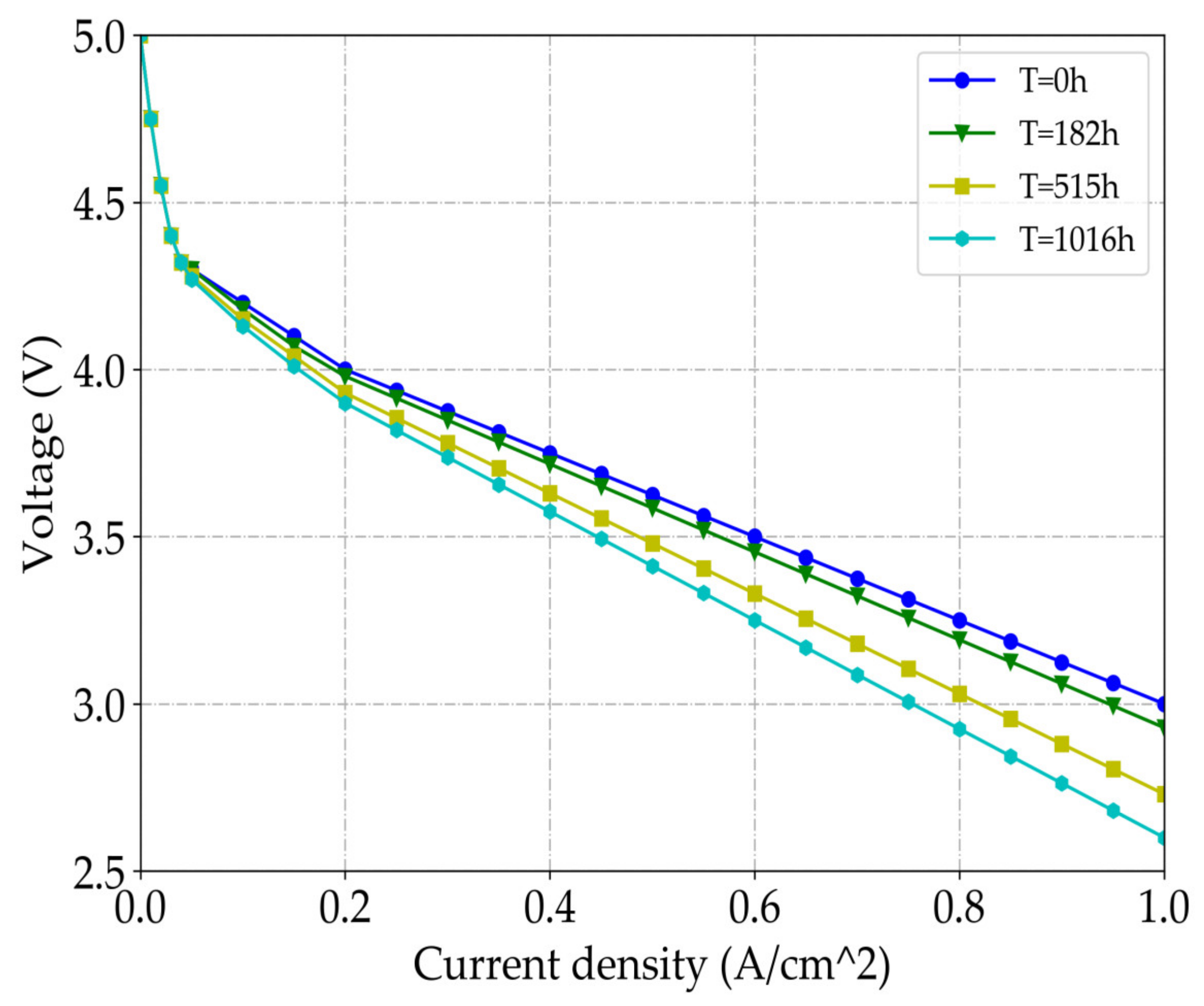
According to the evolution of the polarization curve of the PEMFC stack with the increasing operating time, the polarization curve shows a downward trend over time. As the current density increases, the voltage difference in the same current density at different times expands, as shown in Figure 2. Therefore, in order to more accurately reflect the degradation of PEMFC stack performance, it is necessary to select the stack voltage under as large an output current as possible as the health indicator. According to the statistical analysis, in all of the operating time of the fuel cell bus, the proportions of the four operating conditions were as follows: 28% for the start-stop operating condition, 43% for the 45 A operating condition, 24% for the 75 A operating condition, and 5% for the 125 A operating condition. The first three operating conditions appeared every day. To sum up, considering that both the output current and the time proportion of the selected condition should be as large as possible, the stack voltage under the 75 A operation condition was selected as the health indicator of fuel cell bus.
The daily statistical data of stack voltage mainly included the average and mode. The daily average and daily mode of the historical data of the stack voltage under 75 A operation condition were analyzed in this work. The possibility of characterizing the health status of PEMFC stack was explored through the trend of the two over time. The daily average sequence and daily mode sequence of historical data are shown in Figure 2.
The voltage of the vehicle’s on-board stack showed a slow downward trend over time under certain operation conditions. Additionally, it had significant nonlinearity and uncertainty. There were local abnormalities such as voltage recovery and random fluctuations. The above-mentioned abnormal situation may occur when an operating condition is switched or a vehicle is started and stopped. Therefore, if the daily average of stack voltage is selected as the health indicator, as shown in Figure 3a, the trend of the curve is blurred, and this value is easily affected by voltage recovery and random fluctuations. It cannot accurately characterize the degradation of stack performance. However, the daily mode of stack voltage was selected as the health indicator, as shown in Figure 3b; the curve shows a significant downward trend. It characterized the stable operating voltage of stack at the degree of degradation under the operating conditions of the day, so it could effectively avoid the influence caused by abnormal conditions and could accurately characterize the degradation of stack performance.

3. Self-Renewing RUL Prediction Model

The term self-renewing RUL prediction model refers to an RUL prediction model with self-renewing ability, one which has a strong adaptability. The self-renewing RUL prediction model proposed in this work is composed of adaptive locally weighted scatterplot smoothing (LOWESS) and Bi-LSTM RUL prediction models.

3.1. Noise Processing

The collected fuel cell operating data were a set of time series data, as shown in Figure 3, which had a certain amount of noise. Before using the data to train the model, it was necessary to perform white noise detection on the data to detect whether there were dynamic laws in the data. If the data were not white noise data, noise reduction processing could be performed on the data to improve the data quality so that the prediction results of the trained model were more accurate.
The smoothing method is often used for data noise reduction of trend analysis and prediction, using the trimming technique to weaken the influence of short-term random fluctuations on a sequence and to smooth the sequence. In this work, LOWESS was used to smooth and reconstruct the sequence, which enabled the model to effectively avoid any over-fitting caused by large data noise. In order to realize the self-renewing characteristics of the model, adaptive LOWESS was used to permit the effect of LOWESS to reach the best fit automatically.
In LOWESS, assuming that the data to be smoothed is x , y , take x as the center and intercept the data set adjacent to x , then use this data set to obtain a weighted regression line, and find the center point x , y ^ of the regression line, where y ^ is the smoothed value of x , y . If there are N sets of data, N weighted regression lines can be obtained, and the center points of the N weighted regression lines can be connected to obtain a smooth curve, which is the smoothed sequence. Before smoothing a sequence, it is necessary to select an appropriate weight function. Taking the cubic weight function in this work as an example, its weight function is defined as follows:
w i = 1 x x i d x 3 3 , x x i d x 1                             0 ,   x x i d x 1
In the Equation (1), d x is the highest power when polynomial weighted regression is used. In most application scenarios, d x is taken as 1, which is linear regression, Therefore, the weight function can be rewritten as:
w i = 1 x i 3 3 , x x i < 1 0 , x x i 1
The fitting equation can be expressed as follows:
y ^ = a x + b
The gradient a and offset b in the fitting equation can be expressed as follows:
a = w i 2 x x ¯ y y ¯ w i 2 ( x x ¯ ) 2 b = y ¯ a x ¯
where x ¯ , y ¯ are weighted averages, respectively.
The effect of using LOWESS depends on four adjustable factors, including:
  • The step size f r a c , which indicates how long the data set should be intercepted to obtain a locally weighted regression line. The f r a c is the ratio of the original data; the value range is (0,1).
  • The weight function w i , which is the above Equation (1) and can generally be a quadratic or cubic function.
  • The iteration number i t is the number of local regression operations in the selected data set.
  • The regression interval d e l t a indicates how many points are separated for a weighted regression, and the interval points can be replaced by interpolation.
Among the above four adjustable factors, the cubic weight function is used to make the method suitable for a large amount of data processing. Considering the reasonable processing time of the method, iteration number i t is 3. In order to make the smoothing effect as good as possible, the regression interval d e l t a is set to 0. The above three adjustable factors remain unchanged. This work only adjusted the step size f r a c to achieve the goal, which not only made the smoothed data sequence retain the original fluctuation to a great extent, but also weakened the influence caused by the abnormal points as much as possible.
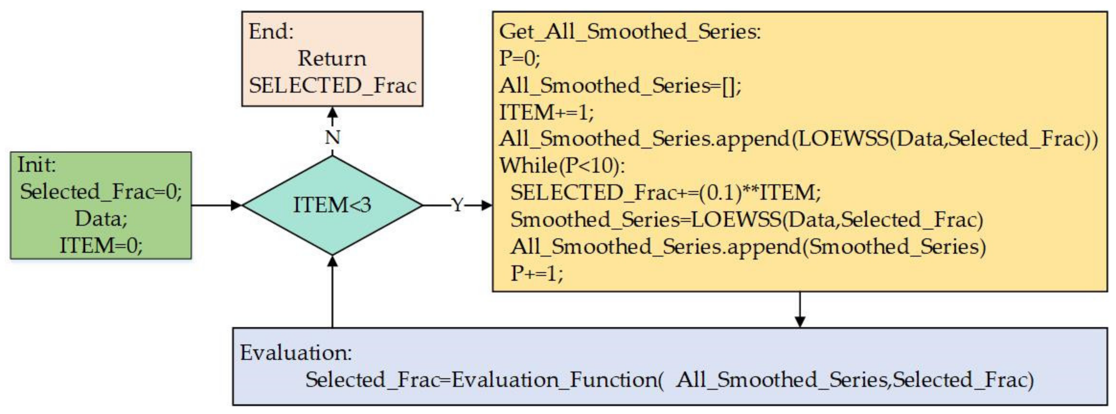
The process of adaptive LOWESS is shown in Figure 4. The adaptive LOWESS in this work could find the best f r a c , accurate to three decimal places. The realization idea is as follows:
  • Init: S e l e c t e d _ F r a c and I t e m are initialized, and then D a t a is input into the algorithm, which is the original data set.
  • The whole process is divided into three rounds—namely, 0.1 round, 0.01 round, and 0.001 round, which corresponds to items that equal 0, 1, and 2, respectively.
  • Get_All_Smoothed_Series: based on the S e l e c t e d _ F r a c found from the previous round, traverse all the LOWESS sequences of f r a c in this round; there are a total of eleven groups.
  • Evaluation: select the most suitable f r a c for this round through the evaluation function and assign it to S e l e c t e d _ F r a c .
  • If the traversal is completed, it returns S e l e c t e d _ F r a c , which is the most suitable f r a c . Otherwise, skip back to the second step to continue.
In the above process, the core point is the evaluation function. The idea of evaluation function is as follows:
Δ X f r a c _ n = X t X f r a c _ n
Δ X f r a c _ n = Δ x 1 , Δ x 2 , Δ x 3 , , Δ x j
where X t is the original sequence, X f r a c _ n is the smoothed sequence when f r a c is f r a c _ n in this round, n = 0,1,2,…,10. Δ X f r a c _ n is obtained by subtracting the smooth sequence from the original sequence.
q f r a c _ n = i = 1 Δ X f r a c _ n Δ x i 2
Considering that there may be negative numbers in Δ X f r a c _ n , the sum of squares of the sequence Δ X f r a c _ n is calculated, which is named q f r a c _ n . q f r a c _ n can better characterize the difference between the original sequence X t and the smoothed sequence X f r a c _ n .
Q = q f r a c _ 0 , q f r a c _ 1 , q f r a c _ 2 , , q f r a c _ 10
There are eleven groups of smoothed sequences X f r a c _ 0 , X f r a c _ 1 , X f r a c _ 2 , , X f r a c _ 10 in one round, and eleven corresponding q f r a c _ n can be obtained, of which a sequence Q consists.
Δ Q = D i f f Q
P f r a c = M a x Δ Q
The difference sequence Δ Q is obtained by doing a first-order difference on the sequence Q , and then the maximum value P f r a c of Δ Q is selected. P f r a c means that the LOWESS function has the largest change in the smoothed sequence due to the change of the f r a c in this round. It can be considered that the LOWESS function has the largest derivation value of the f r a c at this point. In order to keep the original fluctuation as much as possible in the smoothed sequence, the previous point of the difference segment is selected, and the most suitable f r a c is further subdivided based on the previous point.

3.2. Short-Term RUL Prediction Model

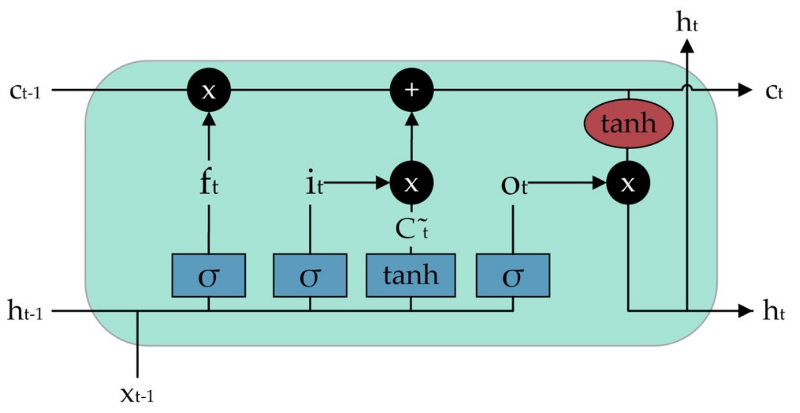
Bi-LSTM is a combination of LSTM in the forward and backward directions. The structure of LSTM is shown in Figure 5. It is composed of input word x t , cell state C t , temporary cell state C ˜ t , hidden layer state h t , forget gate f t , memory gate i t   , and input gate o t at time t . The working principle of LSTM is to convey effective information and discard useless information by forgetting and remembering information in the cell state. The hidden layer state h t is output at every time step. Forgetting, memory, and output are controlled by the forgetting gate x t memory gate i t and output gate o t , which are calculated from the current input and hidden layer state h t 1 in the previous step.
The calculation process of LSTM is as follows:
f t = σ W f h t 1 , x t + b f
First calculate the forget gate f t and select the information to be forgotten.
i t = σ W i h t 1 , x t + b i
C ˜ t = tan h W C h t 1 , x t + b C
Then calculate the memory gate i t , select the information to be memorized, and obtain the temporary cell state C ˜ t .
C t = f t * C t 1 + i t * C ˜ t
Then, according to the memory gate i t , the forget gate f t , the temporary cell state C ˜ t , and the cell state C t 1 at the previous moment, the cell state at the current moment is calculated.
o t = σ W o h t 1 , x t + b o
h t = o t * tan h C t
Finally, the output gate is calculated, and the hidden layer state at the current moment is finally obtained.
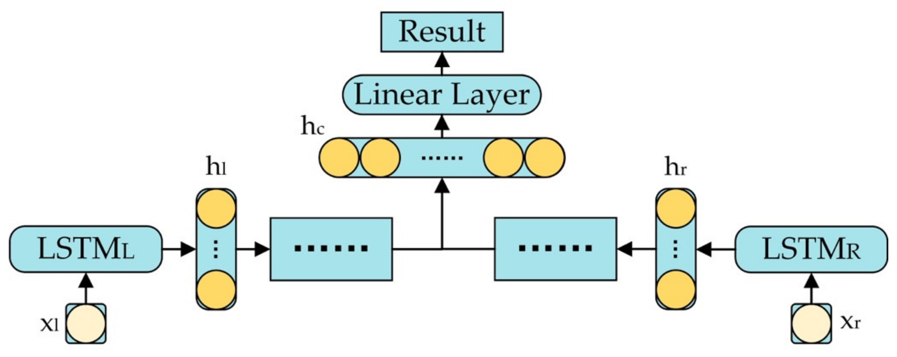
The structure of Bi-LSTM in this work is shown in Figure 6. The input vector of the model is (1,5). The output dimension of LSTM is 500, which has so sufficient a complexity that it avoids under-fitting. In order to enhance the generalization ability of the model, the value of dropout is 0.1, which can effectively avoid over-fitting. The output layer activation function is linear, the loss function of the model is MSE, and the optimizer of the model is RMSporp.

4. Online Operation Scheme on Cloud System

4.1. Cloud System

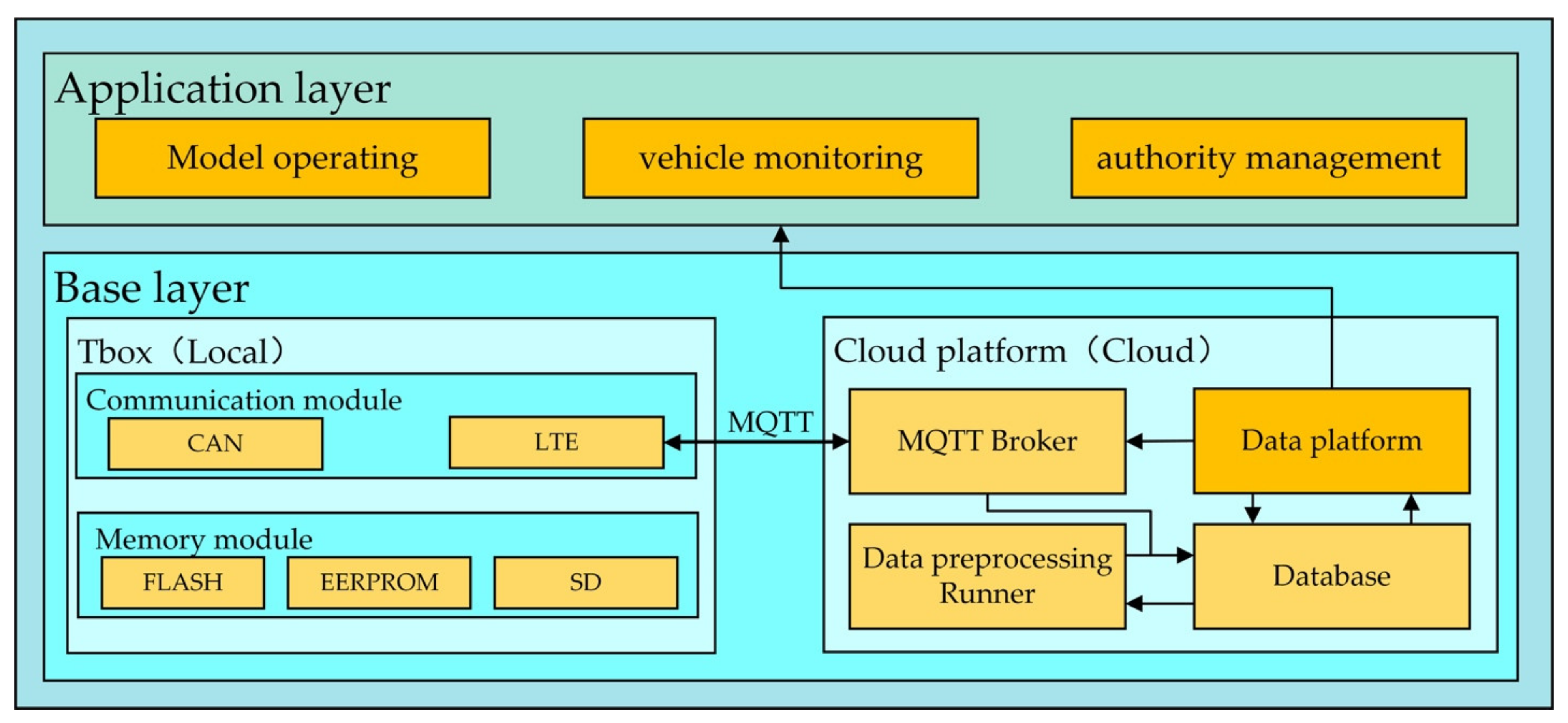
The cloud system in this work is shown in Figure 7. It consists of the base layer and the application layer.
The base layer provides the necessary basic services for the application layer. It consists of two parts: telematics box (TBOX) and cloud platform. The TBOX is placed on the fuel cell vehicle, which is at the local layer. It serves as a bridge between vehicles and cloud platforms, of which the communication protocol is message queuing telemetry transport (MQTT) protocol. Its main function is to receive the operating data from the fuel cell control unit (FCU) via CAN and upload it to the cloud platform and to receive the data from the server cloud platform and pass it to the FCU.
The cloud platform is in the cloud. It consists of an MQTT broker, data preprocessing Runner, database, and data platform. The above four modules correspond to the data transmission function, data preprocessing function, data storage function, and data application function, respectively. The MQTT broker is used for data transfer between the cloud platform and the legal TBOX. The data preprocessing Runner is used for data analysis, deduplication, and outlier detection and processing. The database is used to store data. The data platform provides staff with a visual operation platform for data application. It relies on the services provided by the first three to operate, which is between the application layer and the base layer.
The application layer relies on the data platform. It uses the data platform to call the resources of the base layer to achieve its functions. It consists of three parts: a model operation module, a vehicle monitoring module, and an authority management module. The first two modules are used to manage fuel cell vehicles through the cloud system, and the latter is used to manage the personnel who use the cloud system. The self-renewing RUL prediction model of this work was deployed in the model operation module.
The above is the architecture of the fuel cell vehicle cloud system in this work. The online operations of the self-renewing RUL prediction model are realized through the cloud system.

4.2. Online Operation Scheme

The process of the self-renewing short-term RUL prediction scheme based on the cloud system is shown in Figure 8. The specific process is as follows:
  • The data platform has a RUL prediction task detector, which checks daily whether the model needs to be updated. Its judgment condition of trigger is whether the number of days from the last execution time of a task exceeds its update days (the number of update days is set to 5 days). If so, model training is triggered.
  • Before the data denoising process, it is necessary to analyze whether the sequence is a white noise sequence. In the second step, historical data are taken out to perform white noise detection on them. Acorr-Ljung-Box was used to verify whether the data in this work were white noise. The l a g s is set to 1. S t a t and P is calculated. The Stat is the Ljung–Box test statistic. The P value is the evidence against a null hypothesis. The smaller the P value, the stronger is the evidence for rejecting the null hypothesis. If P is less than 0.05—that is, the data are not white noise data—skip to the third step. Otherwise, the cloud platform alarm is triggered for human intervention.
  • Using adaptive LOWESS to smooth and denoise the data, the smoothed data are normalized and regularized to improve model training.
  • The Glorot normal distribution is used to initialize the input weights, and the uniform random distribution is used to initialize the hidden layer threshold, which effectively avoid under-fitting to a certain extent. Subsequently, the data are input into the Bi-LSTM model for training.
  • The health indicator value of vehicle stack in the next five days is predicted through the trained model, followed by storage of the results in the cloud platform database.

5. Simulation Experimental Environment

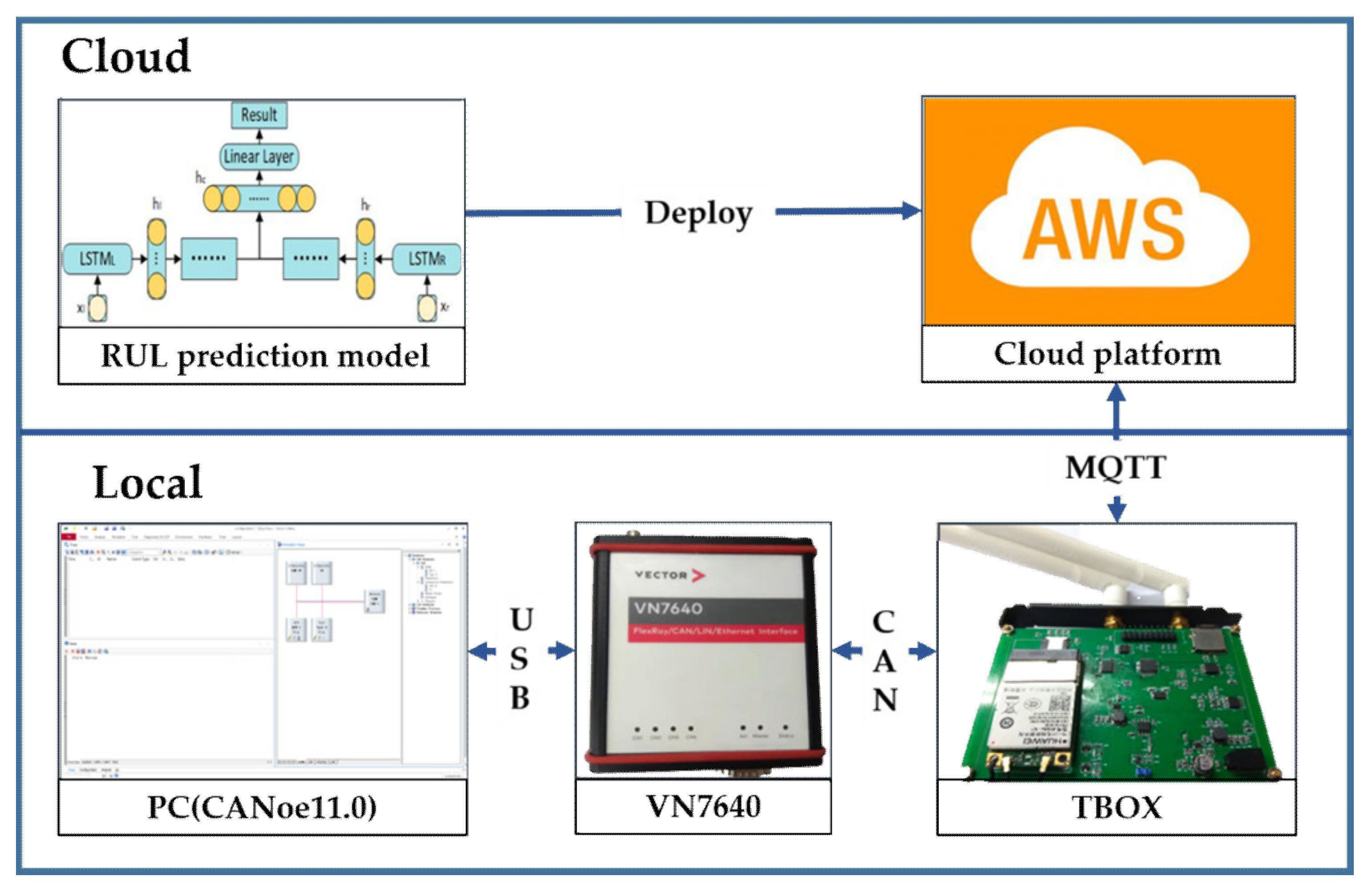
A simulation experimental environment was built to verify the online operation scheme. The details are shown in Figure 9 and items of the simulated experimental environment are shown in Table 3. The fuel cell bus was simulated by VECTOR VN7640 hardware interface card and CANoe11.0 software. VN7640 was connected with TBOX through CAN and communicated with a PC running VN7640 through USB. The TBOX was connected with the cloud system through MQTT. The data studied in this work were historical data of the fuel cell bus. In the experiment, historical data of fuel cell bus were read from storage files by CANoe11.0 and sent to TBOX by VN7540, then TBOX sent the received data to the cloud system, on which the self-renewing RUL prediction model was deployed. After the data were stored in the cloud system, the process was executed as described in Section 4.2 to realize short-term RUL prediction.

6. Result and Discussion

6.1. Validation of Adaptive LOWESS and Bi-LSTM RUL Prediction Model

In this experiment, the historical data from 1 to 122 days were used as the training set to predict the stack voltage of a fuel cell bus under 75 A operating condition in the subsequent five days (123 to 127 days).
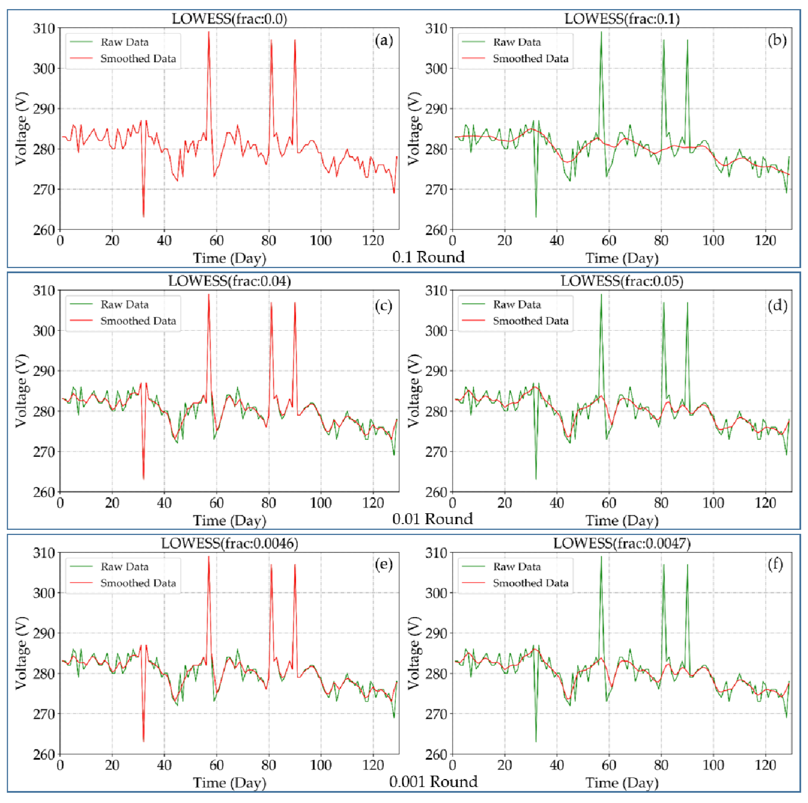
Firstly, the data of the following model training were all processed by adaptive LOWESS and normalized. Figure 10 shows the operation steps and effects of adaptive LOWESS. In the first round, the appropriate f r a c segment in the 0.1 round was screened, and the appropriate f r a c was found between 0 and 0.1. In the second round, the appropriate f r a c segment in the 0.01 round was screened, and the appropriate f r a c was found between 0.04 and 0.05. In the third round, the appropriate f r a c in the 0.001 round was screened. After three rounds of screening, the most suitable f r a c was finally obtained as 0.047. As shown in Figure 10, the processed voltage curve is relatively smooth, which is effectively denoised. But it retains the change trend of the original data, which is helpful for subsequent RUL prediction model training.
Secondly, the epochs of training were set to 50 times and the b a t c h _ s i z e was set to 32. Subsequently, the smoothed sequence was put into the model to train. The predicted results of the model after training are shown in Figure 11. The size and trend of the predicted voltage curve are basically consistent with the actual voltage curve, which shows that the fitting effect is worked well. The model predicted the stack voltage of the fuel cell vehicle under 75 A operating condition over the subsequent five days, which was 275.90 V, 275.70 V, 275.35 V, 274.78 V, and 275.01 V. Meanwhile, the actual stack voltage was 275.64 V, 275.39 V, 274.88 V, 274.12 V, and 274.83 V. It is worth noting that, as marked by the black circle in Figure 11, the model could effectively predict that the trend of stack voltage turned from a downward trend to an increasing trend on the fifth day. In the actual data, the stack voltage also showed an upward trend in the next two days (128 to 129 days), 276.16 V and 277.48 V, respectively.
In this work, Bi-LSTM, LSTM, and 1D-CNN were compared to prove that Bi-LSTM is superior to other models. Root mean square error (RMSE), mean absolute error (MAE), and mean absolute percentage error (MAPE) were selected to verify the accuracy of the model in this work. The results are shown in Table 4. The RMSE, MAE, and MAPE of Bi-LSTM were all smaller than the others. Thus, Bi-LSTM had better fitting accuracy and smaller relative error, which suggests that it is more suitable for short-term RUL prediction of a PEMFC stack.

6.2. Verification of Online Operation Scheme of Self-Renewing Short-Term RUL Prediction Model

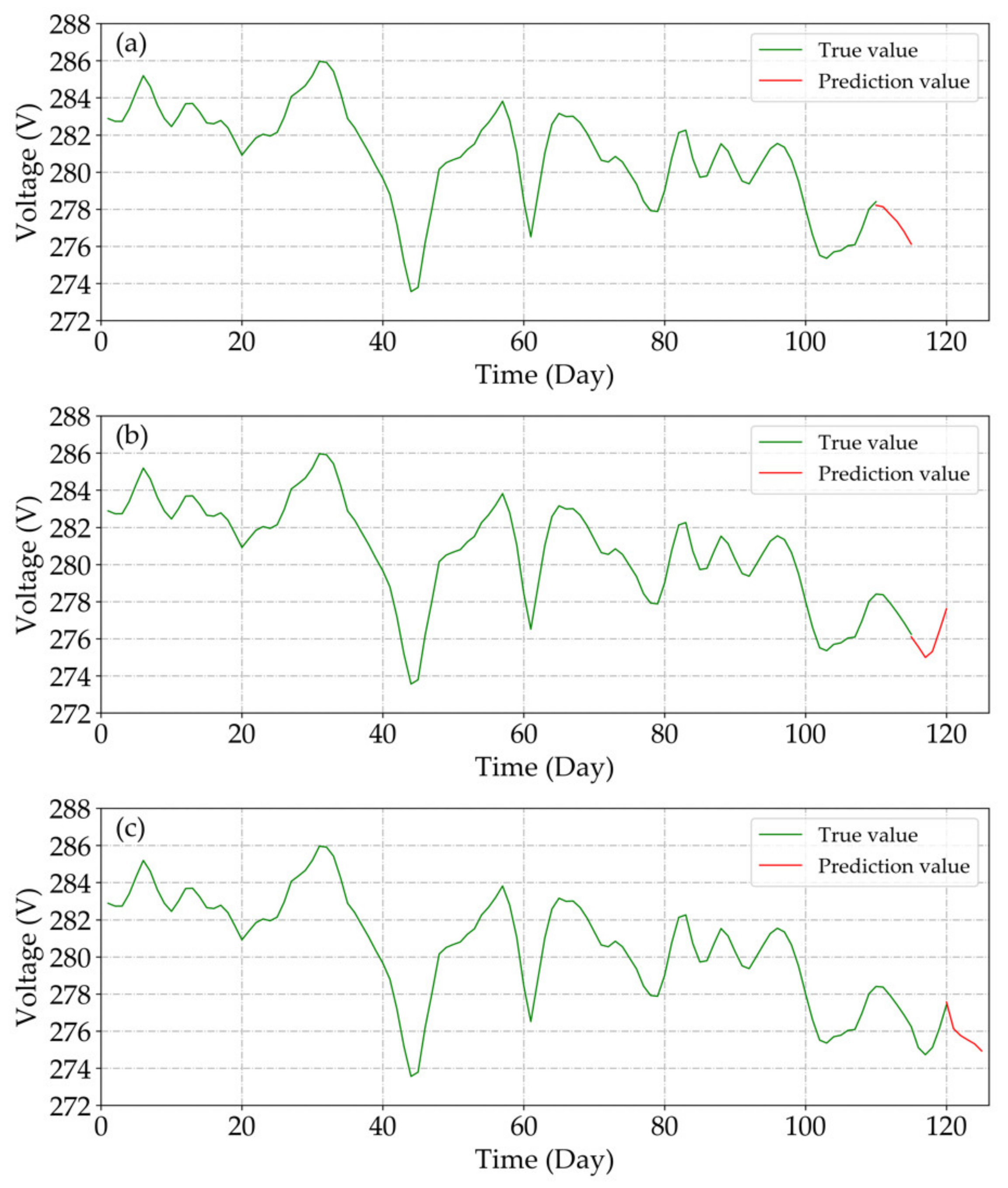
This experiment was divided into three rounds. The initial day of the experiment started from the 110th day of the fuel cell bus. The simulation days of each round were 5 days—the prediction days of the RUL prediction model. In the test, when data of each round had been uploaded to the server, the model was triggered to renew itself.
Firstly, the data were taken out from the database of the cloud system and white noise detection was performed on the data. The results of white noise detection are shown in Table 5. P of the three sets of sequences in the table are all less than 0.05; that is, the three sets of sequences are not white noise sequences, which have dynamic laws that can be used. The platform alarm was not triggered, and the next step could be executed. It was verified that selecting the daily mode of stack voltage under 75 A operation condition as a health indicator can effectively reflect the degradation of the fuel cell stack.
Furthermore, adaptive LOWESS was performed on the sequence. Through the adaptive LOWESS, the best f r a c of the 1–110-day data sequence was obtained, which was 0.055; the best f r a c of the 1–115-day data sequence was obtained as 0.053, and 0.050 was the best f r a c of the 1–120-day data sequence. The three sets of curves processed by the adaptive LOWESS are shown in Figure 12. The three sets of smoothed sequences not only effectively retained the trend of the original sequence, but also effectively suppressed the noise. This verifies that the adaptive LOWESS has excellent effectiveness and robustness.
Finally, the RUL prediction model was trained with the smoothed sequence, and the corresponding health indicator values of the fuel cell stack in the next five days were obtained, which are shown in Table 6. The MAE values of the prediction results of the three rounds were 0.162, 0.298, and 0.102, respectively. The RMSE values of the three rounds were 0.172, 0.327, and 0.109, respectively. The values are so small that they demonstrate the good accuracy of the model from different aspects. The MAPE values of the three rounds were 0.058%, 0.108%, and 0.037%. These values are extremely close to zero, which proves that the quality of the model is quite good. Compared with other rounds, the values of the second round were larger. Through analysis, it was found that there is a positive inflection point of voltage slope in the second round, and it increases or decreases monotonically in other rounds. Figure 13 presents curves of prediction results of the self-renewing RUL prediction model. It can be seen clearly that although there is a slight error in prediction results, the trend and value of prediction sequence in each round can be quite accurate.
To sum up, the strong adaptability and prediction accuracy of the self-renewing RUL prediction model and the effectiveness of online operation function were verified.

7. Conclusions

The durability of automotive PEMFCs is one of the main factors restricting their commercial application. One of the effective ways to improve the durability of automotive PEMFCs is to develop an accurate and strong practical RUL prediction model and an online operation method of RUL prediction model. In this paper, based on the historical data of a fuel cell bus, a self-renewing RUL prediction model was established, and an online operation scheme that could be relayed on the system was proposed, both of which realize short-term online RUL prediction for automotive PEMFC stacks. The main conclusions are as follows:
  • The mode of daily stack voltage of 75 A operation condition used as the health index of the fuel cell bus stack avoided the influence of voltage recovery and random fluctuation. White noise detection can be used to verify that the parameter can better characterize the stack health state.
  • The adaptive LOWESS and Bi-LSTM RUL prediction model was established. Adaptive LOWESS is used for adaptive denoising and preliminary feature extraction of stack voltage data, which not only enables the smoothed data series to retain the original fluctuation as much as possible, but also weakens the influence of abnormal points as much as possible. Subsequently, a Bi-LSTM model can be trained with the denoised sequence to realize short-term RUL prediction, which proved to be quite accurate and to have strong adaptability.
  • Relying on TBOX and a cloud platform to realize real-time data updating, an online operation scheme of short-term RUL prediction scheme model is proposed, which realizes the short-term online prediction of RUL. The scheme was proved to be effective, which gives the model a strong powerful practicability.
In summary, this work has improved the technology route of PEMFC RUL prediction in vehicles and has good prospects for application in the prognostic and health management of PEMFCs, which is helpful for improving the durability of automotive PEMFCs.

Author Contributions

Conceptualization, T.M. and J.X.; methodology, J.X.; software, J.X.; validation, J.X., N.Y., and R.L.; formal analysis, T.M.; investigation, J.X.; resources, T.M.; data curation, J.X.; writing—original draft preparation, T.M. and J.X.; writing—review and editing, Y.Y., N.Y., and R.L.; visualization, J.X.; supervision, J.X., N.Y., and Y.Y.; project administration, T.M. All authors have read and agreed to the published version of the manuscript.

Funding

This research received no external funding.

Acknowledgments

This work was funded by the Key-Area Research and Development Program of Guangdong Province (No. 2019B090909002).

Conflicts of Interest

The authors declare no conflict of interest.

References

  1. Anderson, R.; Zhang, L.; Ding, Y.; Blanco, M.; Bi, X.; Wilkinson, D.P. A critical review of two-phase flow in gas flow channels of proton exchange membrane fuel cells. J. Power Sources 2010, 195, 4531–4553. [Google Scholar] [CrossRef]
  2. Hu, G.; Fan, J.; Chen, S.; Liu, Y.; Cen, K. Three-dimensional numerical analysis of proton exchange membrane fuel cells (PEMFCs) with conventional and interdigitated flow fields. J. Power Sources 2004, 136, 1–9. [Google Scholar] [CrossRef]
  3. Wu, J.; Yuan, X.Z.; Martin, J.J.; Wang, H.; Zhang, J.; Shen, J.; Wu, S.; Merida, W. A review of PEM fuel cell durability: Degradation mechanisms and mitigation strategies. J. Power Sources 2008, 184, 104–119. [Google Scholar] [CrossRef]
  4. Liu, H.; Chen, J.; Hissel, D.; Lu, J.; Hou, M.; Shao, Z. Prognostics methods and degradation indexes of proton ex-change membrane fuel cells: A review. Renew. Sustain. Energy Rev. 2020, 123, 109721. [Google Scholar] [CrossRef]
  5. Jouin, M.; Gouriveau, R.; Hissel, D.; Péra, M.-C.; Zerhouni, N. Degradations analysis and aging modeling for health assessment and prognostics of PEMFC. Reliab. Eng. Syst. Saf. 2016, 148, 78–95. [Google Scholar] [CrossRef]
  6. Zhang, X.; Pisu, P. Prognostic-oriented Fuel Cell Catalyst Aging Modeling and Its Application to Health-Monitoring and Prognostics of a PEM Fuel Cell. Int. J. Progn. Health Manag. 2014, 5, 1–16. [Google Scholar] [CrossRef]
  7. Yin, S.; Xie, X.; Lam, J.; Cheung, K.C.; Gao, H. An Improved Incremental Learning Approach for KPI Prognosis of Dynamic Fuel Cell System. IEEE Trans. Cybern. 2015, 46, 3135–3144. [Google Scholar] [CrossRef]
  8. Qiao, L.Q.; Xun, L.J. State of health estimation combining robust deep feature learning with support vector regression. In Proceedings of the 2015 34th Chinese Control Conference (CCC), Hangzhou, China, 28–30 July 2015; pp. 6207–6212. [Google Scholar]
  9. Wu, Y.; Breaz, E.; Gao, F.; Paire, D.; Miraoui, A. Nonlinear Performance Degradation Prediction of Proton Exchange Membrane Fuel Cells Using Relevance Vector Machine. IEEE Trans. Energy Convers. 2016, 31, 1570–1582. [Google Scholar] [CrossRef]
  10. Bressel, M.; Hilairet, M.; Hissel, D.; Bouamama, B.O. Remaining useful life prediction and uncertainty quantifica-tion of proton exchange membrane fuel cell under variable load. IEEE Trans. Ind. Electron. 2016, 63, 2569–2577. [Google Scholar] [CrossRef]
  11. Jouin, M.; Gouriveau, R.; Hissel, D.; Péra, M.-C.; Zerhouni, N. Prognostics of PEM fuel cell in a particle filtering framework. Int. J. Hydrogen Energy 2014, 39, 481–494. [Google Scholar] [CrossRef] [Green Version]
  12. Ibrahim, M.; Steiner, N.Y.; Jemei, S.; Hissel, D. Wavelet-based approach for online fuel cell remaining useful life-time prediction. IEEE Trans. Ind. Electron. 2016, 63, 5057–5068. [Google Scholar]
  13. Liu, J.; Saxena, A.; Goebel, K.; Saha, B.; Wang, W. An Adaptive Recurrent Neural Network for Remaining Useful Life Prediction of Lithium-Ion Batteries. In Proceedings of the Annual Conference of the Prognostics and Health Management Society, Portland, OR, USA, 10–16 October 2010. [Google Scholar]
  14. Heimes, F.O. Recurrent neural networks for remaining useful life estimation. In Proceedings of the 2008 International Conference on Prognostics and Health Management, Denver, CO, USA, 6–9 October 2008; pp. 1–6. [Google Scholar]
  15. Morando, S.; Jemei, S.; Hissel, D.; Gouriveau, R.; Zerhouni, N. Proton exchange membrane fuel cell ageing fore-casting algorithm based on Echo State Network. Int. J. Hydrogen Energy 2017, 42, 1472–1480. [Google Scholar] [CrossRef]
  16. Ma, R.; Breaz, E.; Liu, C.; Bai, H.; Briois, P.; Gao, F. Data-driven Prognostics for PEM Fuel Cell Degradation by Long Short-term Memory Network. In Proceedings of the 2018 IEEE Transportation Electrification Conference and Expo (ITEC), Long Beach, CA, USA, 13–15 June 2018; pp. 102–107. [Google Scholar]
  17. Liu, J.; Li, Q.; Chen, W.; Yan, Y.; Qiu, Y.; Cao, T. Remaining useful life prediction of PEMFC based on long short-term memory recurrent neural networks. Int. J. Hydrogen Energy 2019, 44, 5470–5480. [Google Scholar] [CrossRef]
  18. Ma, J.; Liu, X.; Zou, X.; Yue, M.; Shang, P.; Kang, L.; Jemei, S.; Lu, C.; Ding, Y.; Zerhouni, N.; et al. Degradation prognosis for proton exchange membrane fuel cell based on hybrid transfer learning and intercell differences. ISA Trans. 2020. [Google Scholar] [CrossRef]
  19. Ma, R.; Yang, T.; Breaz, E.; Li, Z.; Briois, P.; Gao, F. Data-driven proton exchange membrane fuel cell degradation predication through deep learning method. Appl. Energy 2018, 231, 102–115. [Google Scholar] [CrossRef]
  20. Liu, J.; Li, Q.; Yang, H.; Han, Y.; Jiang, S.; Chen, W. Sequence fault diagnosis for PEMFC water management sub-system using deep learning with t-SNE. IEEE Access 2019, 7, 92009–92019. [Google Scholar] [CrossRef]
  21. Xue, X.; Hu, Y.; Qi, S. Remaining useful life estimation for proton exchange membrane fuel cell based on extreme learning machine. In Proceedings of the 2016 31st Youth Academic Annual Conference of Chinese Association of Automation (YAC), Wuhan, China, 11–13 November 2016; pp. 43–47. [Google Scholar]
  22. Javed, K.; Gouriveau, R.; Zerhouni, N.; Hissel, D. Prognostics of Proton Exchange Membrane Fuel Cells stack using an ensemble of constraints based connectionist networks. J. Power Sources 2016, 324, 745–757. [Google Scholar] [CrossRef]
  23. Jacome, A.; Hissel, D.; Heiries, V.; Gerard, M.; Rosini, S. A Review of Model-Based Prognostic for Proton Exchange Membrane Fuel Cell under Automotive Load Cycling. In Proceedings of the 2019 IEEE Vehicle Power and Propulsion Conference (VPPC), Hanoi, Vietnam, 14–17 October 2019; pp. 1–5. [Google Scholar]
  24. Hua, Z.; Zheng, Z.; Péra, M.C.; Gao, F. Remaining useful life prediction of PEMFC systems based on the mul-ti-input echo state network. Appl. Energy 2020, 265, 114791. [Google Scholar] [CrossRef]
  25. Sutharssan, T.; Montalvao, D.; Chen, Y.K.; Wang, W.-C.; Pisac, C.; Elemara, H. A review on prognostics and health monitoring of proton exchange membrane fuel cell. Renew. Sustain. Energy Rev. 2017, 75, 440–450. [Google Scholar] [CrossRef] [Green Version]
  26. Jouin, M.; Gouriveau, R.; Hissel, D.; Péra, M.C.; Zerhouni, N. Joint particle filters prognostics for PEMFC power prediction at constant current solicitation. IEEE Trans. Reliab. 2016, 65, 336–349. [Google Scholar] [CrossRef]
  27. Kim, T.; Oh, H.; Kim, H.; Youn, B.D. An Online-Applicable Model for Predicting Health Degradation of PEM Fuel Cells with Root Cause Analysis. IEEE Trans. Ind. Electron. 2016, 63, 7094–7103. [Google Scholar] [CrossRef]
  28. FCLAB Federation, FR CNRS 3539, France. FCLAB. 2014. IEEE PHM 2014 Data Challenge. Available online: http://eng.fclab.fr/ieee-phm-2014-data-challenge (accessed on 1 May 2014).
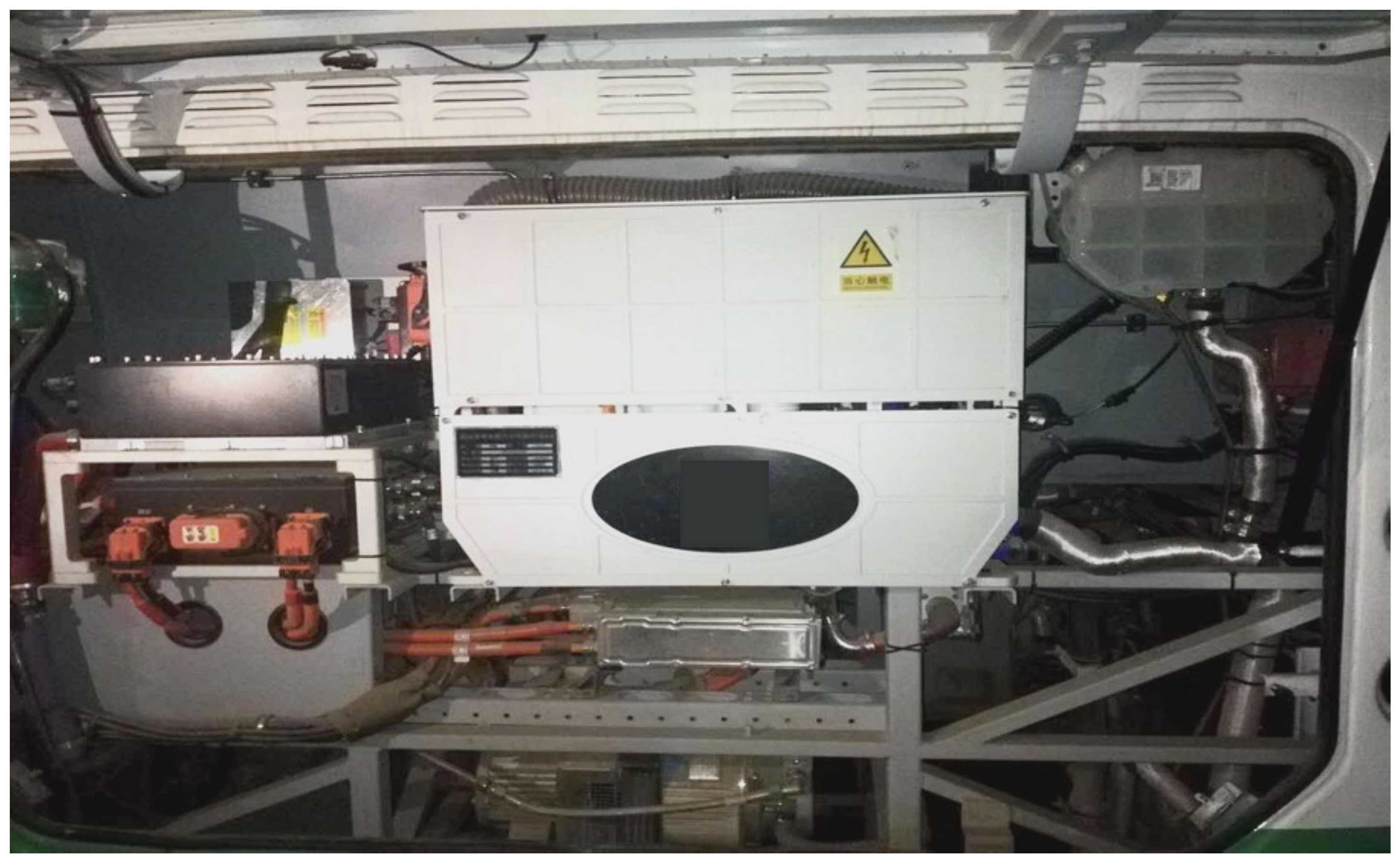
Figure 1. System of experimental fuel cell bus.
Energies 14 02806 g001
Figure 2. Polarization curves of the fuel cell stack FC2 at different time periods from IEEE PHM 2014 data challenge [28].
Energies 14 02806 g002
Figure 3. (a) Daily average sequence of stack voltages under 75 A operating condition; (b) daily mode sequence of stack voltages under 75 A operating condition.
Energies 14 02806 g003
Figure 4. Flow chart of adaptive LOWESS (Python pseudocode).
Energies 14 02806 g004
Figure 5. The structure of LSTM.
Energies 14 02806 g005
Figure 6. The structure of Bi-LSTM.
Energies 14 02806 g006
Figure 7. Cloud system architecture.
Energies 14 02806 g007
Figure 8. Flow chart of online operation of self-renewing model.
Energies 14 02806 g008
Figure 9. Display of simulation experimental environment.
Energies 14 02806 g009
Figure 10. Effects of adaptive LOWESS in every round: (a,b) the effects in the 0.1 round; (c,d) the effect in the 0.01 round; (e,f) the effects in the 0.001 round.
Energies 14 02806 g010
Figure 11. Prediction result of adaptive LOWESS and Bi-LSTM RUL prediction model.
Energies 14 02806 g011
Figure 12. Effects of adaptive LOWESS: (a) the effect in the first round; (b) the effect in the second round; (c) the effect in the third round.
Energies 14 02806 g012
Figure 13. Curves of prediction results of self-renewing RUL prediction model: (a) the prediction results in the first round; (b) the prediction results in the second round; (c) the prediction results in the third round.
Energies 14 02806 g013
Table 1. The specification of stack in fuel cell bus.
NameValue
Brand of fuel cell stackPOWERCELL S2 Series
Number of cells in fuel cell stack432 pieces
Rated Power40 kW
Max Efficiency55%
Stack mass31 kg
Table 2. Necessary system parameters of operating conditions.
ParameterValue
Operating Condition45 A75 A125 A
System Air Inlet Flow Rate900 Slpm1300 Slpm2100 Slpm
Stack Hydrogen Inlet Pressure13 Kpa13 Kpa14.5 Kpa
Stack Hydrogen Outlet Pressure12.8 Kpa12.7 Kpa14.1 Kpa
Stack Inlet Temperature70 °C70 °C70 °C
Stack Outlet Temperature71 °C72 °C74 °C
Table 3. Items of simulation experimental environment.
ItemsManufacturersFunction
CANoe11.0 softwareVECTORRead data from storage files
VN7640 hardware interfaceVECTORSend data to TBOX
TBOXSelf-developedSend data to Cloud System
Cloud SystemAmazon1. Receive and store data from the local
2. Execute the online operation schema
Table 4. Comparison of the prediction results of three models.
ModelRMSEMAEMAPE
Bi-LSTM0.4130.3760.136%
LSTM0.6510.5910.215%
1D-CNN0.9720.9250.336%
Table 5. White noise detection results of three sets of experimental sequence.
SequenceStatP
1–110 days sequence4.370319130.03657014
1–115 days sequence5.697568580.01698843
1–120 days sequence0.00392990.0039299
Table 6. The prediction results of three sets of experimental sequence.
RoundPrediction DayPrediction ValueTrue ValueMAERMSEMAPE
1111278.13278.370.1620.1720.058%
112277.72277.92
113277.33277.41
114276.68276.85
115276.12276.24
2116275.67275.110.2980.3270.108%
117274.99274.73
118275.31275.11
119276.43276.15
120277.61277.42
3121276.13275.960.1020.1090.037%
122275.76275.66
123275.53275.64
124275.31275.39
125274.93274.88
Publisher’s Note: MDPI stays neutral with regard to jurisdictional claims in published maps and institutional affiliations.