Analysis of Thermodynamic Parameter Variability in a Chamber of a Furnace for Thermo-Chemical Treatment

Abstract

This paper presents results of research on unevenness of cylinder heating in a furnace for thermo-chemical treatment. Experimental research was conducted with respect to nitriding. Various heating speeds and settings of the fan operation in the furnace were considered. Boundary conditions were calculated in the form of temperature and the heat transfer coefficient (HTC) on the cylinder boundary in four planes along the cylinder length. Calculations were performed with the use of the inverse problem for non-linear and unsteady heat conduction equations. Boundary conditions from individual planes were compared with the mean value of them all. The variability of the calculated boundary conditions (temperature and HTC) along the cylinder length was investigated based on values of the absolute and relative differences for temperature and HTC. Estimates: mean value, mean value from the absolute value and the maximum values for the absolute and the relative differences of temperature and HTC were also calculated. Estimates were the measurements of the unevenness of cylinder heating in a furnace for thermo-chemical treatment. Based on the results of our research, it was found that an increase of the fan rotational speed from 50% to 100%, with the same heating speed, resulted in a significant leveling of temperature in the analyzed planes. The difference in temperature along the cylinder length was reduced from 6.8 °C to 3.3 °C. The increase of the heating speed from 5 °C/min to 10 °C/min resulted in an increase of the unevenness of the cylinder heating. Values of the absolute differences of temperature in the analyzed planes with reference to the mean temperature changed from an interval from −2.7 °C to 2.3 °C to a range from −4 °C to 5 °C. In processes with a heating speed greater than 5 °C/min, more intensive heating in the end part of the cylinder (close to the cylinder) was achieved than it was in other planes. It was proven by temperature values, which were higher, even, by 5.4 °C, and by HTC values, higher by 11.4 W/m²K, when compared with mean values. Obtained results can form the basis for nitriding process optimization.

1. Introduction

Many elements of machines are subject to thermo-chemical treatments such as nitriding or carburizing. Such treatments are used to create metal layers with desired properties. Layer creation is correlated with the value of temperature on the element’s boundary, which is impossible to measure with good accuracy during the process. Particularly complicated are treatment processes of massive elements with complex geometry. Elements being treated should not be damaged due to too-high thermal stresses. For economic reasons, the heating of charges as quickly as possible and a charge soaking as short as possible are most desired. Thorough knowledge of temperature on the boundary of the element under treatment enables choosing the maximum heating speed for which thermal stresses are not exceeded. Temperature on the boundary of the element being treated is the information enabling application of gases such as ammonia or nitrogen at the most proper stages of the process. Analyses of heat treatment processes are performed based on selected optimization criteria such as time, costs or the quality of the formed surface layer. Determination of the boundary condition (temperature, heat flux or the heat transfer coefficient) is helpful for optimizing processes of heat or thermo-chemical treatment. Determination of the boundary condition is possible based on temperature measurement inside the element and by then solving the inverse problem for the heat equation [1,2,3,4]. In the next step, the distribution of temperature in the element is determined based on the boundary condition by solving the direct problem. Inverse problems are ill-conditioned numerically [5]. Many papers concerning algorithms for solving inverse problems [6,7,8,9,10,11,12,13] and presenting analyses of their stability [14,15,16] have been written to date. Inverse problems were used to analyze laser treatment of metal elements [17,18].

Analysis of cylinder heating in a furnace for thermo-chemical treatment was presented in a paper [19]. Boundary conditions were obtained from the solution of a non-stationary, non-linear inverse problem for the heat equation. The impact of the time step, the regularization parameter, on solution stability, was investigated.

The inverse heat conduction problem (IHCP) was also applied in a newly designed thermometer [20]. This thermometer was used to determine fluid temperatures and heat transfer coefficients on the internal surfaces of boilers’ elements. Investigated elements of boilers were subjected to high thermal stresses during plant start-up and shutdown. The newly designed thermometer enabled on-line control of thermodynamic parameters and arising thermal stresses. Such a thermometer was also applied to a system of temperature settings in a hot liquid tank heated with electric energy [21].

Thermo-physical properties of a material of substance such as thermal conductivity or specific heat are crucial for thermodynamic calculations. The variability of these properties significantly affects the analysis of heat flow [19,22,23] including obtained boundary conditions and, particularly, HTC. Knowledge of values of temperature and of the heat transfer coefficient on the boundary is crucial when we consider thermal machine and device operation. Many methods of determining the HTC are described in the scientific literature. Iterative methods are among the widely used methods [24]. A paper [25] presented research on determining the HTC in a cylindrical combustion chamber fed with hard coal and biomass. The involvement of convection and radiation in the heat flow of a heating device was analyzed. Methods for the calculation of HTC in mini channels with the use of the Beck method and Trefftz functions are presented in a paper [26]. Analyzed solutions to the inverse problem gave comparable values to the sought boundary condition. The determination of boiling HTC in mini channels by solving IHCP was also discussed in papers [27,28]. A paper [29] discusses determination of the HTC in a T-shaped cavity. It includes a comparison of the value of the HTC obtained from the solution of the inverse problem and of a 2D analytic thermal network.

The research problem considered in this paper is related to the determination of temperature and the HTC on the cylinder boundary. Experimental tests were conducted with respect to nitriding processes. Temperature on the cylinder boundary was determined by solving the inverse problem for the heat equation. This paper is a continuation of research work presented in paper [19]. Paper [24] includes a description of the algorithm for solving the inverse problem and investigation of its numerical stability. That algorithm was applied to the calculation of boundary conditions in one measuring plane in the cylinder. This paper presents results of temperature and HTC calculations, performed in four planes along the cylinder length. Obtained values were compared to mean [average] values. Research enabled us to analyze the change in boundary conditions along the length of the cylinder being heated in the furnace for thermo-chemical treatment, which had not been included in the paper [24]. Quantitative knowledge on temperature and HTC differences occurring on the cylinder boundary is the basis for the analysis of the unevenness of load heating in furnaces for thermo-chemical treatment. The difference between temperatures in the cylinder axis and on the cylinder boundary was also considered. These data constitute a basis for optimizing the processes of thermo-chemical treatment.

2. The Scope of Experimental Research

Experimental research was performed in a chamber furnace with a cylindrical shape and horizontal loading (Figure 1). This furnace operates in cycles. A fan forces the movement of the atmosphere in the working chamber of the furnace. It sucks in gas from the area of the working chamber and next pumps it through the annular channel, where gas flowing toward the furnace door is heated. Three heat sources are placed behind the wall of the working chamber, along the annular channel. In the vicinity of the furnace door, the geometry of the cylindrical partition causes a change in the main direction of gas flow by 180°. A diagram of the furnace construction and of the cylinder placed inside the furnace with marked measuring planes is shown in Figure 1. The location of measuring planes A1–A4 is described in

Table 1. Location of planes A1–A4 along the cylinder length.

Plane	Distance from the Top of the Cylinder [mm]
A1	186
A2	252
A3	318
A4	384

.

Experimental tests included the measurement of the gas temperature in the furnace and of the temperature inside the cylinder of diameter D = 100 mm, made of steel. Thermocouples were located on the radius r₁* = 48 mm (at the distance g = 2 mm from the cylinder boundary in planes A1, A2 and A4). In plane A3, thermocouples were located on radii r₁* = 44 mm, r₂* = 46 mm and r₃* = 48 mm. The thermocouple installation error was Δr = ±0.2 mm. Temperature was measured with the use of K-type thermocouples, nickel–chromium–nickel. The course of the error assumed for the experiment in temperature measurement ET was revealed by points determined during the calibration process and connected with straight lines (Figure 2).

The cylinder was heated in the nitrogen atmosphere from the ambient temperature to temperature T_max = 550 °C. Heating speeds set in the furnace were equal to 5, 6, 8 and 10 °C/min. The fan rotational speed provided 50 and 100% of the maximum speed equal to 2800 rev/min (

Table 2. Parameters of heating processes.

Process	Heating Speed [°C/min]	Fan Settings [%]
p1	5	50
p2	5	100
p3	6	50
p4	8	50
p5	10	50

).

Based on the analysis of errors in temperature and HTC on the cylinder boundary, we determined times at which admissible results of errors were obtained (

Table 3. Minimum and maximum times for which admissible values of temperature and HTC error on the cylinder boundary were obtained for processes p1–p5.

	p1	p2	p3	p4	p5
tmin [s]	930	390	1020	750	330
tmax [s]	12,600	9870	11,400	9870	9240

). A detailed analysis of errors for plane A3 was presented in paper [19].

3. Calculation Model

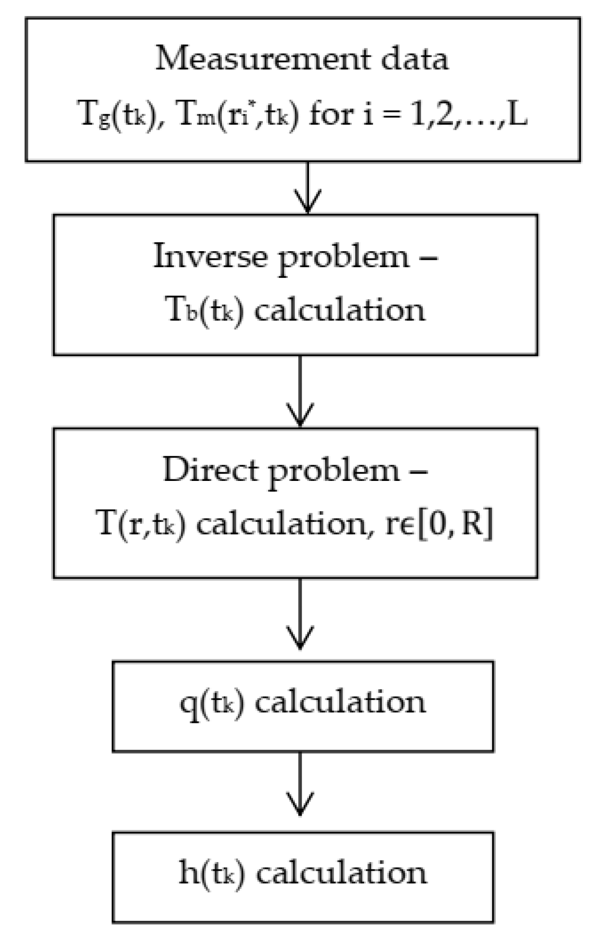
In processes of thermo-chemical treatment such as nitriding, it is impossible to determine the temperature on the boundary of the element under treatment with good accuracy. This temperature can be found by measuring the temperature inside the solid body and solving the inverse problem (Figure 3).

To determine temperature on the cylinder boundary T_b(t_k), a non-stationary heat equation of the following form was solved:

$$\mathsf{\rho }\left(\mathrm{T}\right)\mathrm{c}\left(\mathrm{T}\right)\frac{\partial \mathrm{T}}{\partial \mathrm{t}}=\mathrm{div}\left(\mathsf{\lambda }\left(\mathrm{T}\right)\nabla \mathrm{T}\right)$$

(1)

A one-dimensional, non-linear problem of heat conduction in the cylinder was analyzed. Nonlinearity resulted from the dependence of density ρ(T), specific heat c(T) and the thermal conductivity λ(T) on temperature. The following initial condition was known:

$$\mathrm{T}\left(\mathrm{r},\mathrm{t}=0\right)={\mathrm{T}}_0=0$$

(2)

and the following boundary condition was sought:

$$\mathrm{T}\left(\mathrm{r}=\mathrm{R},{\mathrm{t}}_{\mathrm{k}}\right)={\mathrm{T}}_{\mathrm{b}}\left({\mathrm{t}}_{\mathrm{k}}\right)$$

(3)

Measured data in the form of the values of the gas temperature T_g(t_k) and the temperature inside the cylinder T_m(r_i^*,t_k) for i = 1, 2, …, L, where L was the number of temperature measuring points in the cylinder in a given plane, were used as input data for the calculation algorithm(inverse problem). Temperature on the cylinder boundary T_b(t_k) was calculated by solving the inverse problem (Figure 3).

It was assumed that the distribution of temperature T(r,t_k) was the linear combination of the Chebyshev polynomials [30], coefficients $\mathsf{\alpha }=\left\{{\mathsf{\alpha }}_1,{\mathsf{\alpha }}_2,\dots ,{\mathsf{\alpha }}_{\mathrm{M}}\right\}$, which were sought. To determine coefficients α₁, α₂, …, α_M, the collocation method was applied with the demand of satisfying the heat conduction equation (1) at points of collocation inside the cylinder. Taking into consideration the known initial condition (2) and the temperature measurements inside the cylinder (at L points), it was possible to determine an unknown boundary condition (3). The squares of differences between the measured values and the calculated ones at measuring points in a given plane Ai (i = 1, 2, 3, 4) were totalized. In this way, the functional of the following form was obtained:

$$\mathrm{I}\left(\mathsf{\alpha }\right)={\displaystyle \sum }_{\mathrm{l}=1}^{\mathrm{L}}{\left({\mathrm{T}}_{\mathrm{c}}\left({\mathrm{r}}_{\mathrm{l}}^{*},{\mathrm{t}}_{\mathrm{k}},\mathsf{\alpha }\right)-{\mathrm{T}}_{\mathrm{m}}\left({\mathrm{r}}_{\mathrm{l}}^{*},{\mathrm{t}}_{\mathrm{k}}\right)\right)}^2$$

(4)

which was minimized relative to coefficients α being sought. In each of the measuring planes A1, A2 and A4, one measuring point was located (L = 1), and in plane A3, three points (L = 3) were placed.

In next stage of calculations, based on the value of temperature on the boundary T_b(t_k), the direct problem was solved. It enabled us to determine the distribution of temperature T(r,t_k) from the cylinder axis to its boundary, that is, for $\mathrm{r}\in \left[0,\mathrm{R}\right]$, in subsequent time units (Figure 3).

The solution of the direct problem was reduced to the matrix equation of the form

$$\mathsf{\alpha }=A^{-1}b$$

(5)

where the elements of vector $\mathsf{\alpha }$ are the sought coefficients of the linear combination of the Chebyshev polynomials, which was described in detail in papers [19,31].

After solving the direct problem, the heat flux was calculated according to the procedure presented in Figure 3, based on the following formula:

$$\mathrm{q}\left({\mathrm{t}}_{\mathrm{k}}\right)=-\mathsf{\lambda }\left(\mathrm{T}\right)\frac{\partial \mathrm{T}\left(\mathrm{r}=\mathrm{R},{\mathrm{t}}_{\mathrm{k}}\right)}{\partial \mathrm{r}}$$

(6)

and next, HTC was calculated based on the same procedure (Figure 3), using the following formula:

$$\mathrm{h}\left({\mathrm{t}}_{\mathrm{k}}\right)=\frac{\mathrm{q}\left({\mathrm{t}}_{\mathrm{k}}\right)}{{\mathrm{T}}_{\mathrm{g}}\left({\mathrm{t}}_{\mathrm{k}}\right)-{\mathrm{T}}_{\mathrm{b}}\left({\mathrm{t}}_{\mathrm{k}}\right)}$$

(7)

The dependence of the heat conduction coefficient λ and the specific heat c on temperature was included in calculations (density ρ(T)=const. was assumed). Calculations were performed for processes p1–p5 in planes A1–A4 for each subsequent moment of time t_k (k = 0, 1, 2, …, N). As a result, we obtained the distribution of boundary conditions, in the form of temperature and HTC, in time.

4. Analysis of Cylinder Heating

Due to furnace construction, it can be expected that the heat flow in its chamber is uneven. This means uneven heating of loads and, as a result, different parameters of the obtained surface layers of the elements under treatment. The purpose of the presented research is to determine the variability of boundary conditions on the surface of the cylinder being heated in the furnace for thermo-chemical treatment. Temperature measurement was taken in planes A1–A4 (Figure 1, Table 2). Based on data from measurements, temperature and HTC on the cylinder boundary were calculated by applying the calculation procedure described by Formulas (1)–(7).

The mean temperature on the cylinder boundary from planes A1–A4 for the time t_k (k = 0, 1, 2, …, N) was calculated as per the formula

$$\overline{\mathrm{T}}\left({\mathrm{t}}_{\mathrm{k}}\right)=\frac{1}{4}{\displaystyle \sum }_{\mathrm{i}=1}^4{\mathrm{T}}_{\mathrm{Ai}}\left({\mathrm{t}}_{\mathrm{k}}\right)$$

(8)

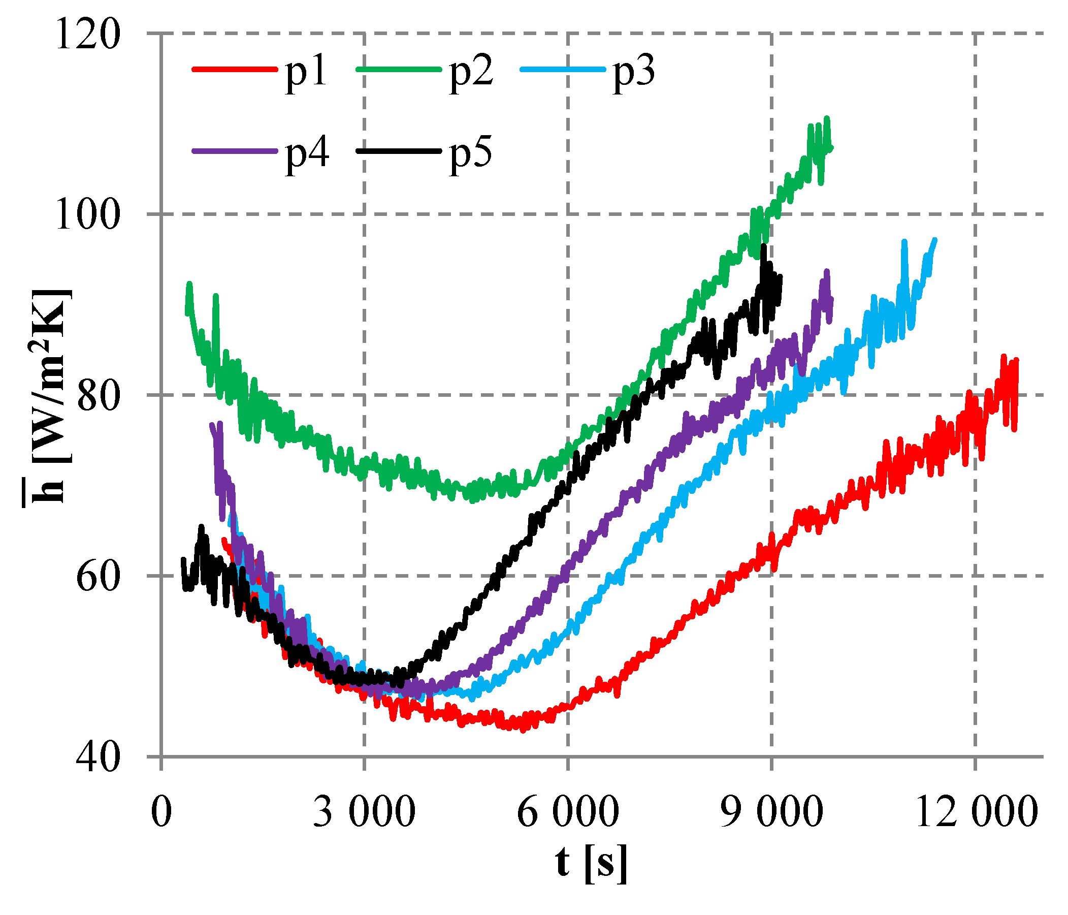
The mean HTC from planes A1–A4 for the time t_k (k = 0, 1, 2, …, N) was calculated based on the following formula:

$$\overline{\mathrm{h}}\left({\mathrm{t}}_{\mathrm{k}}\right)=\frac{1}{4}{\displaystyle \sum }_{\mathrm{i}=1}^4{\mathrm{h}}_{\mathrm{Ai}}\left({\mathrm{t}}_{\mathrm{k}}\right)$$

(9)

Therefore, the mean temperature $\overline{\mathrm{T}}\left(\mathrm{t}\right)$ (8) and mean HTC $\overline{\mathrm{h}}\left(\mathrm{t}\right)$ (9) were functions depending on time. Distribution of these functions for processes p1–p5 is shown in Figure 4 and Figure 5.

Differences between values of temperature and HTC on the cylinder boundary in planes A1, A2, A3 and A4 and respective mean values were considered. To do so, formulae for the absolute difference of temperature (for time t_k, k = 0, 1, 2, …, N)

$$\Delta {\mathrm{T}}_{\mathrm{Ai}}\left({\mathrm{t}}_{\mathrm{k}}\right)={\mathrm{T}}_{\mathrm{Ai}}\left({\mathrm{t}}_{\mathrm{k}}\right)-\overline{\mathrm{T}}\left({\mathrm{t}}_{\mathrm{k}}\right)$$

(10)

and of HTC (for time t_k, k = 0, 1, 2, …, N)

$$\Delta {\mathrm{h}}_{\mathrm{Ai}}\left({\mathrm{t}}_{\mathrm{k}}\right)={\mathrm{h}}_{\mathrm{Ai}}\left({\mathrm{t}}_{\mathrm{k}}\right)-\overline{\mathrm{h}}\left({\mathrm{t}}_{\mathrm{k}}\right)$$

(11)

were used, where i = 1, 2, 3, 4. The relative differences for temperature (for time t_k, k = 0, 1, 2, …, N)

$${\mathsf{\delta }\mathrm{T}}_{\mathrm{Ai}}\left({\mathrm{t}}_{\mathrm{k}}\right)=\frac{{\mathrm{T}}_{\mathrm{Ai}}\left({\mathrm{t}}_{\mathrm{k}}\right)-\overline{\mathrm{T}}\left({\mathrm{t}}_{\mathrm{k}}\right)}{\overline{\mathrm{T}}\left({\mathrm{t}}_{\mathrm{k}}\right)}100\%$$

(12)

and of HTC (for time t_k, k = 0, 1, 2, …, N)

$${\mathsf{\delta }\mathrm{h}}_{\mathrm{Ai}}\left({\mathrm{t}}_{\mathrm{k}}\right)=\frac{{\mathrm{h}}_{\mathrm{Ai}}\left({\mathrm{t}}_{\mathrm{k}}\right)-\overline{\mathrm{h}}\left({\mathrm{t}}_{\mathrm{k}}\right)}{\overline{\mathrm{h}}\left({\mathrm{t}}_{\mathrm{k}}\right)}100\%$$

(13)

were also calculated. The absolute differences of temperature ΔT_Ai(t) (10) and HTC Δh_Ai(t) (11), as well as the relative differences of temperature δT_Ai(t) (12) and HTC δh_Ai(t) (13) (for i = 1, 2, 3, 4), were functions depending on time.

Values described by Formulas (10)–(13) enabled us to compare the boundary condition in the plane Ai (i =1, 2, 3, 4), calculated by solving the inverse problem, and the mean value from the analyzed planes of a given boundary condition in a given time unit. This delivered us information regarding in which part of the furnace the heated element had a temperature or HTC value on the boundary higher or lower than the mean value. It showed in which part of the furnace the process of heat flow from the furnace walls and surrounding gas to the cylinder, being treated thermally and chemically, proceeded more intensively, and in which part it proceeded less intensively. Negative values indicated temperatures and HTC lower than the mean value in a given time unit, while positive values indicated values higher than the mean value. Graphs of the distribution of ΔT_Ai(t) (10), Δh_Ai(t) (11), δT_Ai(t) (12) and δh_Ai(t) (13) in time illustrate the variability of boundary conditions for the heated cylinder during processes of thermo-chemical treatment. A detailed distribution of absolute and relative differences for processes p1 (Figure 6), p2 (Figure 7) and p5 (Figure 8) are presented below. Processes with the same heating speed and various fan set (processes p1 and p2) were chosen to analyze the impact of the gas flow speed on boundary conditions. Moreover, processes with the same fan settings and various heating speeds were also compared (p1 and p5).

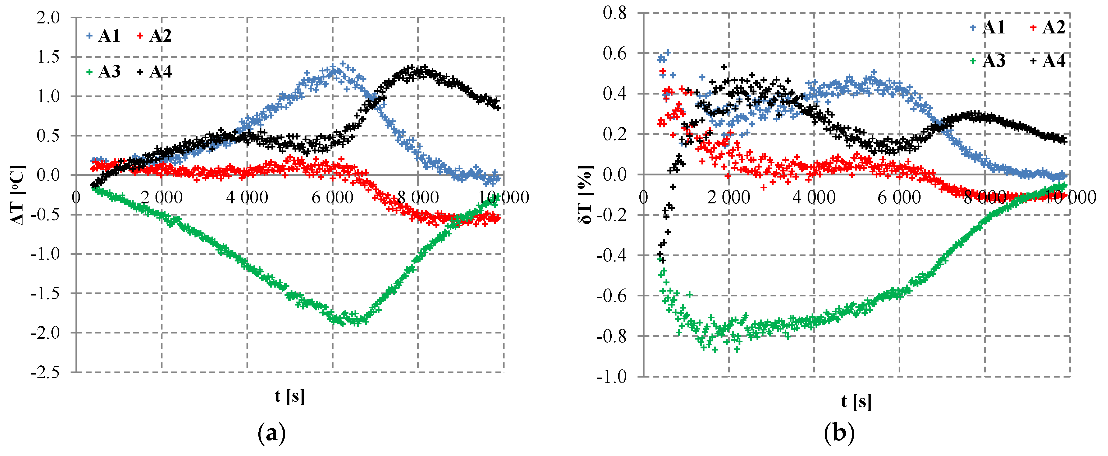
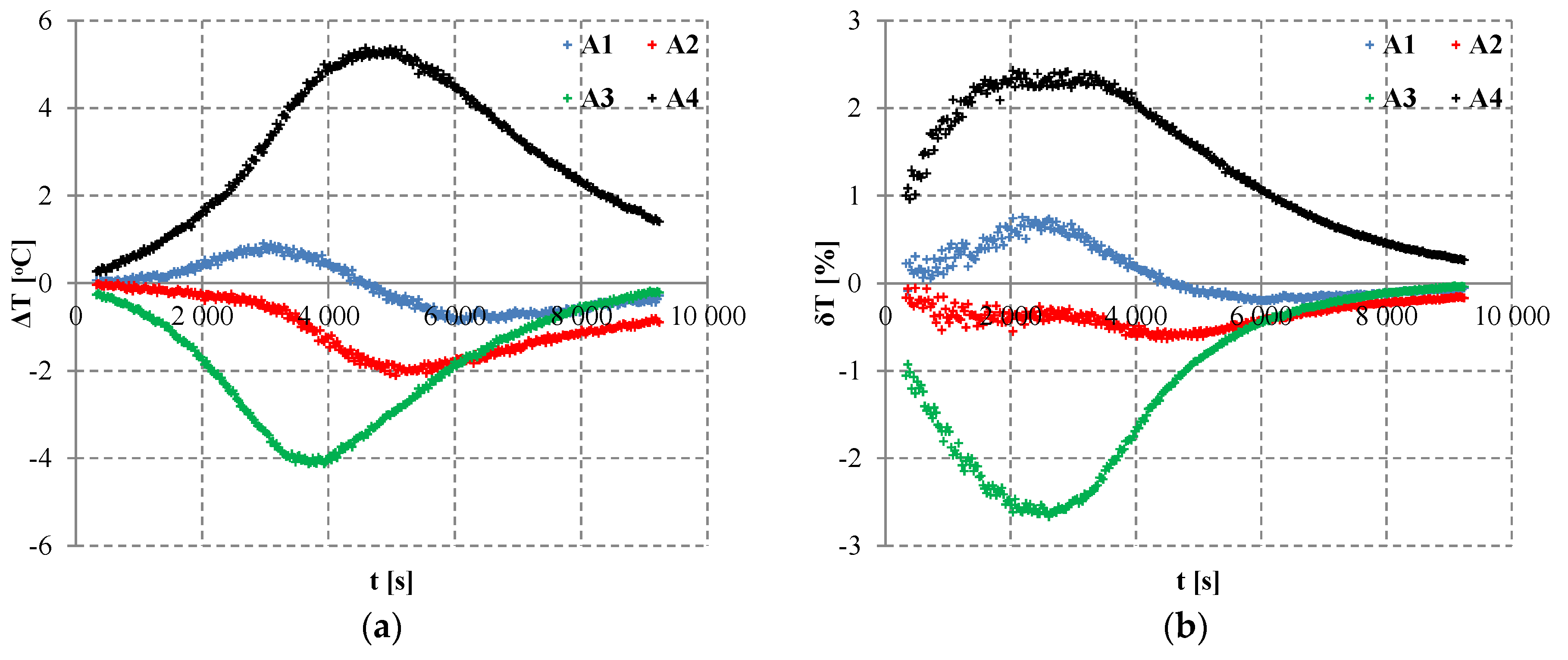
In heating process p1, values of the absolute difference and of the relative difference for temperature in planes A1 and A2 are positive, and in planes A3 and A4, they are negative (Figure 6). This means that in planes A1 and A2, values of temperature on the boundary were higher than the mean value $\overline{\mathrm{T}}\left(\mathrm{t}\right)$ (8), and in planes A3 and A4, they were lower. Based on dependencies from Figure 6, the following estimates for temperature were determined:

Mean value for the absolute difference (10):

$${\mathrm{E}}_1\left(\mathrm{T}\right)=\frac{1}{\mathrm{N}+1}{\displaystyle \sum }_{\mathrm{k}=0}^{\mathrm{N}}\Delta {\mathrm{T}}_{\mathrm{Ai}}\left({\mathrm{t}}_{\mathrm{k}}\right),$$

(14)

Mean value from the absolute value for the absolute difference (10):

$${\mathrm{E}}_2\left(\mathrm{T}\right)=\frac{1}{\mathrm{N}+1}{\displaystyle \sum }_{\mathrm{k}=0}^{\mathrm{N}}\left|\Delta {\mathrm{T}}_{\mathrm{A}\mathrm{i}}\left({\mathrm{t}}_{\mathrm{k}}\right)\right|$$

(15)

Maximum value from the absolute value for the absolute difference (10):

$${\mathrm{E}}_3\left(\mathrm{T}\right)=\underset{0\le \mathrm{k}\le \mathrm{N}}{\max }\left|\Delta {\mathrm{T}}_{\mathrm{Ai}}\left({\mathrm{t}}_{\mathrm{k}}\right)\right|$$

(16)

Mean value for the relative difference (12):

$${\mathrm{E}}_4\left(\mathrm{T}\right)=\frac{1}{\mathrm{N}+1}{\displaystyle \sum }_{\mathrm{k}=0}^{\mathrm{N}}{\mathsf{\delta }\mathrm{T}}_{\mathrm{Ai}}\left({\mathrm{t}}_{\mathrm{k}}\right)$$

(17)

Mean value from the absolute value for the relative difference (12):

$${\mathrm{E}}_5\left(\mathrm{T}\right)=\frac{1}{\mathrm{N}+1}{\displaystyle \sum }_{\mathrm{k}=0}^{\mathrm{N}}\left|{\mathsf{\delta }\mathrm{T}}_{\mathrm{Ai}}\left({\mathrm{t}}_{\mathrm{k}}\right)\right|$$

(18)

and maximum value from the absolute value for the relative difference (12):

$${\mathrm{E}}_6\left(\mathrm{T}\right)=\underset{0\le \mathrm{k}\le \mathrm{N}}{\max }\left|{\mathsf{\delta }\mathrm{T}}_{\mathrm{Ai}}\left({\mathrm{t}}_{\mathrm{k}}\right)\right|$$

(19)

In Formulas (14)–(19), N + 1 denotes the number of time units of the heating process.

Values of estimates E₁–E₆ for temperature (14)–(19) and process p1 are summarized in

Table 4. Values of estimates E₁–E₆ for temperatures (14)–(19) with heating process p1 in planes A1–A4.

	A1	A2	A3	A4
E1 [°C]	1.9	0.9	−1.0	−1.7
E2 [°C]	1.9	0.9	1.0	1.7
E3 [°C]	3.6	1.7	2.2	3.4
E4 [%]	1.2	0.4	−0.6	−1.0
E5 [%]	1.2	0.4	0.6	1.0
E6 [%]	2.4	1.0	1.4	2.8

. The absolute difference in temperature (10) in plane A1 reaches up to 3.6 °C (for time t = 6090 s, Figure 6a, Table 4), and the relative difference (12) is up to 2.4% (Figure 6b, Table 4). In plane A2, these values are up to 1.7 °C for time t = 6660 s and 1%, respectively, at the beginning of the process (Figure 6, Table 4). Relative difference in temperature (12) in plane A2 decreases for subsequent time units. Absolute (10) and relative differences (12) are, respectively, from values close to zero up to –2.2 °C and –1.4% (plane A3) and up to –3.4 °C and –2.8% (plane A4), which is shown in Figure 6 and in Table 4. This means that the temperature along the cylinder length decreases during the process p1. The highest temperature in the cylinder is in the plane located close to the gas stream inflow, and the lowest temperature is in the plane close to the fan.

For process p1, the most intensive heat flow was observed in the area close to the furnace door (plane A1), which was where the direction of gas stream flow was changed. When the gas flowed along the cylinder, it gave its heat to the cylinder; therefore, in the next planes, A2–A4, the temperature on the cylinder boundary became lower and lower. This was proved by the values of estimates E₁ and E₄ (Table 4).

Similar results to those obtained for process p1 (Figure 6, Table 4) were achieved for processes p2 (Figure 7,

Table 5. Values of estimates E₁–E₆ for temperatures (14)–(19) with heating process p2 in planes A1–A4.

	A1	A2	A3	A4
E1 [°C]	0.5	−0.1	−1.0	0.6
E2 [°C]	0.5	0.2	1.0	0.6
E3 [°C]	1.4	0.6	1.9	1.4
E4 [%]	0.3	0.02	−0.5	0.2
E5 [%]	0.3	0.1	0.5	0.3
E6 [%]	0.6	0.5	0.9	0.5

) and p5 (Figure 8,

Table 6. Values of estimates E₁–E₆ for temperature (14)–(19), with heating process p5, in planes A1–A4.

	A1	A2	A3	A4
E1 [°C]	−0.1	−1.0	−1.9	3.0
E2 [°C]	0.5	1.0	1.9	3.0
E3 [°C]	0.9	2.1	4.1	5.4
E4 [%]	0.1	−0.4	−1.2	1.4
E5 [%]	0.2	0.4	1.2	1.4
E6 [%]	0.8	0.6	2.7	2.4

). Process p1 was a reference process for the analysis of processes p2 and p5. In process p2, the heat flow through convection was more intensive than it was in process p1. It resulted from the fan setting, which was 50% of the maximum speed for process p1 and 100% for process p2. In plane A1, values of the absolute and relative difference were positive through most of the process. This meant that temperature in the plane A1 was higher than the mean value. This difference (10) reached up to 1.4 °C (Figure 7a, Table 5). At the end of the process (from time t = 8850 s), these values were negative (Figure 7a). This meant that only at the final stage of the heating process in plane A1 (the closest to the gas stream inflow) was temperature lower than the mean value calculated for the four planes under investigation.

In plane A2, the absolute difference (10) took values from –0.7 °C to 0.2 °C. At the beginning of the heating process, these values were positive, and they decreased in subsequent time units. Relative difference (12) decreased and took values from approximately 0.5 to –0.1%. In reference process p1, these values in planes A1 and A2 were positive for the whole heating process.

In plane A3, the value for temperature was lower than the mean temperature (similarly to process p1). The absolute difference (10) reached up to –1.9 °C (Table 5). Significant differences in temperature courses between processes p1 and p2 were observed in plane A4. The absolute (10) and relative differences in temperature (12) were negative and, respectively, reached up to –3.4 °C and –2.8% for process p1 (Table 4). For process p2, these differences (10) and (12) took positive values. Relative temperature (12) took values up to 0.5% (Figure 7b, Table 5). The absolute difference (10) was 0.6 °C on average and took values from approximately 0.1 °C to 1.4 °C. These dependences indicated the increase of the cylinder temperature in the plane close to the fan, where the gas stream runoff occurred.

For process p2, a significant reduction in the absolute difference (10) and relative difference (12) values was noticeable for the whole time of the heating process when compared with process p1. This meant that the temperature along the cylinder length was more even than in process p1. It resulted from a greater speed of gas flow in the furnace, which was related to more intensive heat flow by convection than in process p1. The maximum speed of the fan caused the intensification of heat flow at the cylinder front (plane A1), resulting from the change in the direction of gas flow in the chamber (similarly to process p1), and at the end part of the cylinder (the plane A4), due to the increasing swirl of gas in the area in front of the fan. It translated to a larger heat flow in plane A4. This was proved by values of the absolute difference (10) and the relative one (12) in plane A4, which were positive for process p2, in contrast to process p1, for which they were negative.

Process p5 was characterized by a higher heating speed when compared with process p1. In plane A1, from the beginning of heating to time t = 4500 s, differences (10) and (12) took positive values, and during the second part of the process, they took negative values (Figure 8, Table 6). In planes A2 and A3, we obtained negative values for the whole time of heating, reaching respectively up to –2.1 °C and –4.1 °C (the absolute difference (10)) and –0.6% and –2.7% (the relative difference (12)), which is shown in Figure 8 and in Table 6. In the middle planes, the temperature during the heating process was lower than its mean value from planes A1–A4. In plane A4 (the closest to the fan), these values were higher, even, by 5.4 °C (Figure 8, Table 6).

In process p5, we observed the highest heating speed of those being investigated (10 °C/min). Increasing the heating speed resulted in an increase of radiation involvement in the heat flow process. Therefore, swirls at the furnace door and in the vicinity of the fan had little impact on arising differences of temperature along the cylinder length. At high heating speeds, the temperature of the internal cylindrical wall of the furnace and temperature of the atmosphere were definitely higher than the temperature of the furnace door becaues there were no heat sources there. That was why the temperature at the front part of the cylinder was not the highest (Figure 7). Gas flowing along the cylinder transferred heat to the cylinder, and at the same time, it heated up from the side walls of the furnace, mainly by radiation. This phenomenon, together with the increase in gas speed in front of the fan, intensified heating of the end part of the cylinder.

During heating processes, in initial time units, the increase of the boundary temperature was slight (about 80 °C within the initial 3000 s or so, Figure 4). It was related to the fact that energy transferred by heat sources caused the increase in temperature of both the cylinder and the whole furnace. In the next stage (from about 3000 to 9000 s or so), the increase in the cylinder boundary temperature was faster (by 400 °C within 6000 s). In the final stage (more than 9000 s), the increase in the cylinder boundary temperature, once again, was slighter, and finally it passed to the soaking phase. At the beginning of the process, temperature in the cylinder was constant. With passing time, the unevenness of heating increased. Next, values of the absolute differences in temperature ΔT (10) were positive in planes with temperatures higher than the mean and negative in planes with temperatures lower than the mean (Figure 6, Figure 7 and Figure 8). Values of the absolute difference (10) diverged the most from zero during the stage of fast increase in the cylinder temperature (from 3000 to 9000 s), when the unevenness of heating in the furnace for thermo-chemical treatment was the greatest (Figure 6a, Figure 7a and Figure 8a). Values ΔT (10) were much closer to zero at the beginning and at the end of processes p1–p5, when the heating process started (up to 3000 s) and when parameters of furnace operation approached the soaking phase (more than 9000 s). The values of temperatures of the cylinder boundary were obtained based on the solution of the inverse problem, which was numerically ill-conditioned. It meant that a slight disturbance to input data could cause a significant disturbance to the results. Therefore, a regularization of the solution to the inverse problem was needed. For the problem considered herein, the time step regularization method was applied. This method had been already tested, which was described in paper [19]. For non-stationary problems, oscillations of the solution in the initial time units were characteristic. 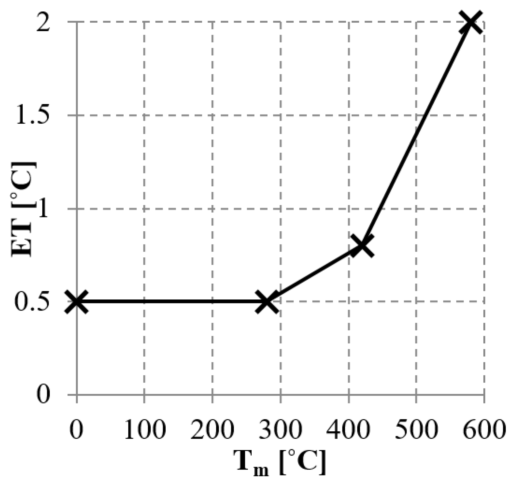Therefore, results (Figure 4, Figure 5, Figure 6, Figure 7, Figure 8 and Figure 9) are not shown from time t = 0. Taking into consideration the accuracy of temperature measurement (Figure 2), results for initial time units were rejected. Similarly, for the final stage before soaking, when the increase in the boundary temperature was slight, significant oscillations of the solution to the inverse problem occurred. They resulted from ill conditioning of the inverse problem and small differences in temperature at measuring points in the cylinder and small differences in temperature between the gas and the cylinder boundary. Based on the analysis of errors for processes p1–p5, such time intervals were selected for which results of the solution to the inverse problem were obtained with permissible accuracy (Table 3). The absolute differences for temperature ΔT (10) for the last time unit were within the range of −1.2 to 0.8 °C for process p1 (Figure 6a), of −0.5 to 0.8 °C for process p2 (Figure 7a) and of −0.9 to 1.4 °C for process p5 (Figure 8a). Values ΔT (10) went to zero, which indicated a reduction in the unevenness of the cylinder heating in the final stages of the processes. However, they did not achieve the zero value because differences in temperature in the cylinder still occurred. For process p2, where the unevenness of heating was the smallest due to the greater involvement of convection (100% of fan speed), the reliability of the results of the solution to the inverse problem was up to time t = 9870 s. Values ΔT (10) at the final phase of process p2 were the closest to zero when compared with the other processes under consideration (Figure 6a, Figure 7a and Figure 8a). However, the character of the absolute difference (10) course close to the fan (plane A4) in process p2 was slightly different than in processes p1 and p5. It resulted from a more intensive heat flow close to the fan.

Values of the estimates for process p3 are summarized in

Table 7. Values of estimates E₁–E₆ for temperatures (14)–(19), with heating process p3, in planes A1–A4.

	A1	A2	A3	A4
E1 [°C]	−0.1	−1.0	−1.7	2.7
E2 [°C]	0.5	1.0	1.7	2.7
E3 [°C]	0.9	1.9	3.7	5.0
E4 [%]	0.1	−0.3	−1.0	1.2
E5 [%]	0.2	0.3	1.0	1.2
E6 [%]	0.6	0.5	2.0	1.9

, and for process p4, in

Table 8. Values of estimates E₁–E₆ for temperatures (14)–(19), with heating process p4, in planes A1–A4.

	A1	A2	A3	A4
E1 [°C]	−0.1	−1.0	−1.9	3.0
E2 [°C]	0.5	1.0	1.9	3.0
E3 [°C]	0.9	1.9	4.1	5.2
E4 [%]	0.1	−0.3	−1.2	1.4
E5 [%]	0.3	0.3	1.2	1.4
E6 [%]	0.8	0.5	2.6	2.3

.

The greatest differences in temperature along the cylinder length (T_max–T_min achieved the maximum value) in processes p1–p5 were obtained at the times summarized in

Table 9. Times at which the greatest differences in temperature values along the cylinder length occurred.

	p1	p2	p3	p4	p5
t [s]	6600	6240	6060	4950	3930

. This difference for process p1 was 6.8 °C (

Table 10. Temperatures in planes A1, A2, A3 and A4 at the time at which the greatest differences in temperature values along the cylinder length occurred.

Process	p1	p2	p3	p4	p5
plane	T [°C]
A1	293.4	329.7	309.7	275.7	231.1
A2	291.5	328.4	308.4	274	229.3
A3	288	326.4	306.3	271.6	226.5
A4	286.6	328.7	314.5	280.4	235.6
Tmax–Tmin	6.8	3.3	8.2	8.8	9.1

). Increasing the number of revolutions of the fan resulted in more intensive heat flow by convection, and in consequence, in reducing the temperature difference along the cylinder length to 3.3 °C (Table 10). On the other hand, increasing the speed of heating resulted in more intensive heat flow by radiation and the increase of maximum differences in temperature between planes to values of 8.2, 8.8 and 9.1 °C, respectively, for processes p3, p4 and p5.

For HTC, values of estimates E₁–E₆ were determined according to the following formulae:

$${\mathrm{E}}_1\left(\mathrm{h}\right)=\frac{1}{\mathrm{N}+1}{\displaystyle \sum }_{\mathrm{k}=0}^{\mathrm{N}}\Delta {\mathrm{h}}_{\mathrm{Ai}}\left({\mathrm{t}}_{\mathrm{k}}\right)$$

(20)

$${\mathrm{E}}_2\left(\mathrm{h}\right)=\frac{1}{\mathrm{N}+1}{{\displaystyle \sum }}_{\mathrm{k}=0}^{\mathrm{N}}\left|\Delta {\mathrm{h}}_{\mathrm{Ai}}\left({\mathrm{t}}_{\mathrm{k}}\right)\right|$$

(21)

$${\mathrm{E}}_3\left(\mathrm{h}\right)=\underset{0\le \mathrm{k}\le \mathrm{N}}{\max }\left|\Delta {\mathrm{h}}_{\mathrm{Ai}}\left({\mathrm{t}}_{\mathrm{k}}\right)\right|$$

(22)

$${\mathrm{E}}_4\left(\mathrm{h}\right)=\frac{1}{\mathrm{N}+1}{\displaystyle \sum }_{\mathrm{k}=0}^{\mathrm{N}}{\mathsf{\delta }\mathrm{h}}_{\mathrm{Ai}}\left({\mathrm{t}}_{\mathrm{k}}\right)$$

(23)

$${\mathrm{E}}_5\left(\mathrm{h}\right)=\frac{1}{\mathrm{N}+1}{\displaystyle \sum }_{\mathrm{k}=0}^{\mathrm{N}}\left|{\mathsf{\delta }\mathrm{h}}_{\mathrm{Ai}}\left({\mathrm{t}}_{\mathrm{k}}\right)\right|$$

(24)

$${\mathrm{E}}_6\left(\mathrm{h}\right)=\underset{0\le \mathrm{k}\le \mathrm{N}}{\max }\left|{\mathsf{\delta }\mathrm{h}}_{\mathrm{Ai}}\left({\mathrm{t}}_{\mathrm{k}}\right)\right|.$$

(25)

In Formulas (20)–(25), N + 1 denotes the number of time units of the heating process.

Values of estimates E₁–E₆ for HTC (20)–(25) and process p1 are summarized in

Table 11. Values of estimates E₁–E₆ for HTC (20)–(25) with heating process p1 in planes A1–A4.

HTC	A1	A2	A3	A4
E1 [W/m2K]	1.3	0.9	−0.6	−1.6
E2 [W/m2K]	1.9	1.5	1.4	1.9
E3 [W/m2K]	9.0	9.1	8.8	14.4
E4 [%]	2.5	1.5	−1.3	−2.7
E5 [%]	3.4	2.6	2.4	3.3
E6 [%]	16.1	15.4	12.7	22.5

. Results similar to those from process p1 (Table 11) were obtained for processes p2 (

Table 12. Values of estimates E₁–E₆ for HTC (20)–(25) with heating process p2 in planes A1–A4.

HTC	A1	A2	A3	A4
E1 [W/m2K]	0.5	−0.3	−1.2	1.0
E2 [W/m2K]	1.8	1.6	1.6	1.9
E3 [W/m2K]	10.6	8.2	6.3	9.8
E4 [%]	0.6	−0.3	−1.5	1.1
E5 [%]	2.2	2.0	2.0	2.4
E6 [%]	12.5	10.1	7.7	11.0

) and p5 (

Table 13. Values of estimates E₁–E₆ for HTC (20)–(25) with heating process p5 in planes A1–A4.

HTC	A1	A2	A3	A4
E1 [W/m2K]	−0.2	−0.9	−1.1	2.3
E2 [W/m2K]	1.5	1.6	1.7	2.5
E3 [W/m2K]	10.6	9.5	7.4	10.0
E4 [%]	−0.2	−1.3	−2.1	3.6
E5 [%]	2.2	2.4	2.8	3.9
E6 [%]	18.0	11.1	12.2	16.9

).

The absolute difference of HTC (11) in process p1 was the greatest for plane A4 and reached the value of 14.4 W/m²K. For other planes, it reached approximately 9 W/m²K (Table 11). The relative difference (13) reached values up to 22.5% (plane A4). HTC values in planes A1 and A2 were higher than the mean value, and in planes A3 and A4, they were lower, which was proved by the values of estimates E1 and E4. These values resulted from heating the cylinder wall at the inflow side.

Changes to the fan setting affected HTC values, which, on average, took values lower than $\overline{h}$ in planes A2 and A3 and higher in planes A1 and A4. This meant more intensive heat flow at the cylinder ends. The absolute difference (11) reached up to 10.6, 8.2, 6.3 and 9.8 W/m²K respectively for planes A1–A4.

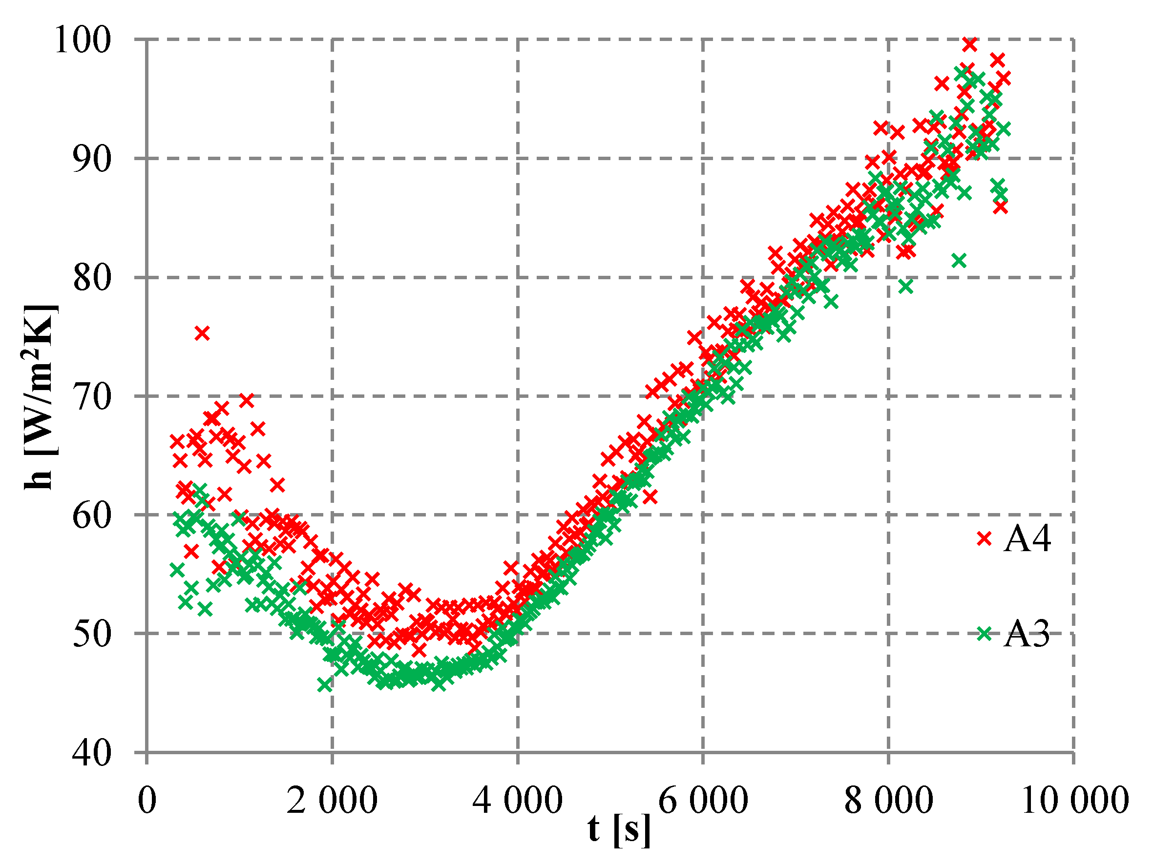
In process p5, the absolute (11) and relative differences (13), on average, took negative value in planes A1–A3 and a positive value in plane A4. It meant that at the ending part of the cylinder, the heat flow was intensified by gas backward swirl generated by the fan blades’ movements (estimates E₁ (20) and E₄ (23)). The difference between the HTC mean value and its value (11) in plane A1 reached up to 10.6 W/m²K. For other planes, these values were slightly lower and reached up to 10.0 (plane A4), 9.5 (plane A2) and 7.4 W/m²K (plane A3). The illustrative course of HTC in planes A3 and A4 for process p5 is presented in Figure 9.

Values of estimates E₁–E₆ for HTC (20)–(25) and process p3 are summarized in

Table 14. Values of estimates E₁–E₆ for HTC (20)–(25) with heating process p3 in planes A1–A4.

HTC	A1	A2	A3	A4
E1 [W/m2K]	−0.1	−1.1	−1.0	2.2
E2 [W/m2K]	1.6	1.7	1.7	2.4
E3 [W/m2K]	10.0	10.5	9.1	10.6
E4 [%]	−0.1	−1.5	−2.0	3.6
E5 [%]	2.4	2.5	2.7	3.9
E6 [%]	10.9	11.9	11.3	16.5

and for the process p4, in

Table 15. Values of estimates E₁–E₆ for HTC (20)–(25) with heating process p4 in planes A1–A4.

HTC	A1	A2	A3	A4
E1 [W/m2K]	−0.1	−0.9	−1.2	2.2
E2 [W/m2K]	1.4	1.5	1.7	2.4
E3 [W/m2K]	8.4	9.5	9.2	11.4
E4 [%]	−0.1	−1.4	−2.2	3.6
E5 [%]	2.1	2.3	2.8	3.9
E6 [%]	10.1	10.6	12.0	16.8

.

5. Conclusions

This paper presented research on changes in thermodynamic parameters in the chamber of a furnace for thermo-chemical treatment. Values of temperature and HTC on the cylinder boundary were calculated along the cylinder length in four planes. The greatest deviation from the mean value of temperature was obtained for process p5 in plane A4. It was 5.4 °C (estimate E₃ (16)). Changes in the fan setting reduced temperature differences on the cylinder boundary from 6.8 (process p1) to 3.3 °C (process p2). Differences in temperature on the cylinder boundary could reach values above 9 °C for process p5 with the maximum heating speed. At that point, the greatest unevenness of the cylinder heating was observed. Results included in this paper indicate that during heating, significant changes of temperature may occur in elements being heated depending on their location. The mean deviation of HTC from the mean value is the greatest close to the fan (plane A4, estimate E₂ (21)) for all heating processes, and it does not exceed 2.46 W/m²K, whereas the the maximum deviation of HTC in plane A4 from the mean value reaches up to −14.4 W/m²K (process p1) and 11.4 W/m²K (process p4). The course of obtained HTC curves in different planes along the cylinder length is similar over time.

Knowledge of temperature on the cylinder boundary, HTC and unevenness of these boundary conditions along the cylinder length for various heating speeds and fan settings is very important for processes of thermo-chemical treatment. It can be the basis for making a decision regarding at what furnace setting the charge should be heated and when gases such as ammonia for nitriding should be applied. Furnace settings affect the time of heating and the differences in temperature arising in the element being heated, which can produce thermal stresses. Calculated boundary conditions provide the basis for investigation of the process of creating surface layers with structures correlated with temperature. Therefore, boundary conditions, determined by solving the inverse problem, can constitute the basis for optimizing the processes of thermo-chemical treatment.

References

1. Alifanov, O.M. Inverse Heat Transfer Problems; Springer: Berlin, Germany, 1994. [Google Scholar]
2. Jaremkiewicz, M.; Taler, J. Online Determining Heat Transfer Coefficient for Monitoring Transient Thermal Stresses. Energies 2020, 13, 704. [Google Scholar] [CrossRef] [Green Version]
3. Joachimiak, M.; Ciałkowski, M. Stable solution to nonstationary inverse heat conduction equation. Arch. Thermodyn. 2018, 39, 25–37. [Google Scholar] [CrossRef]
4. Joachimiak, D.; Krzyślak, P. Comparison of results of experimental research with numerical calculations of a model one-sided seal. Arch. Thermodyn. 2015, 36, 61–74. [Google Scholar] [CrossRef]
5. Hadamard, J. Sur les Problèmes aux Dérivéespartielles et leur Signification Physique; Princeton Univ. Bull.: Princeton, NJ, USA, 1902; pp. 49–52. [Google Scholar]
6. Cao, K.; Lesnic, D.; Liu, J. Simultaneous reconstruction of space-dependent heat transfer coefficients and initial temperature. J. Comput. Appl. Math. 2020, 375, 112800. [Google Scholar] [CrossRef]
7. Frąckowiak, A.; Olejnik, A.; Wróblewska, A.; Ciałkowski, M. Application of the Protective Coating for Blade’s Thermal Protection. Energies 2021, 14, 50. [Google Scholar] [CrossRef]
8. Grysa, K.; Maciag, A.; Cebo-Rudnicka, A.; Walaszczyk, M. Identification of the heat transfer coefficient during cooling proces by means of Trefftz method. Eng. Anal. Bound. Elem. 2018, 95, 33–39. [Google Scholar] [CrossRef]
9. Joachimiak, D.; Frąckowiak, A. Experimental and numerical analysis of the gas flow in the axisymmetric radial clearance. Energies 2020, 13, 5794. [Google Scholar] [CrossRef]
10. Joachimiak, D.; Krzyślak, P. Analysis of the Gas Flow in a Labyrinth Seal of Variable Pitch. J. Appl. Fluid Mech. 2019, 12, 921–930. [Google Scholar] [CrossRef]
11. Joachimiak, D.; Krzyślak, P. Experimental research and CFD calculations based investigations into gas flow in a short segment of a heavily worn straight through labyrinth seal. Pol. Marit. Res. 2017, 24, 83–88. [Google Scholar] [CrossRef] [Green Version]
12. Joachimiak, M.; Ciałkowski, M.; Frąckowiak, A. Stable method for solving the Cauchy problem with the use of Chebyshev polynomials. Int. J. Numer. Methods Heat Fluid Flow 2020, 30, 1441–1456. [Google Scholar] [CrossRef]
13. da Silva, W.B.; Dutra, J.C.S.; Kopperschimidt, C.E.P.; Lesnic, D.; Aykroyd, R.G. Sequential particle filter estimation of a time-dependent heat transfer coefficient in a multidimensional nonlinear inverse heat conduction problem. Appl. Math. Model. 2021, 89, 654–668. [Google Scholar] [CrossRef]
14. Ciałkowski, M.; Olejnik, A.; Frąckowiak, A.; Lewandowska, N.; Mosiężny, J. Cauchy type inverse problem in a two-layer area in the blades of gas turbine. Energy 2020, 212, 118751. [Google Scholar]
15. Joachimiak, M. Choice of the regularization parameter for the Cauchy problem for the Laplace equation. Int. J. Numer. Methods Heat Fluid Flow 2020, 30, 4475–4492. [Google Scholar] [CrossRef]
16. Marin, L. Landweber–Fridman algorithms for the Cauchy problem in steady-state anisotropic heat conduction. Math. Mech. Solids 2020, 25, 1340–1363. [Google Scholar] [CrossRef]
17. Lee, S.-Y.; Yan, Q.-Z. Inverse analysis of heat conduction problems with relatively long heat treatment. Int. J. Heat Mass Transf. 2017, 105, 401–410. [Google Scholar] [CrossRef]
18. Murzin, S.P.; Bielak, R.; Liedl, G. Algorithm for calculation of the power density distribution of the laser beam to create a desired thermal effect on technological objects. Comput. Opt. 2016, 40, 679–684. [Google Scholar] [CrossRef]
19. Joachimiak, M.; Joachimiak, D.; Ciałkowski, M.; Małdziński, L.; Okoniewicz, P.; Ostrowska, K. Analysis of the heat transfer for processes of the cylinder heating in the heat-treating furnace on the basis of solving the inverse problem. Int. J. Thermal Sci. 2019, 145, 105985. [Google Scholar] [CrossRef]
20. Jaremkiewicz, M.; Taler, D.; Dzierwa, P.; Taler, J. Determination of Transient Fluid Temperature and Thermal Stresses in Pressure Thick-Walled Elements Using a New Design Thermometer. Energies 2019, 12, 222. [Google Scholar] [CrossRef] [Green Version]
21. Taler, D.; Sobota, T.; Jaremkiewicz, M.; Taler, J. Influence of the Thermometer Inertia on the Quality of Temperature Control in a Hot Liquid Tank Heated with Electric Energy. Energies 2020, 13, 4039. [Google Scholar] [CrossRef]
22. Kurc, B.; Lijewski, P.; Rymaniak, Ł.; Fuć, P.; Pigłowska, M.; Urbaniak, R.; Ciupek, B. High-Energy Solid Fuel Obtained from Carbonized Rice Starch. Energies 2020, 13, 4096. [Google Scholar] [CrossRef]
23. Lakatos, Á.; Csík, A.; Csarnovics, I. Experimental verification of thermal properties of the aerogel blanket. Case Studies Thermal Eng. 2021, 25, 100966. [Google Scholar] [CrossRef]
24. Zhang, A.; Liang, S.; Guo, Z.; Xiong, S. Determination of the interfacial heat transfer coefficient at the metal-sand mold interface in low pressure sand casting. Exp. Therm. Fluid Sci. 2017, 88, 472–482. [Google Scholar] [CrossRef]
25. Judt, W. Numerical and Experimental Analysis of Heat Transfer for Solid Fuels Combustion in Fixed Bed Conditions. Energies 2020, 13, 6141. [Google Scholar] [CrossRef]
26. Maciejewska, B.; Strak, K.; Piasecka, M. The solution of a two-dimensional inverse heat transfer problem using two methods: The Trefftz method and the Beck method. Int. J. Numer. Methods Heat Fluid Flow 2018, 28, 206–219. [Google Scholar] [CrossRef]
27. Hożejowska, S.; Piasecka, M. Numerical Solution of Axisymmetric Inverse Heat Conduction Problem by the Trefftz Method. Energies 2020, 13, 705. [Google Scholar] [CrossRef] [Green Version]
28. Piasecka, M.; Hożejowska, S.; Maciejewska, B.; Pawińska, A. Time-Dependent Heat Transfer Calculations with Trefftz and Picard Methods for Flow Boiling in a Mini-Channel Heat Sink. Energies 2021, 14, 1832. [Google Scholar] [CrossRef]
29. Frąckowiak, A.; Spura, D.; Gampe, U.; Ciałkowski, M. Determination of heat transfer coefficient in a T-shaped cavity by means of solving the inverse heat conduction problem. Int. J. Numer. Methods Heat Fluid Flow 2019, 30, 1725–1742. [Google Scholar] [CrossRef]
30. Paszkowski, S. Numerical Application of Multinomials and Chebyshev Series; PWN: Warsaw, Poland, 1975. (In Polish) [Google Scholar]
31. Joachimiak, M.; Ciałkowski, M. Non-linear unsteady inverse boundary problem for heat conduction equation. Arch. Thermodyn. 2017, 38, 81–100. [Google Scholar] [CrossRef] [Green Version]
Figure 1. Working chamber of the furnace with cylinder view from the furnace’s door (a) and diagram of the furnace: 1—working chamber of the furnace, 2—fan, 3—annular channel, 4—door, 5—heat source, 6—wall of working chamber, 7—cylindrical partition, 8—cylinder with marked measuring planes A1–A4 and the gas flow direction (b).
Energies 14 02903 g001
Figure 2. The course of the error in temperature measurement ET, depending on the measured temperature.
Energies 14 02903 g002
Figure 3. Scheme of the calculation procedure for tk-th time unit.
Energies 14 02903 g003
Figure 4. Mean value of temperatures on the cylinder boundary (for planes A1–A4) for processes p1–p5.
Energies 14 02903 g004
Figure 5. Mean values of HTC on the cylinder boundary (for planes A1–A4) for processes p1–p5.
Energies 14 02903 g005
Figure 6. Course of the absolute difference (a) and of the relative difference (b) for temperature and process p1 in planes A1, A2, A3 and A4.
Energies 14 02903 g006
Figure 7. Course of the absolute difference (a) and of the relative difference (b) for temperature and process p2 in planes A1, A2, A3 and A4.
Energies 14 02903 g007
Figure 8. Course of the absolute difference (a) and of the relative difference (b) for temperature and process p5 in planes A1, A2, A3 and A4.
Energies 14 02903 g008
Figure 9. HTC in planes A3 and A4 for process p5.
Energies 14 02903 g009