Numerical modelling is a powerful tool to deal with the complex phenomenon of hydraulic fracturing. FLAC3D (fast Lagrangian analysis of continua in 3D) is a numerical modeling software which utilizes an explicit finite volume method to solve a wide variety of geotechnical problems [
30]. Since FLAC3D deals with continuum mechanics, a new numerical 3D-model built on tensile fracture (discontinuous media) criterion in the presence of 3D stress state and hydromechanical coupling between fracture and matrix was developed by Zhou and Hou [
31]. The effects of stress redistribution after the tensile failure and fluid leakoff to the matrix were all numerically modelled. To simulate proppant transport with gelled fluid, the solid-liquid two phase flow in the fracture was integrated, including proppant concentration, shear rate, fluid viscosity, proppant, and fluid densities, etc. [
32]. These models were integrated into FLAC3D. The effect of reservoir heterogeneity on fracture orientation was also investigated in tight gas reservoirs using XFEM and FVM approaches [
33]. To numerically study the heat transport in the fracture and heat exchange between the fracture and formation, a new thermal module was added to FLAC3D [
34]. To model the THM processes in an MM environment, two well established numerical simulators, FLAC3D and TOUGH2, were coupled to exchange data with non-linear coupling functions [
35,
36,
37]. The in-house upgraded version of FLAC3D, called FLAC3D
plus, was then coupled with TOUGH2MP to model hydraulic fracturing in different reservoirs such as oil, gas, and geothermal [
37,
38,
39,
40].
To simulate the hydraulic fracturing with n-heptane, it is important to model its behavior in the presence of formation fluids, i.e., water and gas. In addition, the determination of properties such as viscosity, density, and enthalpy, etc., of an alternative fluid at reservoir conditions is also imperative to properly understand its performance. Therefore, there is a need for a three-phase multi-component model which can simulate the flow of n-heptane as a separate phase in a non-isothermal environment. TMVOC (belonging to the family of TOUGH2) can model the MM flow of volatile organic chemicals in a non-isothermal manner [
41]. Parameters such as saturation, relative permeability, viscosity, density, specific enthalpy, capillary pressure, and diffusion for every phase are considered and updated at each successful Newton-Raphson iteration. Hence, the appearance and disappearance of phases and components in different phases is modeled with reasonable accuracy.
Thus, numerical modeling of hydraulic fracturing with a variety of fluids (alternative and conventional) can be performed by coupling FLAC3D
plus (full 3D rock mechanical simulator) and TMVOC (reservoir simulator). In this approach, a fracture model, MM fluid flow model, and proppant transport model are implemented in the THM coupled FLAC3D
plus-TMVOC framework [
38,
39]. In addition, fracture elements residing in the host matrix elements in a pre-defined path perpendicular to least principal stress are considered.
2.2.1. Mechanical Deformation
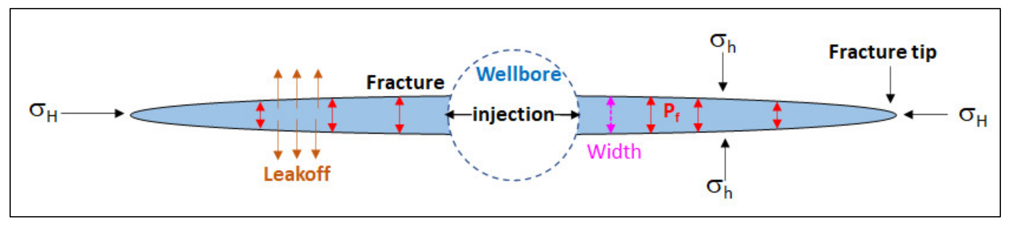
The main formulation utilized for mechanical calculations is based on FLAC3D. However, as the fracture is a discontinuous media, the discontinuous displacement due to tensile failure needed to be modelled. The flow in the fracture can be considered between two parallel plates. Continued injection of fluid after fracture initiation leads to the leakoff of fluid into the formation matrix from the fracture. Consequently, the pressure in the fracture changes. A simple bi-wing fracture can be observed in
Figure 4.
In order to perform the mechanical calculations, FLAC3D
plus formulation, which relies upon the elasto-plasticity theory, is used. In this regard, the displacement increment in a time interval is determined by the solution of the equation of motion (Equation (1)). The strain and stress increments in a time step can be determined using the continuum and constitutive equations (Equations (2) and (3)) [
30].
where,
(considering compressive stress positive);
: stress (Pa);
: effective stress (Pa);
: Biot’s-coefficient (-);
: reservoir pressure (Pa);
: density (kg/m
3);
: gravitational acceleration (m/s
2);
: velocity (m/s);
: time (s);
: strain increment (-);
: displacement (m)
: effective stress increment;
: physical matrix;
: Poisson coefficient (-);
: Elastic modulus (Pa);
: Poisson’s ratio (-); and
.
The tensile failure of the rock occurs when the injected fluid pressure exceeds the combined effect of the smallest principal stress and tensile strength. The fracture propagates in the path of least resistance, which is perpendicular to the least principal stress. Considering compressive stress to be positive, the failure criteria can be described as [
31,
32,
42]:
: minimum principal stress (Pa);
: tensile strength of rock (Pa); and
: pressure in fracture (Pa).
Due to the fluid injection, the pressure inside the fracture changes, effectuating the deformation of fracture elements. Hence, strain change perpendicular to fracture is induced. This strain increment is dependent upon the pressure inside the fracture working against the normal compressive stress, which is mathematically expressed by Equation (5):
The fracture width increment due to strain change, considering the small width of the host element, is calculated as follows:
where
: strain increment (-);
(rock toughness);
: pressure at new time step (Pa);
: normal stress at previous time step {Pa);
: bulk modulus of rock (Pa);
: shear modulus (Pa);
: fracture width change (m); and
: width of the zone perpendicular to fracture (m).
Injection pressure that is higher than the closure stress gives rise to width augmentation. However, as the fluid injection is stopped, the pressure inside the fracture decreases and the fluid leaks off to the formation, resulting in width reduction. To avoid complete fracture closure, proppants are injected which keep the fracture open. This requires the inclusion of contact stress in the strain increment Equation (5), which is written as:
where,
: proppant concentration (m
3/m
3);
: over reduced strain (-); and
: residual width (m).
The fracture propagation in this model utilizes the concept of subdividing the zones into fractured, partially fractured, and unfractured elements. The zone containing the fracture tip is crucial and is therefore further divided into sub-elements to enhance the precision of numerical modeling (
Figure 5) [
43]. Once enough sub-elements are fractured in an element, its status is changed to fractured element and the next element becomes the tip or partially fractured element. The zones beyond the fracture tip are considered unfractured.
2.2.2. Multi-phase Multi-Component (MM) Fluid Flow and Proppant Transport
For the MM flow of fluid in the fracture and matrix, TMVOC formulation is utilized [
41]. The mass conservation for different components and phases is given as:
: mass accumulation term for component k (mol/m
3);
: mass flux (mol/m
2/s);
: liquid/gas/NAPL (non-aqueous phase liquids) phase;
: component
k mole fraction in phase
β (-); and
: source or sink (mol/m
3/s).
Solving the MM flow problem requires space discretization. A model is divided into small discrete blocks and the integral finite difference method is used for averaging. A discrete volume element (
Vn) in the system is shown in
Figure 6, bounded by the closed surface
Γn. The interface area between blocks is represented by A (
Figure 6). Then, surface integrals for mass or energy can be approximated by taking the integral of Equation (8).
The mass of a component k includes its share from all the phases in which it is present. Mass accumulation for the formation (matrix) for different phases in the reservoir is based upon the following relation:
where
: porosity (-);
: saturation of phase
(-); and
: density of phase
(mol/m
3).
The flow simulation can be characterized into three categories, which include flow in fracture, flow between fracture and matrix, and matrix flow. The discrete elements are subdivided into matrix or reservoir elements and potential fracture elements. Darcy law governs the fluid flow in these elements, which can be written for a fluid phase
β as:
: Darcy velocity (m/s);
: permeability (m
2);
: relative permeability of phase β;
: viscosity of phase
β (Pa·s);
: pressure gradient (Pa/m); and
: gravity (m/s
2).
Due to hydraulic fracturing, a fracture with a certain width is present. Therefore, the mass conservation equation for a fracture involves the inclusion of fracture width to Equation (8), given by:
where,
: fraction of fractured sub-element:
(-); and
: fracture width (m).
Fluid viscosity determination is of prime importance for determining the fluid flow behavior in porous media. During the hydraulic fracturing operation, the fluid viscosity is affected by gelling, proppant transport, shear and, especially, temperature variations. For mixture viscosity, the following relation is utilized in TMVOC:
: viscosity of NAPL phase (Pa·s);
: viscosity of component
k in NAPL mixture (Pa·s); and
: mole fraction of component
k in NAPL phase.
For proppant transport and avoiding unnecessary fluid loss, fluids are normally gelled using guar gum. During the fracturing and proppant transport process, the fluid viscosity varies, accordingly the term apparent fluid viscosity is used which depends upon the shear rate, proppant concentration, and temperature differentials, etc. The following relations modified from Torres et al. and Zhang et al. [
44,
45] are utilized for apparent viscosity to include the effect of shear rate, gelling agent concentration, and temperature variations:
where,
: apparent viscosity (Pa·s);
: zero shear viscosity (Pa·s);
: apparent shear rate (1/s);
: flow index;
: constants (-);
: guar concentration (g/l)
: activation energy of viscous flow (J/mol);
: ideal gas constant (J/mol/K)
: temperature (K); and
: reference temperature (K).
Once the proppant injection starts, the viscosity of the proppant-carrying slurry changes. Barre and Conway [
46] presented the following correlation to include the effect of proppant concentration on fluid viscosity:
: proppant concentration in the slurry (-);
: maximum proppant concentration (-); and
a: correlation coefficient.
To model the fluid flow including the effect of shear, temperature variation, gelling agent concentration, and proppant concentration on viscosity, the above equations are combined to give the new model as given by Equation (17) [
41,
44,
45]:
where
: apparent viscosity of proppant carrying fluid (component k) in the NAPL phase.
The proppant-carrying slurry velocity and proppant settling velocity is found by the following set of equations [
32]:
where
: proppant carrying slurry velocity (m/s);
: proppant concentration (-);
: fluid velocity (m/s);
: proppant velocity (m/s);
: proppant settling velocity (m/s);
: proppant density (kg/m
3);
: fluid density (kg/m
3);
: apparent viscosity (Pa·s); and
: particle Reynold’s number:
.
The injection of NAPL (n-heptane or other hydrocarbons) into a gas reservoir in the presence of connate water requires three-phase fluid modeling. To model the multi-phase flow, a modified version of Stone’s three-phase relative permeability function (available in TMVOC) is applied as defined by the following equations [
41,
47]:
The injected fluid saturation is found as and : gas phase relative permeability (-); : water phase relative permeability (-); : NAPL (alkane: n-heptane) phase relative permeability (-); : gas phase saturation (-); : water phase saturation (-); : NAPL (n-heptane) saturation (-); : irreducible gas saturation (-); : irreducible water saturation (-); and : irreducible NAPL (n-heptane) saturation (-).
Moreover, the three-phase capillary function from Parker et al. [
48] is used in the TMVOC for measuring the capillary pressure given by the following relations [
41]:
where
,
,
,
: capillary pressure gas-alkane (n-heptane), and
: capillary pressure gas-water.
The fracturing, fluid flow and proppant transport models are implemented in the FLAC3D
plus-TMVOC coupling. The data sharing between software and specific calculations performed at a time step can be observed in detail in
Figure 7. The computing time of the simulation depends upon the size of 3D model, number of grid blocks, isothermal or non-isothermal process, number of components for injection and production, etc., and therefore may range from a few hours to a few days.


 ,
, 


