Article

Efficient Operation Method of Aquifer Thermal Energy Storage System Using Demand Response

1
Artificial Intelligence Applied Research Institute, Kurume Institute of Technology, 2228-66 Kamitsu-machi, Kurume, Fukuoka 830-0052, Japan
2
Department of Architecture, Kyushu University, 744 Motooka, Nishi-ku, Fukuoka 819-0395, Japan
3
Graduate School of Engineering, Osaka City University, 3-3-138 Sugimoto, Sugimoto-ku, Osaka 558-8585, Japan
4
Graduate School of Agricultural and Life Sciences, The University of Tokyo, 1-1-1, Yayoi, Bunkyo-ku, Tokyo 113-8657, Japan
*
Author to whom correspondence should be addressed.
Energies 2021, 14(11), 3129; https://doi.org/10.3390/en14113129
Submission received: 13 April 2021 / Revised: 25 May 2021 / Accepted: 26 May 2021 / Published: 27 May 2021

Abstract

:
The mass introduction of renewable energy is essential to reduce carbon dioxide emissions. We examined an operation method that combines the surplus energy of photovoltaic power generation using demand response (DR), which recognizes the balance between power supply and demand, with an aquifer heat storage system. In the case that predicts the occurrence of DR and performs DR storage and heat dissipation operation, the result was an operation that can suppress daytime power consumption without increasing total power consumption. Case 1-2, which performs nighttime heat storage operation for about 6 h, has become an operation that suppresses daytime power consumption by more than 60%. Furthermore, the increase in total power consumption was suppressed by combining DR heat storage operation. The long night heat storage operation did not use up the heat storage amount. Therefore, it is recommended to the heat storage operation at night as much as possible before DR occurs. In the target area of this study, the underground temperature was 19.1 °C, the room temperature during cooling was about 25 °C and groundwater could be used as the heat source. The aquifer thermal energy storage (ATES) system in this study uses three wells, and consists of a well that pumps groundwater, a heat storage well that stores heat and a well that used heat and then returns it. Care must be taken using such an operation method depending on the layer configuration.

1. Introduction

To reduce carbon dioxide emissions [1,2] mass introduction of renewable energy makes it difficult to balance the power demand of the power system [3]. Furthermore, restrictions on the power system have become apparent [4,5]. Lund et al. [1,3] examined renewable energy optimal operation solutions such as wind power and photovoltaic (PV) in Denmark and proposed optimal systems for efficient energy supply and economics. Gyanwali et al. [2] investigated the management of hydropower and renewable energy in Nepal and developed a model to help reconstruct future load patterns of climate change. Albadi et al. [4] used simulations to investigate the effect of demand response (DR) on changes in electricity prices. Electricity prices have fallen by reducing the maximum load using DR. Palensky et al. [5] analyzed the demand-side management (DSM) overview and various DSM types to provide the optimal solution. These previous studies have not examined the introduction of a heat storage system.
The introduction of a power storage system is conceivable as a solution to effectively use renewable energy [6]. The power storage system still has many problems, such as installation cost and energy loss [7,8]. In this situation, interest in heat storage systems is increasing [9,10]. Among them, the water thermal energy storage (TES) system is the most popular and is expected to function as a power regulator [11]. Recently, mainly in Europe, aquifer thermal energy storage (ATES) systems that inject cold and hot water into the aquifer in the ground to store heat have begun to spread [12,13]. The ATES system has the advantage of having a larger capacity than the water heat storage system. On the other hand, it is difficult to grasp the flow status of groundwater before installation, and it is unclear whether the expected effect can be obtained [14,15]. In order to use the ATES system efficiently, it is necessary to devise an operation method to improve the aquifer ground survey and heat recovery of the aquifer, such as the relationship between the outside air temperature and the temperature inside the ground, and the groundwater flow velocity. Bloemendal et al. [16] investigated groundwater flow velocity parameters to improve aquifer heat recovery in aquifer heat storage systems. Then, they performed a sensitivity analysis of the surrounding groundwater flow velocity and heat recovery efficiency for optimization of the aquifer heat storage system. Kranz et al. [17] conducted 10-year monitoring of parliament buildings with an ATES system to examine the parameters of injection temperature and temperature inside the aquifer. For optimal operation of the aquifer heat storage system, it is necessary to consider the appropriate temperature settings for the aquifer temperature and air cooling.
Similar to the water TES system, the ATES system can be expected to manage energy with an awareness of the balance between power supply and demand, such as the distribution of energy demand and reduction of peak power load [18,19]. Furthermore, the ATES system stores residual heat such as summer exhaust heat and solar heat [20,21,22] and uses it in winter for seasonal heat storage operation [23,24,25]. There is also an operating method that directly uses the groundwater in the aquifer as the heat source water for the heat source equipment [14,25]. Therefore, the ATES system can construct a heat storage system with higher energy savings than the water TES system [9,26]. Vanhoudt et al. [12] conducted three-year monitoring of hospitals to analyze their economics. Paksoy et al. [13] examined the operation method of the ATES system for supermarkets in Turkey. A 60% energy saving effect was obtained compared to the existing system. Yang et al. [25] presented a solution to the problem of the ground-source heat pump (GSHP). Gao et al. [23] summarized the results of past research on geothermal utilization in China on the thermal performance, economic and environmental performance of the ATES system. Zhou et al. [27] compared geothermal heat utilization systems and ATES systems in China. He proposed a design and appropriate control of the ATES system.
There are many cases where ATES systems have been introduced in Europe and China. There are many examples of use as a common heat storage system of an ATES system. There is a lack of research into the operation of ATES systems combined with renewable energy. In this study, we examine an operation method that combines the surplus energy of photovoltaic power generation with an aquifer heat storage system using demand response (DR) that recognizes the power demand balance in the mass introduction of photovoltaic power generation panels. DR often occurs in the interim period when power consumption on the demand side is low [5,6]. A case study will be conducted on how to operate the ATES system according to the DR, and to clarify the operation method of the ATES system using DR.

2. Method

2.1. DR Schedule

The DR occurrence timing was created using the power usage of the Shikoku area of the Shikoku Electric Power Company of Japan [28]. The Shikoku Electric Power Company has seen a rapid increase in solar power generation and wind power generation since the FIT (Feed-in Tariff) system was implemented in 2012, with solar power generation at 2.59 million kW and wind power generation at 260,000 kW in 2019. [28]. The DR timing is based on the actual demand of Shikoku Electric Power Company in 2019, and the number of DR occurrences has created assuming the demand amount when solar power generation and wind power generation are more than doubled in 2030. Based on the demand, the timing of DR was determined on the assumption that DR will occur when renewable energy power generation suppression occurs. Figure 1 shows the number of DR occurrences by month and time, and Figure 2 shows the DR occurrence change. The DR occurs regularly from 9:00 to 14:00 in the interim period.

2.2. ATES System

The system of the target ATES system is as shown in Appendix A. Figure 3 shows the stratum diagram of the heat storage well. The ATES system operates using three wells: a pumping well (6 m), a heat storage well (22–32 m) and a reduction well (80 m). The excavation depth of the heat storage well is located between GL-22 and GL-32 m. The ground of the heat storage well is a clay layer of the impermeable layer from GL-32 m, but the upper part of the heat storage well is a gravel layer in the water-permeable layer. The diameter of the well is 0.45 m and the strainer position is GL-22 m to –30 m. The submersible pump is located at GL-22 m and temperature sensors are installed at a total of 5 locations. The water pumped from the pumping well exchanges heat with the hot water sent from the heat pumps through a heat exchanger and stores the heat in the heat storage well. The heat stored in the heat storage well is pumped up and sent to the air handling unit (AHU) installed in the building to perform heat dissipation operation. It is a system that returns water to the reduction well after heat dissipation operation. On 26 April 2016, the water injection and pumping operation of the ATES system were carried out, and the temperature response experiment in the heat storage well was conducted. Figure 4 shows the experimental data of the ATES system. (a) It shows the temperature response inside the heat reservoir well, and (b) it shows the water injection and pumps flow rate in the heat reservoir. The water injection flow rate is 40 L/min, and the water injection temperature is 7 °C. In the water injection operation, water is injected for 15 to 20 min and then stopped repeatedly for 30 to 40 min. Water injection is stopped until the water level in the heat storage well rises and the water level returns to the original level. The temperature inside the heat storage well is 9 °C for GL-17 m and GL-20 m due to the heat generated by the submersible pump. The temperature of GL-23 m and GL-26 m is 8 °C, which is similar to the water injection temperature, and the temperature of GL-29 m is 12 °C. The pumping operation is continuous. The pumping temperature rises from 8 °C in a few hours and shows 17.5 °C at the time of the stoppage. The pumping flow rate is gradually decreasing from 60 L/min at the start of pumping. It is considered that the pumping operation reduces the amount of water in the aquifer and lowers the water pressure. The target aquifer heat storage system is as shown in Appendix B.

3. Components Modeling
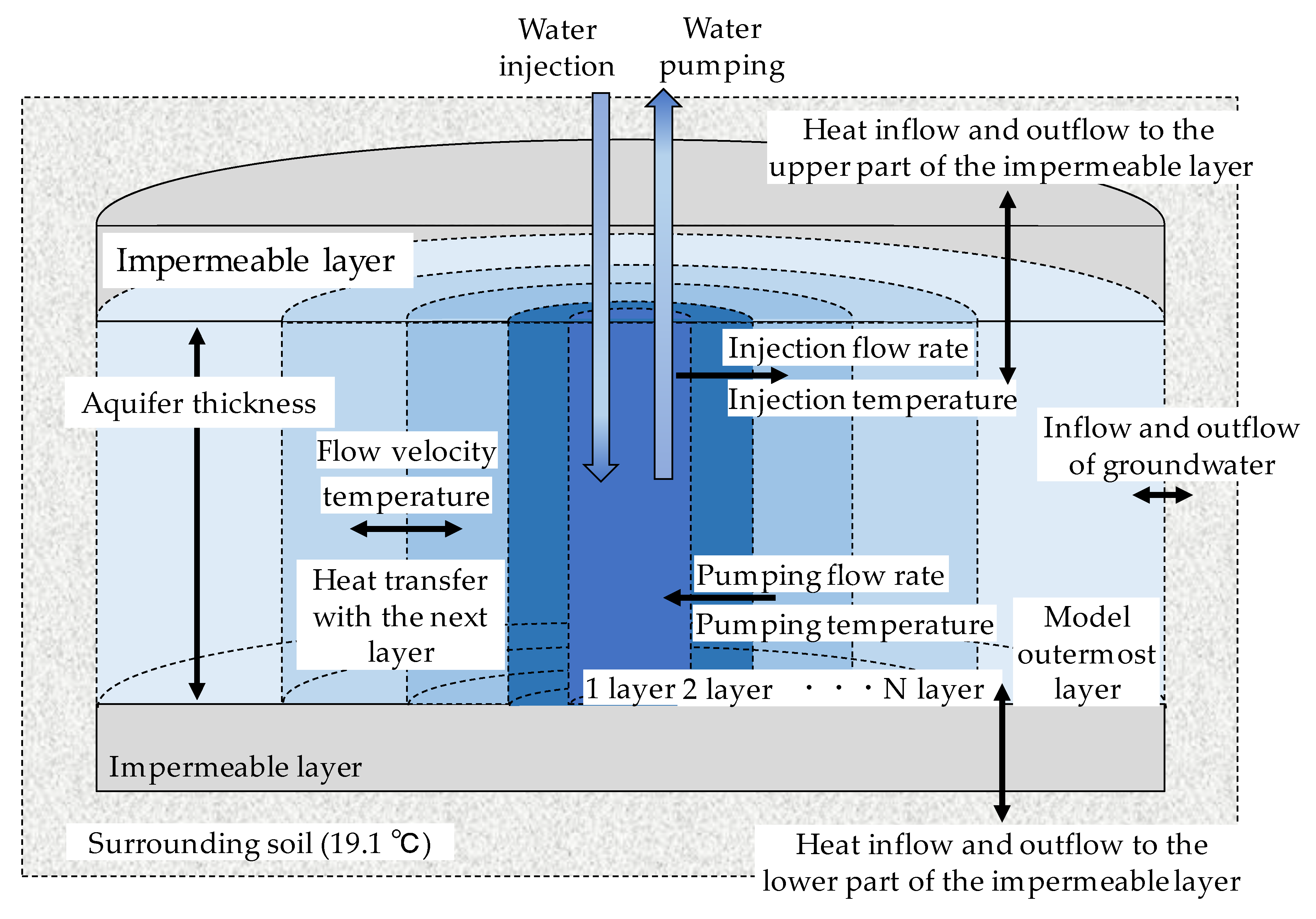
3.1. ATES Model

The aquifer model was created based on the cylindrical model of Nakaso et al. [29] and the energy equation in FEFLOW [30]. Figure 5 shows a conceptual diagram of the cylindrical model. In this model, multiple layers are set concentrically in a cylinder, assuming that the upper and lower parts are horizontal aquifers under pressure and sandwiched between impermeable layers. The groundwater flow velocity between layers is set to 0 m/s, and the heat transfer due to groundwater transfer is calculated. The water temperature and soil temperature in the same layer should be in equilibrium. Then, consider the heat loss due to heat conduction include the inner and outer layers. The outer edge (boundary) of the cylinder of the aquifer is opened and flows out from the outer edge by water injection to lose heat. In the pumping operation, groundwater at underground temperature flows in from the outer edge. For the cylindrical model, the condition values in Table 1 are used as model input values.
The parameter of the model was examined using the measured values in summer. In this model calculation formula, Appendix C shows the calculation formula of the thermophysical property value, and Appendix D shows the basic formula of the heat balance. The parameters of the model are calculated and given using these formulas. In this model, the effective thermal conductivity of the aquifer changes depending on the approximate dispersion length. Dispersion length is the degree to which the flow rate of a moving substance varies in a place where the flow rate is present. Furthermore, the thermal resistance of the aquifer is calculated from the thickness of the aquifer and the thickness of the impermeable layer. This parameter is identified using the condition of the target aquifer and the measured values to construct an aquifer model. However, the target aquifer (Figure 3) is not clearly separated by an impermeable layer above. It was difficult to reproduce the actual system only by adjusting the parameters of the approximate variance length. Therefore, we tried to reproduce the impermeable thickness by using the measured values of the impermeable layer thickness above and below the model in addition to the approximate dispersion length. Figure 6 shows the calculation results of the aquifer model and the actual temperature response comparison in the aquifer. The actual temperature response of the aquifer represents a temperature at a depth of 26 m. Table 2 shows the accuracy verification results using the root mean squared error (RMSE) of the results obtained by changing the approximate dispersion length and the permeable layer thickness. The parameters of the aquifer model were examined by changing the approximate dispersion length from 0.05 m to 0.4 m and the impermeable layer thickness from 0.002 m to 4 m. As a result of examining the parameters, the approximate dispersion length was 0.05 m and the impermeable layer thickness was 0.002 m. The impermeable layer thickness is a numerical value that represents the heat insulation performance of the aquifer, and the smaller it is, the more heat flows in and out from the surroundings. In reality, it is unlikely that such a thin impermeable layer exists, but this value was taken to reproduce the target aquifer without a clear impermeable layer.

3.2. Heat Source Model

The heat source model is constructed using the performance characteristics of the heat pump provided by the manufacturer (Figure 7). Table 3 shows the input and output data of the heat source model. The input values of the heat source model are the outside air temperature, the cooling water temperature, the outlet set temperature and the secondary load. The data collected by Building and Energy Management System (BEMS) are used for the outside air temperature and cooling water temperature. Figure 8 shows the cooling load and heating load and the outside air temperature of the building. The building load is calculated by Equation (1) using the cold/hot water inlet/outlet temperature and flow rate on the secondary side of the BEMS data. In the calculation of the heat source model, the maximum capacity is calculated from the performance characteristics of the heat source device provided by the manufacturer based on the outside air temperature, the cooling water inlet temperature and the chilled water outlet set temperature. We calculated the load factor by Equation (2). Power consumption is calculated by reading the coefficient of performance (COP) according to the load factor from the performance characteristics using the load factor of Equation (2) and the set temperature of the water cooling outlet. The amount of the processing heat of the heat pumps is the required amount of heat assuming the outlet set temperature. However, if the amount of heat-processed exceeds the maximum capacity, the outlet temperature is calculated assuming that the maximum capacity heat has been processed. The power consumption was calculated using the performance characteristics, but there was a large discrepancy with the power consumption of the measured data. Therefore, the calculated value is brought closer to the measured value by correcting the power consumption shown in Equations (3) and (4). The power consumption correction coefficient is identified monthly so that the corrected power consumption matches the measured value. The correction coefficient represents the difference between the calculated result and the measured value. The larger the correction coefficient is, the larger the measured power consumption is than the performance characteristic power consumption.
Q H e a t   L o a d = m × ρ × c p × ( t i n t o u t )
where Q H e a t   L o a d is the processing load [W], m is the flow rate of cold/hot water [m3/s], c p is the volumetric specific heat of water [J/(m3·K)], t i n is the water supply temperature [K], t o u t is the return water temperature [K].
η M a c h i n e = Q M a c h i n e Q R m a x
where η M a c h i n e is the load factor of heat pump [–], Q M a c h i n e is the amount of the processing heat of the heat pump [W], Q R m a x is maximum capacity of heat pump [W].
C F = W c a l c u l a t e d W m e a s u r e d
where C F is the power consumption correction coefficient of heat pump [–], W c a l c u l a t e d is the calculated result of power consumption [W], W m e a s u r e d is power consumption of heat pump measured value [W].
W C F = C F × W C
where W C F is corrected power consumption [W], C F is power consumption correction coefficient of heat pump [–] and W C is power consumption of heat pump according to performance characteristics [W].
The accuracy of the heat source model was verified using the measured values from 4 July to 6 2016. Figure 9 shows the accuracy verification results. In the figure, one point represents one hour. The heat source model calculates the COP using the power correction coefficient in Equation (2). The RMSE before power correction was 1.37, and after power correction, it was 0.62, which was improved by power correction.

4. Calculation Methods

4.1. Air Conditioning System Operating Method

Using the constructed model, we will examine the operation method of the ATES system according to the DR operation. Figure 10 shows the system diagram of the air conditioning system of the ATES system. The ATES system uses AHU precooling coil or preheating coil. Figure 11 shows the configuration of the AHU. In the ATES system, the heat pumps process the load at the same time when the building load processing capacity from the heat storage tank is insufficient. The night heat storage operation is from 22:00 to 8:00 (10 h), and the heat dissipation operation is from 8:00 to 18:00 (10 h). From 18: 00 to 22:00 (2 h), the operation of the heat pump stops. The heat pumps operate the cold water or hot water outlet temperature at 7 °C for cooling and 45 °C for heating. Three heat pumps are used. One heat pump performs heat storage operation through a heat exchanger 1 in the heat storage well at nighttime. In the daytime, the water pumped up from the heat storage well is sent to the AHU in the room through heat exchanger 2 for heat dissipation operation. After that, water is returned to the reduction well. Two heat pumps handle building loads at the same time with heat radiation operation of the ATES system.

4.2. Operation Case of ATES System Using DR

Table 4 shows the case settings. In case 0, the DR operation and the night heat storage operation are not performed. This is a case where the building load is processed only by the heat pumps. In Case 1-1 to Case 1-3, DR operation is predicted, and on days when DR operation does not occur, night heat storage operation is performed according to the case conditions. The nighttime heat storage operation time is 10 h, 6 h and 3 h in 3 cases. In case 2, the nighttime heat storage operation is stopped, and the DR operation is performed according to the prediction. In the DR heat storage operation, the DR heat storage operation is performed using a stopped heat pump. Each case has a run-up period of one month and is calculated for August. The calculation is performed continuously, and the calculation result of the previous time affects the next calculation. The water injection temperature is set to 7 °C and the groundwater temperature is set to 19.1 °C. The heat recovery rate of the aquifer model is assumed to be 82%. Nighttime heat storage operation is assumed to be able to handle 50% of the day with the highest load. For the input data, the building heat load, the outside air temperature, the cold water or hot water outlet set temperature, the cold water or hot water inlet temperature and the cooling water inlet temperatures are input.

5. Results and Discussion

Figure 12 shows a comparison of operation transitions on the representative days of each case. Case 0 uses heat pumps to handle the daily building load. On the other hand, in Case 1-1 to Case 1-3, which were operated in anticipation of DR occurrence, the nighttime heat storage operation on the day when DR occurred was stopped. According to DR, DR heat storage operation and heat dissipation operation are performed at the same time. The temperature at the time when the heat dissipation operation stopped is close to the groundwater temperature. It is an operation in which all the stored heat is used up. On days when DR does not occur, the heat storage operation time is adjusted according to the conditions of the case. Case 1-3, which had a nighttime heat storage operation time of 3 h, used up the amount of heat storage at 12 o’clock, and after 12 o’clock, the building load is processed by the water-cooled HP. Case 2, which was operated only by DR operation, mainly uses water-cooled HP to handle the building load on days when DR does not occur. In the case of using the aquifer heat storage system, the temperature of the water pumped from the heat storage well rises at 13:00. During this time, the temperature is returned to the reduction well at 20 °C or higher, and the heat of the groundwater originally in the aquifer is also used.
Figure 13 shows the amount of heat-processed and the amount of power consumed. Figure 13 summarizes the weekly data on which DR occurred continuously in August. In the case where the heat storage operation is performed, the amount of heat-processed by the heat dissipation operation is large. The smaller the amount of heat stored, the larger the amount of heat-processed by the water-cooled HP. The total power consumption is the same for Case 0, Case 1-3 and Case 2. In the operation that predicts DR, the shorter the nighttime heat storage operation time, the smaller the power consumption. In Case 2 where only DR operation is performed, the water-cooled HP handles the building load, so the power consumption of the water-cooled HP is the second largest after Case 0.
Figure 14 shows the ratio of heat-processed by water-cooled HP during the day and the rate of increase in power consumption. Figure 14 summarizes the weekly data on which DR occurred continuously in August. Each case is represented by day and is calculated by comparing with Case 0 of each day. The lower the processing heat amount ratio of the water-cooled HP, the more the building load is due to the heat dissipation operation is processed, and the daytime power consumption can be reduced. In Case 0, the water-cooled HP is used to handle the building load during the day. Therefore, the processing heat ratio of water-cooled HP is 100%. In Case 1-1 to Case 1-3, the processing heat ratio of water-cooled HP is lower than that of Case 0. Case 1-1 is about 30%, Case 1-2 is about 40% and Case 1-3 is about 70%. In this operation, the nighttime heat storage operation is performed on days when DR does not occur, so that the daytime power consumption is suppressed, but the total power consumption is increased by about 3% to 25%. On the other hand, in the case where the DR operation is predicted and the DR operation is performed, the processing heat amount ratio of the water-cooled HP is about 40% lower than that in the case 0 without increasing the total power consumption. The building load in the daytime is processed by the DR storage and heat dissipation operation while suppressing the power consumption in the daytime by the DR operation. Furthermore, in Case 1-1 and Case 1-2, which perform night heat storage operation for 6 h or more, we are able to utilize the excess heat of the previous day on the next day, and an energy-saving effect of about −3% was obtained. For this reason, in the operation of performing the night heat storage operation, the operation of using up as much as possible of the stored heat before DR occurs leads to the energy-saving operation.

6. Conclusions

In this study, we investigated an operation method that combines the surplus energy of photovoltaic power generation with an aquifer heat storage system using demand response (DR) that recognizes the power demand balance. The findings obtained in this study are shown below.
In the case, which predicts the occurrence of DR and performs DR storage and heat dissipation operation using the surplus energy of photovoltaic power generation, it has become an operation in which the total power consumption does not increase compared to Case 0 and the daytime power consumption can be suppressed.
Case 1-2, which performs nighttime heat storage operation for about 6 h, has become an operation that suppresses daytime power consumption by more than 60%. Furthermore, the increase in total power consumption was suppressed by combining DR heat storage operation.
By combining the nighttime heat storage operation and the DR operation, the stored heat could be used the next day and the total power consumption could be further reduced while suppressing the daytime power consumption.
In the case of night heat storage operation for a long time, the amount of heat storage was not used up. Therefore, it is better to operate to use up the heat stored at night as much as possible before DR occurs.
Even if the temperature of the water pumped from the heat storage well rises, the heat of the groundwater originally in the aquifer can be used in the preheating operation. However, since the underground temperature of the target area is 19.1 °C and the room temperature during cooling is about 25 °C, the heat of groundwater can be utilized.
The aquifer heat storage system in this study uses heat storage wells and reduction wells, and care must be taken in such an operation method depending on the layer configuration.
We have clarified the operation method of the ATES system that combines the nighttime heat storage operation and the DR heat storage operation. In the future, we will study how to operate an aquifer heat storage system that uses a large amount of surplus energy during the interim period throughout the year.

Author Contributions

All authors contributed to the study conception and design; writing—original draft preparation, J.O.; writing—review and editing, J.O., H.K. and D.S.; supervision, D.S.; project administration, D.S.; methodology, M.N.; formal analysis, M.N.; All authors have read and agreed to the published version of the manuscript.

Funding

This research received no external funding.

Institutional Review Board Statement

Not applicable.

Informed Consent Statement

Not applicable.

Data Availability Statement

Not applicable.

Acknowledgments

We would like to thank Shikoku Electric Power Co., Inc. and Yonden Consultants Co., Ltd. for their cooperation in advancing this research.

Conflicts of Interest

The authors declare no conflict of interest.

Appendix A

In aquifer heat storage, it is basic to reduce the pumped groundwater to the same aquifer as the pumped groundwater without contacting the air as much as possible. In the target building, when designing the aquifer heat storage system, we investigated the wells near the site and confirmed that the shallow well water (6 m well) was used as cold water by restaurants in the vicinity. Therefore, it was necessary to protect the cleanliness of the shallow well. The heat storage well (32 m well) and the reduction well (80 m well) contained a large amount of iron and manganese and were unsuitable for beverages. Therefore, after consulting with the relevant departments of the local government, it was judged that there would be no major problem with reduction. It is designed to store shallow well water in heat storage well and return it to a reduction well.

Appendix B

In the target building, the strainer of the reduction well is clogged and the overflow water that cannot be reduced is flowing into the sewer. Therefore, the aquifer heat storage system is not used daily. It is thought that the strainer can be cleaned by backwashing or chemicals, but this is not done due to consideration of groundwater pollution in the vicinity.

Appendix C

The formulas for calculating the thermophysical property values of the aquifer model are shown in Equations (A1)–(A6).
λ e s = ε · λ w + ( 1 ε ) · λ s
λ e c = ε · λ w + ( 1 ε ) · λ c
D i = α · u i · ( C p ) w
λ a , i = λ e s + D i
R a , i = 1 2 · λ a , i · π · H a · ln ( r i + 1 r i ) ( i = 1 , 2 , , n ) .  
R c , i = H c λ e c · S i ( i = 1 , 2 , , n )
where λ e _ s is synthetic thermal conductivity of the submerged layer [W/(m·K)], ε is gap ratio [–], λ w : is thermal conductivity of water [W/(m·K)], λ s is effective thermal conductivity of the gravel layer of the submerged layer [W/(m·K)], λ e _ c is synthetic thermal conductivity of the impermeable layer [W/(m·K)], λ c is clay Effective thermal conductivity [W/(m·K)], D i is thermal dispersion rate of the i layer [W/(m·K)], α is approximate dispersion length [m], u i is cross-section of the i layer Flow velocity [m/s], ( C p ) w is volumetric specific heat of the water [kJ/(m3·K)], λ a , i is thermal conductivity of the hydrous layer considering thermal dispersion [W/(m·K)], R a , i is the thermal resistance of the i layer [K/W], H a is aquifer thickness [m], r i is radius from the central axis [m], R c , i is thermal resistance from the i layer to an impermeable layer [K/W], H c is impermeable layer thickness [m], S i is layer bottom area [m2]

Appendix D

The equations for the heat balance of the aquifer model are shown in Equations (A7)–(A12).
  • Heat dissipation
Layer   1   ( c ρ ) e · V i · d θ i d t = ( c ρ ) w · m o u t ( θ i + 1 θ i ) + 1 R a , 1 ( θ i + 1 θ i ) + 1 R c , 1 ( θ s θ i )
Layer   i ~ N   ( c ρ ) e · V i · d θ i d t = ( c ρ ) w · m o u t ( θ i + 1 θ i ) + 1 R a , i 1 ( θ i 1 θ i ) + 1 R a , i ( θ i + 1 θ i ) + 1 R c , i ( θ s θ i )
  • Heat storage
Layer   1   ( c ρ ) e · V i · d θ i d t = ( c ρ ) w · m i n ( θ r θ i ) + 1 R a , 1 ( θ i + 1 θ i ) + 1 R c , 1 ( θ s θ i )
Layer   i ~ N   ( c ρ ) e · V i · d θ i d t = ( c ρ ) w · m i n ( θ i 1 θ i ) + 1 R a , i 1 ( θ i 1 θ i ) + 1 R a , i ( θ i + 1 θ i ) + 1 R c , i ( θ s θ i )
  • Stop
Layer   1   ( c ρ ) e · V 1 · d θ 1 d t = 1 R a , 1 ( θ 2 θ 1 ) + 1 R c , 1 ( θ s θ 1 )
Layer   i ~ N   ( c ρ ) e · V i · d θ i d t = 1 R a , i 1 ( θ i 1 θ i ) + 1 R a , i ( θ i + 1 θ i ) + 1 R c , i ( θ s θ i )
where ( c ρ ) e is the equivalent volume heat capacity of the gravel layer of the submerged layer [kJ/(m3·K)], V i is the volume of the i layer [m3], m i n is water injection flow [m3], m o u t is pumping water flow [m3], θ r is water injection temperature [K], θ i is the temperature of the i layer [K], θ s is ground Temperature [K], θ i + 1 is the temperature of the i+1 layer [K] and θ i 1 is the temperature of the i − 1 layer [K].

References

  1. Lund, H.; Mathiesen, B.V. Energy system analysis of 100% renewable energy system—The case of Denmark in years 2030 and 2050. Energy 2009, 34, 524–531. [Google Scholar] [CrossRef]
  2. Gyanwali, K.; Komiyama, R.; Fujii, Y. Representing hydropower in the dynamic power sector model and assessing clean energy deployment in the power generation mix of Nepal. Energy 2020, 202, 117795. [Google Scholar] [CrossRef]
  3. Lund, H. Large-scale integration of optimal combinations of PV, wind and wave power into the electricity supply. Renew. Energy 2006, 31, 503–515. [Google Scholar] [CrossRef]
  4. Albadi, M.H.; El-Saadany, E.F. A summary of demand response in electricity markets. Electr. Power Syst. Res. 2008, 78, 1989–1996. [Google Scholar] [CrossRef]
  5. Palensky, P.; Dietrich, D. Demand Side Management: Demand Response, Intelligent Energy Systems, and Smart Loads. IEEE Trans. Ind. Inform. 2011, 7, 381–388. [Google Scholar] [CrossRef] [Green Version]
  6. Janota, L.; Králík, T.; Knápek, J. Second Life Batteries Used in Energy Storage for Frequency Containment Reserve Service. Energies 2020, 13, 6396. [Google Scholar] [CrossRef]
  7. Kalantari, H.; Ghoreishi-Madiseh, S.A.; Sasmito, A.P. Hybrid Renewable Hydrogen Energy Solution for Application in Remote Mines. Energies 2020, 13, 6365. [Google Scholar] [CrossRef]
  8. Misaki, C.; Hara, D.; Katayama, N.; Dowaki, K. Improvement of Power Capacity of Electric-Assisted Bicycles Using Fuel Cells with Metal Hydride. Energies 2020, 13, 6272. [Google Scholar] [CrossRef]
  9. Bloemendal, M.; Olsthoorn, T.; Boons, F. How to achieve optimal and sustainable use of the subsurface for Aquifer Thermal Energy Storage. Energy Policy 2014, 66, 104–114. [Google Scholar] [CrossRef]
  10. Lee, K.S. A Review on Concepts, Applications, and Models of Aquifer Thermal Energy Storage Systems. Energies 2010, 3, 1320–1334. [Google Scholar] [CrossRef]
  11. Pinamonti, M.; Prada, A.; Baggio, P. Rule-Based Control Strategy to Increase Photovoltaic Self-Consumption of a Modulating Heat Pump Using Water Storages and Building Mass Activation. Energies 2020, 13, 6282. [Google Scholar] [CrossRef]
  12. Vanhoudt, D.; Desmedt, J.; Van Bael, J.; Robeyn, N.; Hoes, H. An aquifer thermal storage system in a Belgian hospital: Long-term experimental evaluation of energy and cost savings. Energy Build. 2011, 43, 3657–3665. [Google Scholar] [CrossRef]
  13. Paksoy, H.; Gürbüz, Z.; Turgut, B.; Dikici, D.; Evliya, H. Aquifer thermal storage (ATES) for air-conditioning of a supermarket in Turkey. Renew. Energy 2004, 29, 1991–1996. [Google Scholar] [CrossRef]
  14. Xu, J.; Wang, R.; Li, Y. A review of available technologies for seasonal thermal energy storage. Sol. Energy 2014, 103, 610–638. [Google Scholar] [CrossRef]
  15. Bloemendal, M.; Jaxa-Rozen, M.; Olsthoorn, T. Methods for planning of ATES systems. Appl. Energy 2018, 216, 534–557. [Google Scholar] [CrossRef]
  16. Bloemendal, M.; Hartog, N. Analysis of the impact of storage conditions on the thermal recovery efficiency of low-temperature ATES systems. Geothermics 2018, 71, 306–319. [Google Scholar] [CrossRef]
  17. Kranz, S.; Frick, S. Efficient cooling energy supply with aquifer thermal energy storages. Appl. Energy 2013, 109, 321–327. [Google Scholar] [CrossRef]
  18. Sommer, W.; Valstar, J.; Leusbrock, I.; Grotenhuis, T.; Rijnaarts, H. Optimization and spatial pattern of large-scale aquifer thermal energy storage. Appl. Energy 2015, 137, 322–337. [Google Scholar] [CrossRef]
  19. Bloemendal, M.; Olsthoorn, T.; van de Ven, F. Combining climatic and geo-hydrological preconditions as a method to determine world potential for aquifer thermal energy storage. Sci. Total Environ. 2015, 538, 621–633. [Google Scholar] [CrossRef] [PubMed] [Green Version]
  20. Wang, H.; Qi, C.; Wang, E.; Zhao, J. A case study of underground thermal storage in a solar-ground coupled heat pump system for residential buildings. Renew. Energy 2009, 34, 307–314. [Google Scholar] [CrossRef]
  21. Zhai, X.; Qu, M.; Yu, X.; Yang, Y.; Wang, R. A review for the applications and integrated approaches of ground-coupled heat pump systems. Renew. Sustain. Energy Rev. 2011, 15, 3133–3140. [Google Scholar] [CrossRef]
  22. Bozkaya, B.; Zeiler, W. The effectiveness of night ventilation for the thermal balance of an aquifer thermal energy storage. Appl. Therm. Eng. 2019, 146, 190–202. [Google Scholar] [CrossRef]
  23. Gao, L.; Zhao, J.; An, Q.; Wang, J.; Liu, X. A review on system performance studies of aquifer thermal energy storage. Energy Procedia 2017, 142, 3537–3545. [Google Scholar] [CrossRef]
  24. Caliskan, H.; Dincer, I.; Hepbasli, A. Energy and exergy analyses of combined thermochemical and sensible thermal energy storage systems for building heating applications. Energy Build. 2012, 48, 103–111. [Google Scholar] [CrossRef]
  25. Yang, W.; Zhou, J.; Xu, W.; Zhang, G. Current status of ground-source heat pumps in China. Energy Policy 2010, 38, 323–332. [Google Scholar] [CrossRef]
  26. Bozkaya, B.; Li, R.; Zeiler, W. A dynamic building and aquifer co-simulation method for thermal imbalance investigation. Appl. Therm. Eng. 2018, 144, 681–694. [Google Scholar] [CrossRef]
  27. Zhou, X.; Gao, Q.; Chen, X.; Yan, Y.; Spitler, J.D. Developmental status and challenges of GWHP and ATES in China. Renew. Sustain. Energy Rev. 2015, 42, 973–985. [Google Scholar] [CrossRef]
  28. Shikoku Electric Power Co., Inc. Electricity Forecast (Electricity Usage in Shikoku Area). Available online: https://www.yonden.co.jp/nw/denkiyoho/index.html (accessed on 4 December 2020).
  29. Nakaso, Y.; Sasaki, K.; Fujii, R.; Nakao, M.; Nishioka, M.; Nnabeshima, M. Study on Daily Thermal Storage System ufflizing High Closure Aquifer Part2—Experiment and Verification with ATES Model. Soc. Heat. Air-Cond. Sanit. Eng. Jpn. 2013, 38, 11–18. [Google Scholar] [CrossRef]
  30. FEFLOW Manual. Available online: http://www.feflow.infouploadsmediauser_manual.pdf (accessed on 4 December 2020).
Figure 1. The number of DR occurrences by month and time.
Energies 14 03129 g001
Figure 2. The DR occurrence change (One week in the interim period as the representative days).
Energies 14 03129 g002
Figure 3. The stratum diagram of the heat storage well.
Energies 14 03129 g003
Figure 4. The experimental data of the ATES system: (a) The temperature response inside the heat reservoir well; (b) The water injection and pumps flow rate in the heat reservoir.
Energies 14 03129 g004
Figure 5. A conceptual diagram of the cylindrical model.
Energies 14 03129 g005
Figure 6. The calculation results of the aquifer model and the actual temperature response comparison in the aquifer: dispersion length of (a) dispersion length 0.002 m; (b) dispersion length 4 m.
Energies 14 03129 g006
Figure 7. The performance characteristics of the heat pump: (a) Cooling performance characteristics; (b) Heating performance characteristics.
Energies 14 03129 g007
Figure 8. The cooling load and heating load and the outside air temperature of the building.
Energies 14 03129 g008
Figure 9. Accuracy verification results of heat pumps.
Energies 14 03129 g009
Figure 10. System diagram of air conditioning system for ATES system.
Energies 14 03129 g010
Figure 11. System diagram of AHU for ATES system.
Energies 14 03129 g011
Figure 12. A comparison of operation transitions on the representative days of each case: (a) Water-cooled HP operation; (b) 10-h nighttime heat storage operation and DR heat storage operation; (c) 3-h night heat storage operation and DR heat storage operation; (d) DR heat storage operation.
Energies 14 03129 g012
Figure 13. Processing heat and power consumption.
Energies 14 03129 g013
Figure 14. Water-cooled HP processing heat load ratio and rate of increase in power consumption.
Energies 14 03129 g014
Table 1. The cylindrical model input values.
Radius [m]20
Initial division width [m]0.03
common ratio [–]1.10
AquiferVolumetric specific heat [MJ/(m3·K)]3.18
Effective thermal conductivity [W/(mK)]1.6
Clearance rate [–]0.3
clayVolumetric specific heat [MJ/(m3·K)]3.06
Effective thermal conductivity [W/(m·K)]1.2
Clearance rate [–]0.3
WaterVolumetric specific heat [MJ/(m3·K)]4.18
Thermal conductivity [W/(m·K)]0.59
Aquifer thickness [m]8
Dispersion length [m]Change
Impermeable layer thickness [m]Change
Initial underground temperature [°C]19.1
Table 2. The accuracy verification results using the root mean squared error (RMSE) of the results obtained by changing the approximate dispersion length and the permeable layer thickness.
Thickness of Impervious LayerDispersion Length
0.05 m
Dispersion Length
0.1 m
Dispersion Length
0.2 m
Dispersion Length
0.3 m
Dispersion Length
0.4 m
0.002 m0.781.031.071.491.83
0.005 m0.871.161.061.451.75
0.1 m0.951.261.061.431.76
4 m0.951.271.061.431.76
Table 3. The input and output data of the heat source model.
Input DataOutput Data
  • Processing load
  • Cold/hot water outlet set temperature
  • Cold/hot water inlet temperature
  • Outside air temperature
  • Cooling water temperature
  • Cooling water flow rate
  • Cold/Hot water outlet temperature
  • Processing capacity
  • Power consumption
  • COP
Table 4. Case setting using the DR operation.
CaseCase Contents
Case 0Water-cooled HP operation
No heat storage operation
Case 1-1Night heat storage 10 h, DR operation
Case 1-2Night heat storage 6 h, DR operation
Case 1-3Night heat storage 3 h, DR operation
Case 2DR operation
  • Aquifer heat recovery rate: 82%
  • Calculation period: 1 month as run-up period, August
  • Water injection temperature: 7 °C
  • Groundwater temperature: 19.1 °C
  • Input data are building heat load, outside air temperature, cold/hot water outlet set temperature, cold/hot water inlet temperature, cooling water inlet temperature
Publisher’s Note: MDPI stays neutral with regard to jurisdictional claims in published maps and institutional affiliations.

