Effect of Symmetrically Switched Rectifier Topologies on the Frequency Regulation of Standalone Micro-Hydro Power Plants

Abstract

Micro-hydro power plants (μHPPs) are a major energy source in grid-isolated zones because they do not require reservoirs and dams to be built. μHPPs operate in a standalone mode, but a continuously varying load generates voltage unbalances and frequency fluctuations which can cause long-term damage to plant components. One method of frequency regulation is the use of alternating current-alternating current (AC-AC) converters as an electronic load controller (ELC). The disadvantage of AC-AC converters is reactive power consumption with the associated decrease in both the power factor and the capacity of the alternator to deliver current. To avoid this disadvantage, we proposed two rectifier topologies combined with symmetrical switching. However, the performance of the frequency regulation loop with each topology remains unknown. Therefore, the objective of this work was to evaluate the performance of the frequency regulation loop when each topology, with a symmetrical switching form, was inserted. A MATLAB^® model was implemented to simulate the frequency loop. The results from a μHPP case study in a small Cuban rural community called ‘Los Gallegos’ showed that the performance of the frequency regulation loop using the proposed topologies satisfied the standard frequency regulation and increased both the power factor and current delivery capabilities of the alternator.

1. Introduction

Over 170 small-scale hydro power plants (HPPs) supply 1% of electrical power in Cuba, mainly in the Oriental Province of the island which operates as an autonomous system, isolated from the main electrical grid. According to the International Hydropower Association, the Cuban government has aspirations to significantly increase its share of renewables over the next two decades, aiming to generate some 24% of the country’s electricity by 2030. With no major rivers or large bodies of inland water, Cuba’s development of hydropower will remain focused on small projects. The technical potential of small hydro power is estimated at 135 MW. Thus, the government has drawn up plans to develop 74 HPPs with a capacity of over 56 MW (274 GWh). This would nearly double the country’s current hydropower capacity, generating an estimated 274 GWh of renewable energy annually and offsetting up to 230,000 tonnes of CO₂ emissions [1].

In this context, the micro hydro power plants (μHPPs) play a very important role. There are hydro power plants delivering power from 5 kW up to 100 kW [2,3,4]. In Cuba, 117 μHPPs support the electrification of off-grid rural areas and operate in autonomous regimens [5]. This means that each μHPP having only one alternator must supply energy to a small grid of consumer without electrical connection to another electrical source. For that reason, they are called standalone μHPP. These μHPPs are run-of-river plants such as described in [2,6] and they have the advantage that they do not require big volumetric water flows and produce less harmful environmental impact compared with diesel generators, for example.

For a standalone μHPP, it is very important to keep the balance between the power production by the alternator and the power consumption by the user at all time, because if this balance is not kept, the frequency fluctuates. Frequency fluctuations can cause mechanical vibrations, overheating, and long-term damage to electrical devices [7]. For that reason, in standalone μHPPs is obligatory to implement some technique to regulate frequency. There are two ways to accomplish it using either control flow by employing mechanical hydraulic governors or by using electrical control [8].

Mechanical hydraulic governors are not usually considered in these projects because they have a slower dynamic response, high maintenance, high economic cost and due to the water hammer phenomena when the water flow in the turbine needs to be reduced abruptly. Therefore, alternative methods of electrical frequency regulation must be implemented in order to achieve high reliability at these plants [8,9].

Most of these methods use power electronics converters [10,11] but these introduce harmonics and increase switching losses in the system. To reduce the losses, some switching techniques are used such as soft switching techniques, zero voltage switching (ZVS) or zero current switching (ZCS). In [12], the authors propose the use of a ZVS–PWM active clamp/reset forward converter to reduce switching power losses with the use of a constant frequency and PWM operation. In [13], the authors propose a control algorithm based on frequency bus-signaling of the energy storage system and uses only local measurements for power distribution among microgrid elements. There are other more complex algorithms such as that presented in [14], which is a meta-heuristic algorithm, namely ant lion optimizer (ALO), and was used to solve the load frequency control problem under load disturbances. The performance of ALO was evaluated using three case studies of multiarea power systems. However, these methods are usually used in large grids with multiple suppliers and consumers. In those cases, the control system of the energy system architecture requires a control hierarchy that includes primary, secondary and tertiary controls [15].

In standalone μHPPs, only primary control is needed and the most common method is the use of a dummy or ballast load to shed the excess energy that is not being consumed [8,16]. Thus, the active power supplied by the alternator (P_G) must equal the dissipated power by the ballast load (P_L) and the active power consumed by users (P_U): P_G = P_L + P_U. As shown in Figure 1 electronic controllers with resistive loads that can mediate this balance are known as electronic load controllers (ELCs).

The advantages of the ELC are the incorporation of simpler and cheaper turbine with less moving part in the micro-hydro architecture; the absence of hammer effect from load changes; less robust penstock and also less wear on the hydro power plant’s mechanical parts; it has high reliability, low maintenance and simple operation principle; it can be installed anywhere in the electrical system; and the ballast load can be used as a heater for water or households, resulting in 100% load factor of the μHPP [8,17,18].

The authors of the papers [8,18,19] agree that, for a micro-hydro system supplying rural load for which cost-effectiveness is the major factor, ELC is the best way of regulating the frequency. ELC can be made using different methods, systems or approaches. The selection of ELCs depends on the capacity of the power plant.

Existing types of ELC use three sets of dummy loads and three sets of power electronic switch for controlling the power of each phase. In [20], the authors present a method for controlling power consumed from each phase by using a single dummy load and a single power electronic switch, which reduces the component count and the associated costs. In [21], in order to regulate the μHPP frequency, an ELC control strategy with a self-tuning fuzzy PI controller is proposed in which the controller gains are adjusted in real-time using a fuzzy logic inference system. In [9], a similar design of fuzzy logic-based controller is presented.

In [22], a PWM-based alternating current–direct current–alternating current (AC-DC-AC) converter implemented for a three-phase self-excited induction generator (SEIG)-based micro hydro power generation is presented. In [23] two units of three phase capacitor-excited asynchronous generators (CAGs) operating in parallel are used. The μHPP utilizes PWM-based AC-DC-AC converter to provide constant frequency and voltage. In [24] the authors use thyristors to maintain a constant load at the generator using a dummy load controlled. The control unit checks the line frequency and, according to it, generates specific pulses of required firing angle. The pulses are then passed to control the gate of the thyristor to which the dummy load is connected. The proposed control unit is designed and then integrated between the generator and load to monitor the line frequency and compare it with the standard imposed by the energy market in Pakistan. According to the author, the cost of the proposed ELC is much lower as compared to those available in the market but the paper does not include the cost of the solution. A similar method is used in [16]. In this case, an ELC for synchronous generator of micro hydro power plant of rating 60 kW is used. The authors propose a controlled bridge rectifier and insulated-gate bipolar transistor (IGBT) chopper feeding a resistive dump load.

In [19], the design and implementation of an ELC is presented as an alternative to a speed governor required for regulating the frequency of supply under varying load conditions. This is the single most expensive component in a μHPP and most of the community owned plants in Africa can hardly afford it. Magnetostrictive amorphous wire (MAW) is used as a frequency sensor. They use a Proportional-Integral (PI) to control the frequency. According to the authors, the controller is able to respond in 1.5 s to stabilize the frequency between 49.5 and 50.5 Hz when there is a change in consumer load. The designed controller costs $229.25, which is cheaper when compared to other ELCs and speed governors that are currently on the market. In [17], a distributed electronic load controller (DELC) installed in each household is proposed instead of a single dump-load at the generating site. This decreases system vulnerability to component failures while also diverting surplus power into household heaters to pasteurize water or slow-cook food. This can be particularly suitable for Nepal’s mountainous terrain and remote communities.

Because of the high cost of other alternatives, AC-AC converters are used as the ELC to vary the power dissipated in dump loads in Cuba. The major disadvantage of AC-AC converters is their inherent reactive power consumption, which aggravates the power factor at the alternator output terminals and hence decreases its capacity to deliver current.

Therefore, three-phase and single-phase rectifier topologies combined with symmetrical switching were proposed as an alternative [5] because they are able to avoid reactive power consumption (Figure 2). For both rectifier topologies, R represents the dump load and IS is an IGBT. The cost of these topologies depends on the number and the cost of the main power devices.

Table 1. Cost of the topologies for ELC using the data of the Los Gallegos case of study.

Topology	Device	Quantity	Unit Price (€)	Total Cost (€) 1
AC-AC Converter	Thyristor SKT 55/04 D	6	25.65	153.90
	R 4 kW	3	9.65	28.95
	Total			182.85
Three-phase rectifier with symmetrical switching	Rectifier SQL40A	1	10.27	10,27
	IGBT SKM400GAL12	1	44.25	44.25
	R 12kW	1	11.50	11.50
	Total			66.02
Single phase rectifier with symmetrical switching	Rectifier FB5006	3	1.82	5.46
	IGBT SKM400GAL12	3	44.25	132.75
	R 4 kW	3	9.65	28.95
	Total			167.16

¹ For this cost, the monetary change by the BCC on 31 October, 2020 was use (1 € = 1.13 USD).

shows a comparative of the cost of the three topologies.

In Figure 3 the line current waveforms for the AC-AC converter are plotted, ILACAC, and the single-phase rectifier switched with symmetrical switching, ILBD1, to show the differences in the current line due to different switching form. However, the effect of the proposed rectifiers and symmetrical switching control on the frequency regulation loop performance and improvement of the power factor have not yet been analyzed in the literature.

Thus, the main goal of this present paper was to evaluate the frequency regulation loop and power factor performance of a μHPP when a three-phase rectifier and single-phase rectifier, both with symmetrical switching, were used for frequency regulation. In Section 2, we present the functional diagram of the μHPP and describe the mathematical model of the μHPP components. In addition, we also demonstrate the mathematical models in deviation variable of the alternator mechanical part and the proposed rectifier topologies. In Section 3, we present the scheme (implemented in MATLAB/Simulink^®) we propose using it to simulate the frequency regulation loop and to obtain some variables such as the root mean square (RMS) current, power factor, and active, reactive, and apparent power. In Section 4, we evaluate the performance of the frequency regulation loop when the proposed topologies used as the ELC were employed. In addition, we compared these topologies with the AC-AC ELC converter currently used in Cuban μHPPs. Finally, our conclusions are presented in Section 5.

2. Modeling the Frequency Regulation Loop

The functional diagram of frequency regulation using ELC for a standalone μHPP is shown in Figure 4.

2.1. Hydraulic Turbine

The motive power developed by the turbine (Pm) is given by [2,18,25]:

$$P_m={\eta }_t\rho g{Q}_V{H}_n,$$

(1)

where η_t is the turbine efficiency, which is dimensionless, ρ is the water density in kg/m³, g is the acceleration due to gravity in m/s², Q_V is the water flow rate in m³/s, and H_n is the net head in m.

2.2. Alternator Mechanical Part

Some articles employ a model of the alternator mechanical part that considers the damping produced by the alternator bar damper when the rotor speed is different to the synchronous speed [26,27]. However, this is incorrect for alternators that operate without a connection with other voltage sources, as is the case of standalone μHPPs.

Newton’s law applied to the turbine alternator system is:

$$J_T\frac{d}{dt}{w}_{rm}=T_M-T_G-T_{F,}$$

(2)

where J_T is the total inertia of the turbine alternator in kg m², T_M is the turbine motive torque on the alternator shaft in N⋅m, T_G is the alternator electrical torque in N⋅m, T_F is the total torque due to turbine and alternator windage friction exerted upon the alternator shaft in N⋅m, and w_rm is the alternator rotor speed in mechanical rad/s.

The magnitude T_F is defined as: T_F = K_F⋅w_rm, where K_F is the friction coefficient in N⋅m⋅s/rad.

Multiplying (2) by w_rm we obtain:

$$J_T{w}_{rm}\frac{d}{dt}{w}_{rm}=P_M-P_G-K_F{w}_{rm}^2,$$

(3)

where the P_M turbine motive power is in W and the P_G electrical power is delivered by the alternator in W.

Equation (3) is non-linear and so, as the alternator operates at speeds near the mechanical synchronous speed, w_rmo, the following deviation variables around the operation point (OP) are defined:

$$\begin{array}{c}{w}_{rm}=w_{rmo}+\Delta w_{rm}\\ P_M=P_{Mo}+\Delta P_M\\ P_G=P_{Go}+\Delta P_G\end{array},$$

(4)

where the subscript o indicates values corresponding to the OP.

By substituting (4) in (3), recognizing that at the OP

$$0=P_{Mo}-P_{Go}-K_F{w}_{rmo}^2,$$

and ignoring second-order terms, the following expression is obtained:

$$J_T{w}_{rmo}\frac{d}{dt}\Delta w_{rm}+2K_F{w}_{rmo}\Delta w_{rm}\approx \Delta P_M-\Delta P_G$$

(5)

As ΔP_G = ΔP_U + ΔP_L, where ΔP_U and ΔP_L are the incremental user power consumption and power dissipated by the dump load around the OP, respectively. Moreover, recognizing that:

$$w_{rm}=\raisebox{1ex}{$4\pi f$}\!\left/ \!\raisebox{-1ex}{$P$}\right. \mathrm{and} w_{rmo}=\raisebox{1ex}{$4\pi f_o$}\!\left/ \!\raisebox{-1ex}{$P$}\right.,$$

where P is the alternator number of poles, f is the electrical frequency, and f_o = 60 Hz, (5) is transformed into:

$$J_T{\left(\frac{4\pi }{P}\right)}^2{f}_o\frac{d}{dt}\Delta f+2{\left(\frac{4\pi }{P}\right)}^2{f}_o{K}_F\Delta f=\Delta P_M-\Delta P_U-\Delta P_L$$

(6)

Laplace transformation is used to obtain the transfer function (TF) of (6), thereby obtaining:

$$\Delta F\left(s\right)=\frac{\frac{P^2}{2{\left(4\pi \right)}^2{f}_o{K}_F}}{\frac{J_T}{2K_F}s+1}\left[\Delta P_M\left(s\right)-\Delta P_U\left(s\right)-\Delta P_L\left(s\right)\right]$$

(7)

Now, the two constants can be defined as follows:

K_G = P²/{2(4π)²f_oK_F} for the alternator gain in Hz/W and T_G = J_T/(2K_F) as the mechanical time constant in s.

2.3. User Load

The load models are classified into two broad categories, static models and dynamic models [28]. In this work, a physical model block implemented in MATLAB/Simulink^® was used to simulate the different user or consumer conditions.

2.4. Mathematical Model of the Converter Topologies Being Studied

In this topic the modelling method used in [29] is applied to obtain the TF for the different converters.

The mathematical expression that relates the power at the input of the rectifier (P_L) with the voltage (M) that the regulator sends to the control unit (CU) is:

$$P_L\left(t\right)=K_C·u\left(t-T_C\right)M\left(t\right),$$

(8)

where Tc is the mean value of the time delay from when the M signal change until the input power of the rectifier responds, and u( ) is the step function. The parameter Kc is determined as Kc = Pmax/Mmax, which will be demonstrated later. It represents the gain of the converter where Pmax is the maximum power consumed by the converter and Mmax is the maximum value of the CU input. Notice that for rectifier of Figure 2b, P_L, is the total power, because there is one rectifier for each phase.

Because Equation (7) relates the incremental power dissipated by the dump load, ΔP_L, with the incremental frequency, ΔF, around the OP, it is necessary to transform Equation (8) using the deviation variable. Around the OP:

$$P_L\left(t\right)=P_{Lo}+\Delta P_L \mathrm{and} M\left(t\right)=M_o+\Delta M$$

(9)

where P_Lo y M_o are respectively the power dissipated by the dump load and the signal sent by the controller to the CU of the converter, at the OP.

By substituting (9) in (8) and recognizing that at the OP,

$$P_{Lo}=K_C·u\left(t-T_C\right)M_o$$

The following expression is obtained:

$$\Delta P_L\left(t\right)=K_C·u\left(t-T_C\right)\Delta M\left(t\right),$$

(10)

Thus, applying the Laplace transformation to (10), the following expression is obtained:

$$\Delta P_L\left(s\right)=K_C{e}^{-T_{C}s}\Delta M\left(s\right)$$

(11)

Then, using the Pade approximation, the TF is given by:

$$\Delta P_L\left(s\right)=\frac{K_C}{T_{C}s+1}\Delta M\left(s\right)$$

(12)

Thus, for three-phase systems, Tc is approximately equal to 0.001 s [29]. Applying the same logic, the TF for the set of three single-phase AC-AC converters, one for each phase, is given by (12). This equation has the same structure given in [30].

Now it will be demonstrated that Kc = Pmax/Mmax.

The parameter Kc relates the change in the power consumed by the converter or dissipated by the dump load, P_L, with the change of the signal M applied to the CU. As P_L is function of the switching angle α [5] and, at the same time, α is function of M, this parameter is given as:

$$K_C=\frac{d{P}_L}{d\alpha }·\frac{d\alpha }{dM}$$

(13)

For the AC-AC converters, the variation range for α is from 0 to π, so the CU has the following lineal relation:

$$\alpha =\pi -\frac{M}{M_{max}}·\pi$$

(14)

Note that, when the signal M is zero, the firing angle is equal to π and for Mmax, α is zero.

Taking the derivative of (14) with respect to M,

$$\frac{d\alpha }{dM}=-\frac{\pi }{M_{max}}$$

(15)

which is a constant value.

For the set of three AC-AC converters, the expression of P_L, given in [5], is:

$$P_L=P_{max}\left\{\pi -\alpha +\frac{\sin \left(2\alpha \right)}{2}\right\}$$

(16)

By taking the derivative of P_L respect to α, the next equation is obtained

$$\frac{d{P}_L}{d\alpha }=-\frac{P_{max}}{\pi }+\frac{P_{max}}{\pi }cos\left(2\alpha \right)$$

(17)

Multiplying (15) by (17), the parameter Kc is obtained as:

$$K_C\left(\alpha \right)=\frac{P_{max}}{\pi }\left\{1+cos\left(2\alpha \right)\right\}$$

(18)

Equation (18) shows that the parameter Kc depends of the α value. To eliminate this dependence, the mean value of Kc for different values of α is taken. This corresponds to linearizing the curve Kc around different values of α. Proceeding in this way for the α values π/6, π/2 and 5π/6, the following expression is obtained:

$$K_C=\frac{\frac{P_{max}}{2M_{max}}+\frac{2P_{max}}{M_{max}}+\frac{P_{max}}{2M_{max}}}{3}=\frac{P_{max}}{M_{max}}$$

(19)

A similar logic is applied to get Kc for the set of three single-phase rectifiers with symmetrical switching.

It is known from [5] that α is within the interval 0 ≤ α ≤ π/2, hence its CU relates α with M by the following equation:

$$\alpha =\frac{\pi }{2}-\frac{M}{M_{max}}·\frac{\pi }{2}$$

(20)

Note that, when the signal M is zero, the switching angle is equal to π/2 and when is Mmax, α is zero.

By taking the derivative of (20) with respect to M, the following relationship is obtained:

$$\frac{d\alpha }{dM}=-\frac{\pi }{2M_{max}}$$

(21)

which is a constant value.

For the set of three single-phase rectifiers, P_L is [5]:

$$P_L=\frac{P_{max}}{\pi }\left\{\pi -2\alpha +\sin \left(2\alpha \right)\right\}$$

(22)

By taking the derivative of (22) with respect to α, the next equation is obtained

$$\frac{d{P}_L}{d\alpha }=-\frac{2P_{max}}{\pi }+\frac{2P_{max}}{\pi }cos\left(2\alpha \right)$$

(23)

To determine the parameter Kc, the expressions (21) and (23) are multiplied, resulting

$$K_C\left(\alpha \right)=\frac{P_{max}}{\pi }\left\{1+cos\left(2\alpha \right)\right\}$$

(24)

As in the case of the AC-AC converters, the parameter Kc depends on α value. To eliminate this dependence, the mean value of Kc for the following values of α, π/6, π/4 and π/3 is taken, obtaining:

$$K_C=\frac{\frac{P_{max}}{2M_{max}}+\frac{P_{max}}{M_{max}}+\frac{3P_{max}}{2M_{max}}}{3}=\frac{P_{max}}{M_{max}}$$

(25)

In the case of the three-phase rectifiers with symmetrical switching, a simpler expression is obtained because P_L vs. α is almost linear:

$$\raisebox{1ex}{$d{P}_L$}\!\left/ \!\raisebox{-1ex}{$d\alpha $}\right.\approx -\raisebox{1ex}{$P_{max}$}\!\left/ \!\raisebox{-1ex}{$M_{max}$}\right.$$

Moreover, it is known from [5] that α is within the interval 0 ≤ α ≤ π/6, hence its CU is modeled by:

$$\alpha =\frac{\pi }{6}-\frac{M}{M_{max}}·\frac{\pi }{6}$$

(26)

Note that, when the signal M is zero, the switching angle is equal to π/2 and when M is Mmax, α is zero.

The result of taking the derivative of (26) with respect to M, gives a constant value.

$$\frac{d\alpha }{dM}=-\frac{\pi }{6M_{max}}$$

(27)

Then the parameter Kc is constant as shown by (28)

$$K_C=\frac{P_{max}}{M_{max}}$$

(28)

Notice that the converters analyzed have the same equation of Kc given by (19), (25) and (28). Therefore, different ELCs have the same TF without considering the topology of converters and switching form. Another advantage is that for a specific application, the set of parameters of the frequency regulator are not depending of the type of converter used as ELC.

The value Kc is needed only for computing the frequency regulator parameter, because each topology will be implemented using physical model blocks of MATLAB/Simulink^® shown in the next section.

3. Scheme Implemented in MATLAB/Simulink^®

Figure 5 shows the model implemented in MATLAB/Simulink^® to evaluate the effect of the different topologies on the performance of the frequency regulation loop. Moreover, its components can be configured to suit any μHPP.

The main blocks of the model shown in Figure 5 are:

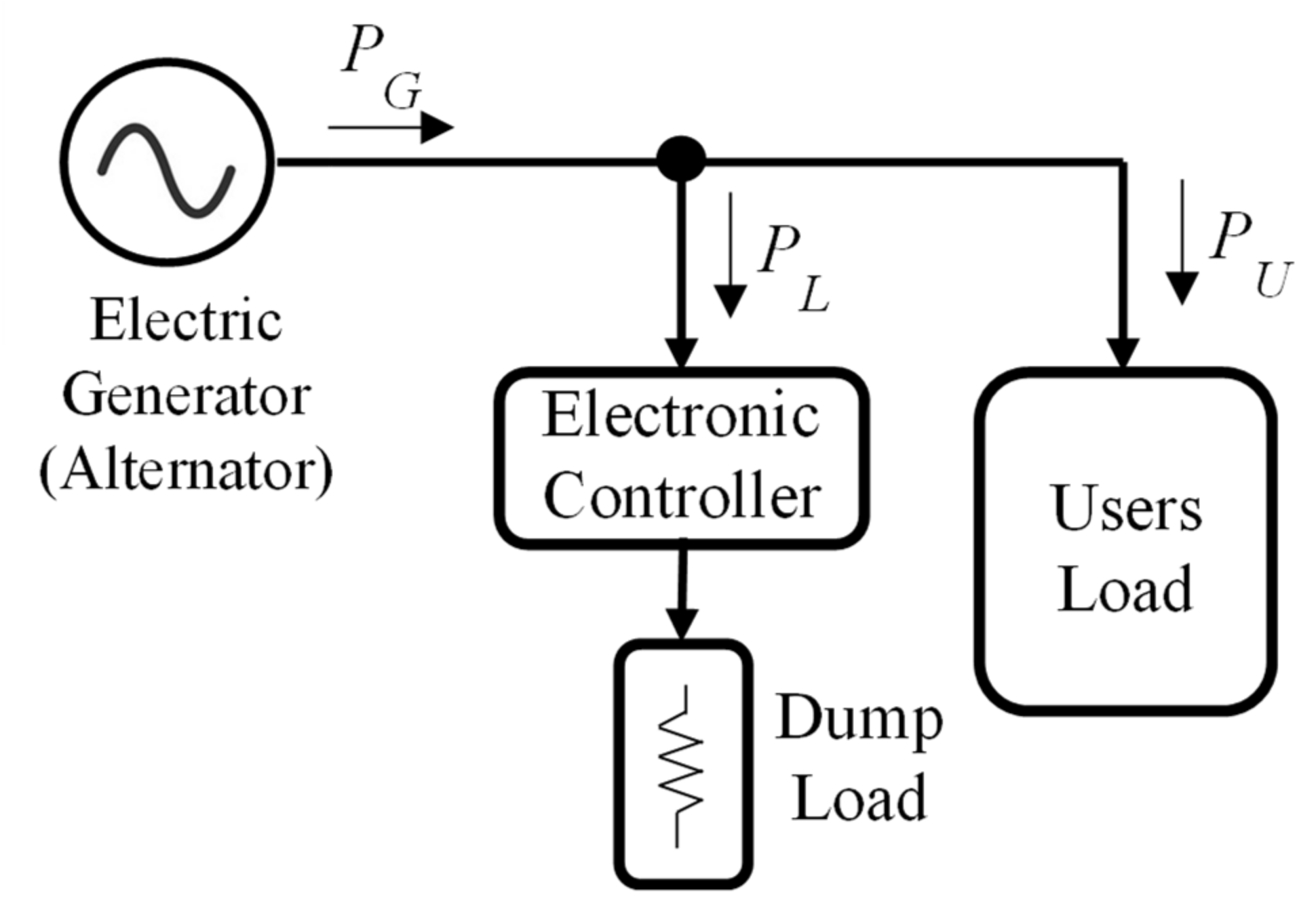
• The hydraulic turbine (prime mover), defined by Equation (1). Its inputs are volumetric water flow, the temperature and the position of the on/off valve. Its output is the mechanical power delivered by the turbine.
• The regulating frequency loop which is designed in deviation variable. It is built using the following blocks: Constant Set Point, whose value is cero to fix zero deviation around of the nominal frequency; Gcf(s), which represents the proportional integral (PI) frequency regulator with proportional gain Kprf and integral gain Kirf parameters; Alternator Mechanical Part Model, which represents the alternator mechanical model and whose mathematical expression is (7) relating ΔP_M, ΔP_U and ΔP_L with ΔF; and Krf that represent the gain of the frequency measurement device. The blocks From and Goto allow the signal interchange between different blocks of this scheme.
• The three-phase programmable voltage source, which represents the electric part of the alternator. It is used to feed both the user load and the converter.
• The user load, which represents the user’s load where are implemented different user consumption conditions employing the three-phase series load as physical component model.
• The converters, which is implemented using one of the topologies of converter as physical component model in order to simulate the converter under analysis. Its inputs are each one of the three phases, the Enable signal and the signal control sent by Gcf(s).

For frequency regulation, the PI regulator parameters were adjusted by applying the pole assignment method according to Cuban standard (NC62-04) requirements. These establish the maximum steady state error (E_SS) as 1% of the rated frequency, while the maximum overshoot (M_P) must not exceed ±1 Hz and the settling time must be less than 5 s. Those requirements were fulfilled by choosing a damping ratio (ξ) of 0.707 and an undamped natural frequency (wn) of 10 rad/s. Thus, the following constants were obtained:

$$K_{prf}=\frac{2\xi w_n{T}_G-1}{K_C{K}_G{K}_{rf}}=11.79 \mathrm{and} K_{irf}=\frac{w_n^2{T}_G}{K_C{K}_G{K}_{rf}}=83.35 s^{-1},$$

where K_C = 12000/5 = 2400 W/V, because Pmax was 12.0 kW and Mmax was 5 V, K_G = 0.3 Hz/W, T_G = 600.1 s and,

$$K_{rf}=\frac{U_{rfmáx}-U_{rfmín}}{F_{máx}-F_{mín}}=\frac{10 V-0 V}{65 Hz-55 Hz}=1 V/Hz.$$

4. Evaluation of the Frequency Regulation Loop

To evaluate the effect of rectifier topologies with symmetrical switching in the frequency regulation loop, the ‘Los Gallegos’ μHPP was used as a case study. Thus, we compared the proposed rectifier and symmetrical switching to the current AC-AC converter scheme.

The μHPP ‘Los Gallegos’ is a standalone μHPP having only the primary frequency regulation loop by ELC and its main system component parameters were:

• Rated power of the hydraulic turbine: 12.0 kW.
• Alternator voltage and frequency: 110 V RMS, 60 Hz.
• Rated speed: 1200 rpm.
• Number of poles: 6.
• Coefficient of friction by windage: 0.0063 N⋅m⋅s/rad.
• Turbine and alternator moment of inertia: 7.60 kg⋅m².

The frequency transducer operates with an input range from 55 to 65 Hz, giving an output range from 0 to 10 V. The minimum and maximum power consumed by users was 3.0 kW and 12.0 kW, respectively. The average value of sustained load power was about 3.0 kW, and the maximum value of sustained power consumption was 4 kW.

To simulate actual operation at the Los Gallegos μHPP, stepwise changes in consumer loads were introduced, as follows: at t = 3.0 s, the power was reduced by 3.0 kW and 2.5 kvar; at t = 5.0 s, the power was reduced by 3.0 kW and 3.0 kvar; and at t = 6.5 s, the consumption was increased by 4.0 kW and 3.5 kvar. This sequence emulates the typical variation in user consumption and helped us to assess the effects of the different ELCs on the frequency regulation performance.

4.1. Test Results with AC-AC Converters As Electronic Load Controllers

Figure 6 shows the changes in the instantaneous frequency when AC-AC converters were used as ELCs.

When the changes were introduced, as shown in Figure 6, the maximum deviation of the frequency from its rated value was less than 0.1 Hz and the steady state error was zero. The signal plotted shows that the settling time was less than 5 s, while the maximum error was 0.075 Hz, which corresponds to 7.5% of the M_P allowed by the Cuban standard.

The graphs in Figure 6 show that the requirements of the NC62-04 were met with the adjustment made to the regulator, while Figure 7 shows the behavior of the indices over time; the active power P_Gen, P_AC-AC, and P_U; the reactive power Q_Gen, Q_AC-AC, and Q_U, and power factor fp_Gen, fp_AC-AC, and fp_U were measured at the alternator output terminals, input terminals of the three AC-AC converters, and for the user load, respectively.

Figure 7a shows that, at the steady state corresponding to the time from t = 3.0 s to t = 5.0 s, P_AC-AC = 3 kW, compensating the decrement of P_U, that it is accomplished for α = 1.99 rad for which the signal sent by the frequency regulator M is 1.84 V, obtained from (14). For the steady state corresponding to the time from t = 5.0 s to t = 6.5 s, P_AC-AC = 6 kW, to compensate the next reduction of P_U, that is accomplished for α = 1.57 rad with the signal sent by the frequency regulator M = 2.50 V obtained from (14). Finally, after of the transient corresponding on the interval from t = 6.5 s to t = 8.0 s P_AC-AC = 2 kW because P_U = 10 kW. The power consumed by the set of three AC-AC converters must be 2 kW, the α must be 2.16 rad and, from (14), a value of M = 1.57 V is obtained. The previous discussion proves that the P_Gen is always equal to P_AC-AC plus P_U. The sum was 12 kW at a steady state, which demonstrates that both the AC-AC converters used as the ELC and the designed regulator achieved the frequency regulation.

Figure 7b shows that the alternator had to supply a reactive power, Q_Gen, greater than Q_U, because of Q_AC-AC. This verifies that, although the frequency was regulated with AC-AC converters, their reactive power consumption affected the alternator.

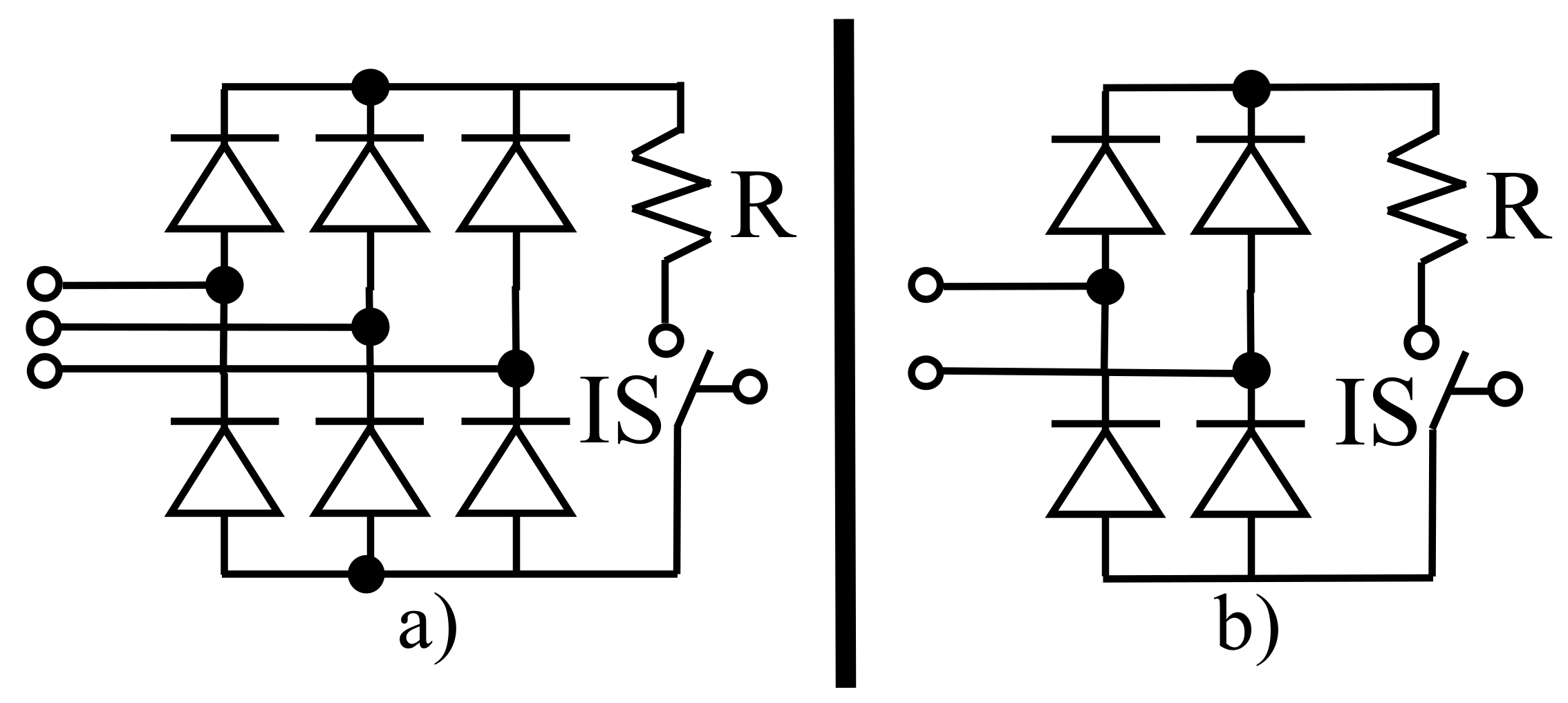
4.2. Test Results with the Three-Phase Rectifier with Symmetrical Switching as Electronic Load Controllers

Figure 8 shows the changes in the instantaneous frequency when a three-phase rectifier with symmetrical switching was used as the ELC. When power steps were introduced, the maximum deviation of the frequency from its rated value was less than 0.1 Hz and the steady state error was zero; the settling time was less than 5 s. In this case, the maximum error was 0.095 Hz, which corresponded to 9.5% of the M_P allowed by the Cuban standard. Thus, the graph shows that the requirements of NC62-04 were also met with these regulator adjustments.

Figure 9 shows the time behavior of active power P_Gen, P_Rect3, and P_U, reactive power Q_Gen, Q_Rect3, and Q_U and the power factor fp_Gen, fp_Rect3, and fp_U measured at the alternator output terminals, input terminals of the three-phase rectifier, and the user load, respectively.

Figure 9a shows that, at the steady state corresponding to the time from t = 3.0 s to t = 5.0 s, P_Rect3 = 3 kW, compensating the decrement of P_U, that it is accomplished for α = 0.40 rad for which the signal sent by the frequency regulator M is 1.15 V, obtained from (26). For the steady state corresponding to the time from t = 5.0 s to t = 6.5 s, P_Rect3 = 6 kW, to compensate the next reduction of P_U, that is accomplished for α = 0.28 rad with the signal sent by the frequency regulator M = 2.33 V obtained from (26). Finally, after the transient corresponding on the interval from t = 6.5 s to t = 8.0 s, P_Rect3 = 2 kW because P_U = 10 kW. The power consumed by the three-phase rectifier must be 2 kW, α must be 0.44 rad and from (26) M = 0.77 V is obtained. The previous discussion proves the P_Gen is always equal to P_Rect3 plus P_U. The sum was 12 kW at steady state, which demonstrates that both the three-phase rectifier used as the ELC and the designed regulator achieved the frequency regulation.

Figure 9b shows that the alternator had to supply a reactive power, Q_Gen, equal to Q_U, because Q_Rect3 was zero. Thus, we verified that unlike the ELC with AC-AC converters (Figure 7b), the frequency was regulated, and the reactive power delivered by the alternator was reduced with a three-phase rectifier such as the ELC. Therefore, the power factor at the alternator output terminals was improved with the three-phase rectifier with symmetrical switching, as shown by comparing the power factor at the alternator output terminals, the fp_Gen variable, in Figure 7c and Figure 9c.

Figure 10 shows the RMS current of an alternator phase when the AC-AC converters, Irms_GenAC-AC, or the three-phase rectifier, Irms_GenRect3, were used as ELCs. The figure shows that Irms_GenRect3 was smaller than Irms_GenAC-AC, even at a maximum of 4 A. Thus, by using the three-phase rectifier, the capacity of the alternator to deliver the current was increased because of the increase in the power factor at the alternator output terminals created by reducing the reactive consumption. As discussed above, using the three-phase rectifier increased the power factor at the alternator output terminals and also increased the capacity of the alternator in terms of the current it could deliver. These features all represent improvements over the current AC-AC ELC.

4.3. Test Results with the Set of Three Single-Phase Rectifiers with Symmetrical Switching as the Electronic Load Controller

Figure 11 shows the changes in the instantaneous frequency when the set of three single-phase rectifiers with symmetrical switching was used as the ELC.

When changes were introduced, as shown in Figure 11, the maximum deviation of the frequency from its rated value was less than 0.1 Hz, the steady state error was zero, and the settling time was less than 5 s. In this case, the maximum error was 0.068 Hz, which corresponds to 6.8% of the M_P allowed by the Cuban standard. These results mean that the requirements of the NC62-04 were met with the adjustments we made to the regulator.

Figure 12 shows the time behavior of active power P_Gen, P_3Rect1, and P_U, reactive power, Q_Gen, Q_3Rect1, and Q_U and the power factor fp_Gen, fp_3Rect1, and fp_U measured at the alternator output terminals, input terminals of three single-phase rectifiers, and the user load, respectively.

Figure 12a shows that, at the steady state corresponding to the time value from t = 3.0 s to t = 5.0 s, P_3Rect1 = 3 kW, compensating the decrement of 3 kW of the P_U, that it is accomplished for α = 1.37 rad for which the signal sent by the frequency regulator M is 0.7 V, obtained from (20). For the steady state belonging to the interval time from t = 5.0 s to t = 6.5 s, P_3Rect1 = 6 kW, to compensate the next reduction of P_U, that is accomplished for α = 1.15 rad with the signal sent by the frequency regulator M = 1.33 V obtained of (20). Finally, after the transient corresponding on the interval from t = 6.5 s to t = 8.0 s, P_3Rect1 = 2 kW because P_U = 10 kW. The power consumed by the set of three single-phase rectifiers must be 2 kW, α must be 1.44 rad and from (20) M = 0.43 V is obtained. The discussion proves that the P_Gen is always equal to P_3Rect1 plus P_U. The sum was 12 kW at steady state, which demonstrates that both the set of three single-phase rectifiers used as the ELC and the designed regulator achieved the frequency regulation.

Figure 12b shows that the alternator must supply a reactive power, Q_Gen, equal to Q_U, because Q_3Rect1 was zero. It verifies that, unlike ELCs with AC-AC converters (Figure 7b), by using single-phase rectifiers as the ELC, the frequency was regulated, and the reactive power delivered by the alternator was reduced. Therefore, with the set of three single-phase rectifiers with symmetrical switching, the power factor at the alternator terminals was improved, as can be seen by comparing the power factor at the alternator output terminals, the fp_Gen variable, in Figure 7c and Figure 12c.

Figure 13 shows the RMS current of an alternator phase when AC-AC converters, Irms_GenAC-AC, or single-phase rectifiers, Irms_Gen3Rect1, were used as ELCs. This shows that the Irms_Gen3Rect1 was less than the Irms_GenAC-AC, even at a maximum of 4.5 A, indicating that when the set of three single-phase rectifiers was used, the capacity of the alternator in terms of current delivery was increased because of the increase in the power factor at the alternator terminals because of a reduction in reactive consumption.

The graphics of frequency vs. time for each topology analyzed, Figure 6, Figure 8 and Figure 11, show that, after every transient, the frequency regulation of f = 60 Hz is accomplished despite of the change on the user power consumption, which means that the signal error, Δf, at steady state is null.

Next, it will be proven that the PI regulator accomplishes that Δf tends to zero for disturbance produced by changing the user’s power consumption in step form. Changes in step form are chosen to consider abrupt changes due to load connection or disconnection. The closed loop transfer function (CLTF) of the frequency regulator system in deviation variables shows in Figure 5 is given by:

$$\Delta F\left(s\right)=\frac{-\frac{K_{prf}·s+K_{irf}}{s}{K}_c\frac{K_G}{T_{G}s+1}}{1+\frac{K_{prf}·s+K_{irf}}{s}{K}_c\frac{K_G}{T_{G}s+1}{K}_{rf}}\Delta Ref\left(s\right)+\frac{\frac{K_G}{T_{G}s+1}}{1+\frac{K_{prf}·s+K_{irf}}{s}{K}_c\frac{K_G}{T_{G}s+1}{K}_{rf}}\left(\Delta P_M\left(s\right)+\Delta P_U\left(s\right)\right)$$

(29)

where ΔRef(s) is the constant set point equal to zero, for that the first term of the right hand of (29) is null.

Here it is considered that the turbine delivers a constant power, hence ΔP_M is zero. Moreover, since $T_c\ll T_G$ only K_C is taken into account as model of the converters, then (29) turns into:

$$\Delta F\left(s\right)=\frac{\frac{K_G}{T_{G}s+1}}{1+\frac{K_{prf}·s+K_{irf}}{s}{K}_c\frac{K_G}{T_{G}s+1}{K}_{rf}}\Delta P_U\left(s\right)$$

(30)

Simplifying (30)

$$\Delta F\left(s\right)=\frac{K_G·s}{T_G{s}^2+\left(K_{prf}{K}_c{K}_G{K}_{rf}+1\right)s+K_{irf}{K}_c{K}_G{K}_{rf}}\Delta P_U\left(s\right)$$

(31)

Now, applying the final value theorem to find the value to which tends Δf(t) before changes $\Delta P_U\left(s\right)$ in step of amplitude $P_{US}$:

$$\underset{t\to \infty }{\lim }\Delta f\left(t\right)=\underset{s\to 0}{\lim }s·\frac{K_G·s}{T_G{s}^2+\left(K_{prf}{K}_c{K}_G{K}_{rf}+1\right)s+K_{irf}{K}_c{K}_G{K}_{rf}}\frac{P_{US}}{s}=0$$

(32)

Equation (32) shows that for changes in step form in ΔP_U, the Δf tends to zero, which implies that the frequency tends to 60 Hz (note that f = Δf + 60).

The same result is obtained for changes in step form of the power delivered by the turbine. This linear analysis demonstrates that the steady state error is null.

5. Conclusions

This present work shows that the use of three-phase and single-phase rectifiers with symmetrical switching increases both the power factor at the alternator output terminals and the capacity of the alternator to deliver current, thereby improving upon the AC-AC regulated ELCs currently used in Cuba. Our results demonstrate that the rectifier topologies and switching form we propose satisfied the frequency regulation requirements imposed by the NC62-04 Cuban standard while also increasing the power factor at the output terminal of the alternator and the current delivery capacity of the alternator. The latter two factors, with the proposed rectifiers using symmetrical switching as the ELC, are considered improvements to currently used ELCs with AC-AC regulators.

References

1. International Hydropower Association. 2018 Hydropower Status Report. Sector Trends and Insights. Available online: https://hydropower-assets.s3.eu-west-2.amazonaws.com/publications-docs/iha_2018_hydropower_status_report_4.pdf (accessed on 26 April 2021).
2. Yah, N.F.; Oumer, A.N.; Idris, M.S. Small scale hydro-power as a source of renewable energy in Malaysia: A review. Renew. Sustain. Energy Rev. 2017, 72, 228–239. [Google Scholar] [CrossRef] [Green Version]
3. Anaza, S.O.; Abdulazeez, M.S.; Yisah, Y.A.; Yusuf, Y.O.; Salawu, B.U.; Momoh, S.U. Micro Hydro-Electric Energy Generation—An Overview. Am. J. Eng. Res. (AJER) 2017, 6, 5–12. [Google Scholar]
4. Tkáč, Š. Hydro power plants, an overview of the current types and technology. SSP J. Civ. Eng. 2018, 13, 115–126. [Google Scholar] [CrossRef]
5. Bory, H.; Vazquez, L.; Martínez, H.; Majanne, Y. Symmetrical angle switched single-phase and three-phase rectifiers: Application to micro hydro power plants. IFAC-PapersOnLine 2019, 52, 216–221. [Google Scholar] [CrossRef]
6. Gasore, G.; Ahlborg, H.; Ntagwirumugara, E.; Zimmerle, D. Progress for On-Grid Renewable Energy Systems: Identification of Sustainability Factors for Small-Scale Hydropower in Rwanda. Energies 2021, 14, 826. [Google Scholar] [CrossRef]
7. Mehta, D.B.; Adkins, B. Transient torque and load angle of a synchronous generator following several types of system disturbance. Proc. IEE Part A Power Eng. 1960, 107, 61–74. [Google Scholar] [CrossRef]
8. Singh, R.R.; Kumar, B.A.; Shruthi, D.; Panda, R.; Raj, C.T. Review and experimental illustrations of electronic load controller used in standalone Micro-Hydro generating plants. Eng. Sci. Technol. Int. J. 2018, 21, 886–900. [Google Scholar] [CrossRef]
9. Kamble, S.V.; Akolkar, S.M. Load frequency control of micro hydro power plant using fuzzy logic controller. In Proceedings of the International Conference on Power, Control, Signals and Instrumentation Engineering (ICPCSI), Chennai, India, 21–22 September 2017; pp. 1783–1787. [Google Scholar] [CrossRef]
10. Singh, R.R.; Chelliah, T.R.; Agarwal, P. Power electronics in hydro electric energy systems—A review. Renew. Sustain. Energy Rev. 2014, 32, 944–959. [Google Scholar] [CrossRef]
11. Colak, I.; Kabalci, E.; Fulli, G.; Lazarou, S. A survey on the contributions of power electronics to smart grid systems. Renew. Sustain. Energy Rev. 2015, 47, 562–579. [Google Scholar] [CrossRef]
12. Anwer, N.; Siddiqui, A.S.; Anees, A.S. A lossless switching technique for smart grid applications. Int. J. Electr. Power Energy Syst. 2013, 49, 213–220. [Google Scholar] [CrossRef]
13. Wu, D.; Tang, F.; Dragicevic, T.; Vasquez, J.C.; Guerrero, J.M. Autonomous active power control for islanded AC microgrids with photovoltaic generation and energy storage system. IEEE Trans. Energy Convers. 2014, 29, 882–892. [Google Scholar] [CrossRef] [Green Version]
14. EL Yakine, N.; Menaa, K.; Tehrani, K.; Boudour, M. Optimal tuning for load frequency control using ant lion algorithm in multi-area interconnected power system. Intell. Autom. Soft Comput. 2019, 25, 279–294. [Google Scholar] [CrossRef]
15. Kazerani, M.; Tehrani, K. Grid of Hybrid AC/DC Microgrids: A New Paradigm for Smart City of Tomorrow. In Proceedings of the 2020 IEEE 15th International Conference of System of Systems Engineering (SoSE), Budapest, Hungary, 2–4 June 2020; pp. 175–180. [Google Scholar] [CrossRef]
16. Rai, S.K.; Rahi, O.P.; Kumar, S. Implementation of electronic load controller for control of micro hydro power plant. In Proceedings of the 2015 International Conference on Energy Economics and Environment (ICEEE), Greater Noida, India, 27–28 March 2015; pp. 1–6. [Google Scholar] [CrossRef]
17. Chan, J.; Lubitz, W. Electronic load controller (ELC) design and simulation for remote rural communities: A powerhouse ELC compatible with household distributed-ELCs in Nepal. In Proceedings of the 2016 IEEE Global Humanitarian Technology Conference (GHTC), Seattle, WA, USA, 13–16 October 2016; pp. 360–367. [Google Scholar] [CrossRef]
18. Kusakana, K. A survey of innovative technologies increasing the viability of micro-hydropower as a cost effective rural electrification option in South Africa. Renew. Sustain. Energy Rev. 2014, 37, 370–379. [Google Scholar] [CrossRef]
19. Ofosu, R.A.; Kaberere, K.K.; Nderu, J.N.; Kamau, S.I. Design of BFA-optimized fuzzy electronic load controller for micro hydro power plants. Energy Sustain. Dev. 2019, 51, 13–20. [Google Scholar] [CrossRef]
20. Bhattarai, R.; Adhikari, R.; Tamrakar, I. Improved Electronic Load Controller for three phase isolated micro-hydro generator. In Proceedings of the 5th International Conference on Power and Energy Systems, Kathmandu, Nepal, 28–30 October 2013; Available online: https://www.researchgate.net/publication/303190135_Improved_Electronic_Load_Controller_for_Three_Phase_Isolated_Micro-Hydro_Generator (accessed on 26 April 2021).
21. Salhi, I.; Doubabi, S.; Essounbouli, N.; Hamzaoui, A. Frequency regulation for large load variations on micro-hydro power plants with real-time implementation. Int. J. Electr. Power Energy Syst. 2014, 60, 6–13. [Google Scholar] [CrossRef]
22. Singh, P.D.; Sharma, A.; Gao, S. PWM based AC-DC-AC converter for an isolated hydro power generation with variable turbine input. In Proceedings of the ICEPE, Shillong, India, 1–2 June 2018. [Google Scholar] [CrossRef]
23. Singh, P.D.; Gao, S. An isolated hydro power generation using parallel asynchronous generators at variable turbine inputs using AC-DC-AC converter. In Proceedings of the IICPE, Jaipur, India, 13–15 December 2018. [Google Scholar] [CrossRef]
24. Riaz, M.H.; Yousaf, M.K.; Izhar, T.; Kamal, T.; Danish, M.; Razzaq, A.; Qasmi, M.H. Micro hydro power plant dummy load controller. In Proceedings of the 2018 1st International Conference on Power, Energy and Smart Grid (ICPESG), Mirpur Azad Kashmir, Pakistan, 12–13 April 2018; pp. 1–4. [Google Scholar] [CrossRef]
25. Murthy, S.S.; Hegde, S. 5.-Hydroelectricity. In Electric Renewable Energy Systems; Rashid, M.H., Ed.; Academic Press: London, UK, 2016; pp. 79–81. [Google Scholar]
26. Traxler-Samek, G.; Lugand, T.; Schwery, A. Additional Losses in the Damper Winding of Large Hydrogenerators at Open-Circuit and Load Conditions. IEEE Trans. Ind. Electron. 2010, 57, 154–160. [Google Scholar] [CrossRef]
27. Nuzzo, S.; Bolognesi, P.; Gerada, C.; Galea, M. Simplified Damper Cage Circuital Model and Fast Analytical–Numerical Approach for the Analysis of Synchronous Generators. IEEE Trans. Ind. Electron. 2009, 66, 8361–8371. [Google Scholar] [CrossRef]
28. Kundur, P. Power System Stability and Control; McGraw-Hill, Inc.: New York, NY, USA, 1994. [Google Scholar]
29. Dewan, S.; Slemon, G.; Straughen, A. Power Semiconductor Drives; Wiley: New York, NY, USA, 1984. [Google Scholar]
30. Doolla, S. Frequency Control in Isolated Small Hydro Power Plant. Handbook of Renewable Energy Technology; World Scientific Publishing Co. Pte. Ltd.: Singapore, 2011; Chapter 20. [Google Scholar] [CrossRef]
Figure 1. Electronic load controller (ELC) for frequency regulation.
Energies 14 03201 g001
Figure 2. Topologies with symmetrical switching; (a) a three-phase rectifier; and (b) single-phase rectifier.
Energies 14 03201 g002
Figure 3. Phase current (blue: alternating current–alternating current (AC-AC) converter; red: rectifier and symmetrical switching).
Energies 14 03201 g003
Figure 4. Functional diagram of a micro-hydro power plant.
Energies 14 03201 g004
Figure 5. Scheme implemented in MATLAB/Simulink®.
Energies 14 03201 g005
Figure 6. Frequency signal of the regulation loop with an AC-AC converter.
Energies 14 03201 g006
Figure 7. Graphics for (a) active power; (b) reactive power; and (c) the power factor with the AC-AC converter.
Energies 14 03201 g007
Figure 8. Frequency signal of the regulation loop with the three-phase rectifier.
Energies 14 03201 g008
Figure 9. Graphics for (a) active power; (b) reactive power; and (c) the power factor with three-phase rectifier and symmetrical switching.
Energies 14 03201 g009
Figure 10. Root mean square (RMS) current delivery by the alternator.
Energies 14 03201 g010
Figure 11. Frequency signal of the regulation loop with three single-phase rectifiers.
Energies 14 03201 g011
Figure 12. Graphics for (a) active power; (b) reactive power; and (c) the power factor with single-phase rectifiers and symmetrical switching.
Energies 14 03201 g012
Figure 13. Effective current delivery by the alternator.
Energies 14 03201 g013