
A Study on Wear and Friction of Passenger Vehicles Control Arm Ball Joints


Abstract
:1. Introduction
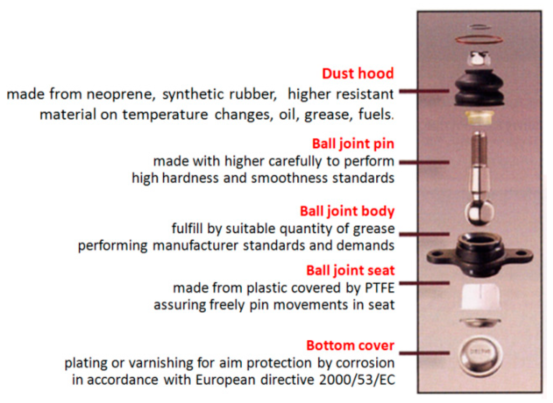
1.1. Ball Joint
- -
- Clunking noises from the car’s front suspension. The clearances between the worn ball joints and their socket increase. The joints start to rattle and knock during the up and down displacements of the suspension. Such joint knocks or clunks when traveling on rough roads, speed bumps, or when turning. The loudness of clunking increases with the wear of the ball joints or until they eventually completely fail and break.
- -
- Undue oscillations from the vehicle’s suspension. The loose worn ball joints vibrate excessively during driving. The vibrations stem from the affected ball joint from various sides of the car. Sometimes, the vibrations are felt via the steering wheel.
- -
- Wandering steering. The effect is that the vehicle steering drifts from one side to the other one on its own. When the ball joints operate efficiently, and the wheels are in good alignment, the steering wheel is simple and quick in response. Worn ball joints induce wandering of the car steering, requiring the driver to compensate. However, similar symptoms can also accompany the failures of control arm bushings [15], making the identification of the sound source difficult. The friction in the control arm ball joint can generate noise with high frequency in the order of several kHz, which can be difficult to hear by the driver or passengers.
1.2. Studies on Ball Joints
2. Materials and Methods
2.1. Measurement of the Chosen Geometrical Parameters of the Ball Joints
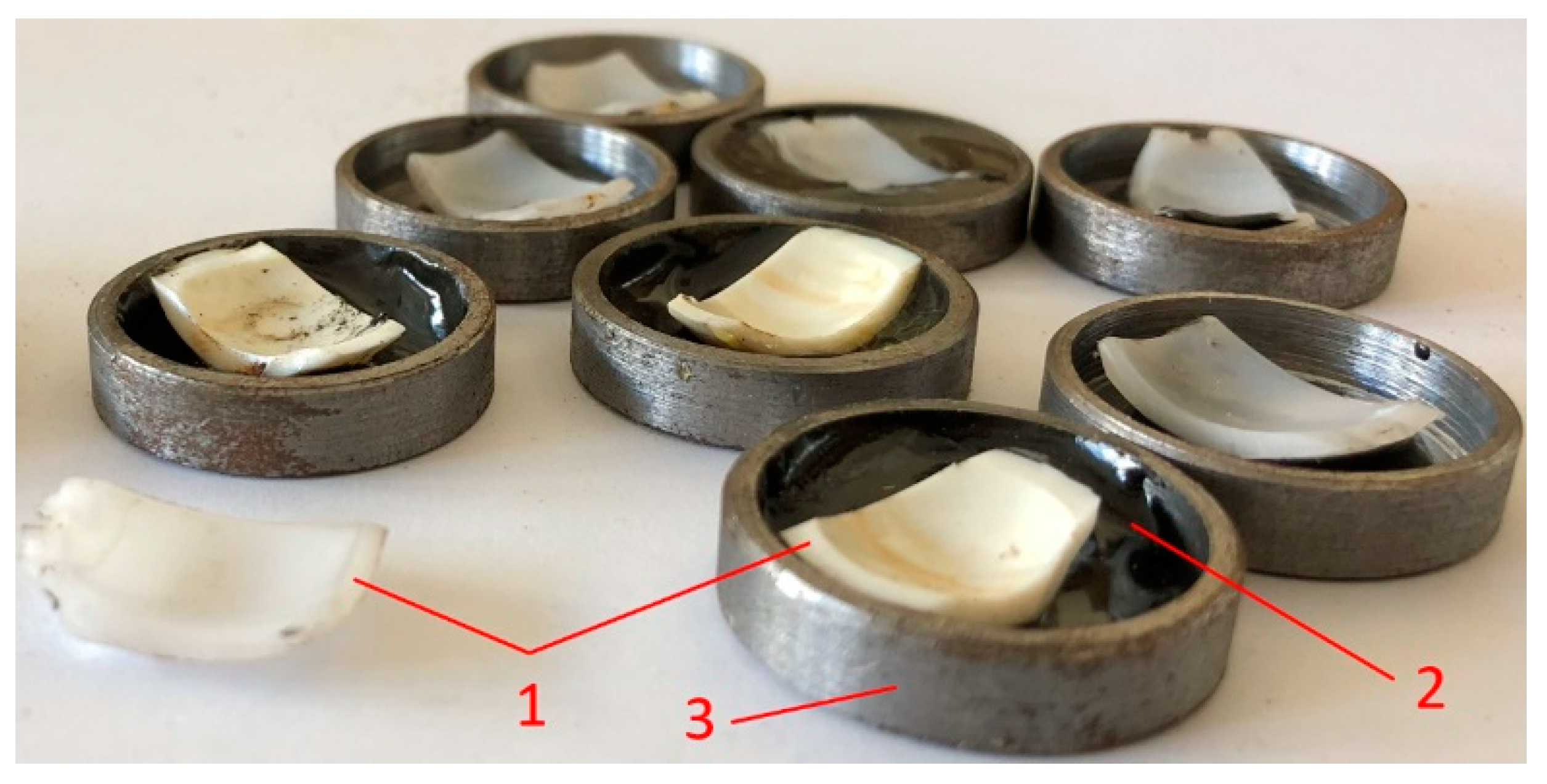
2.2. Experimental Determination of Material Models Parameters for Ball Joint Pin and Ball Joint Bearing
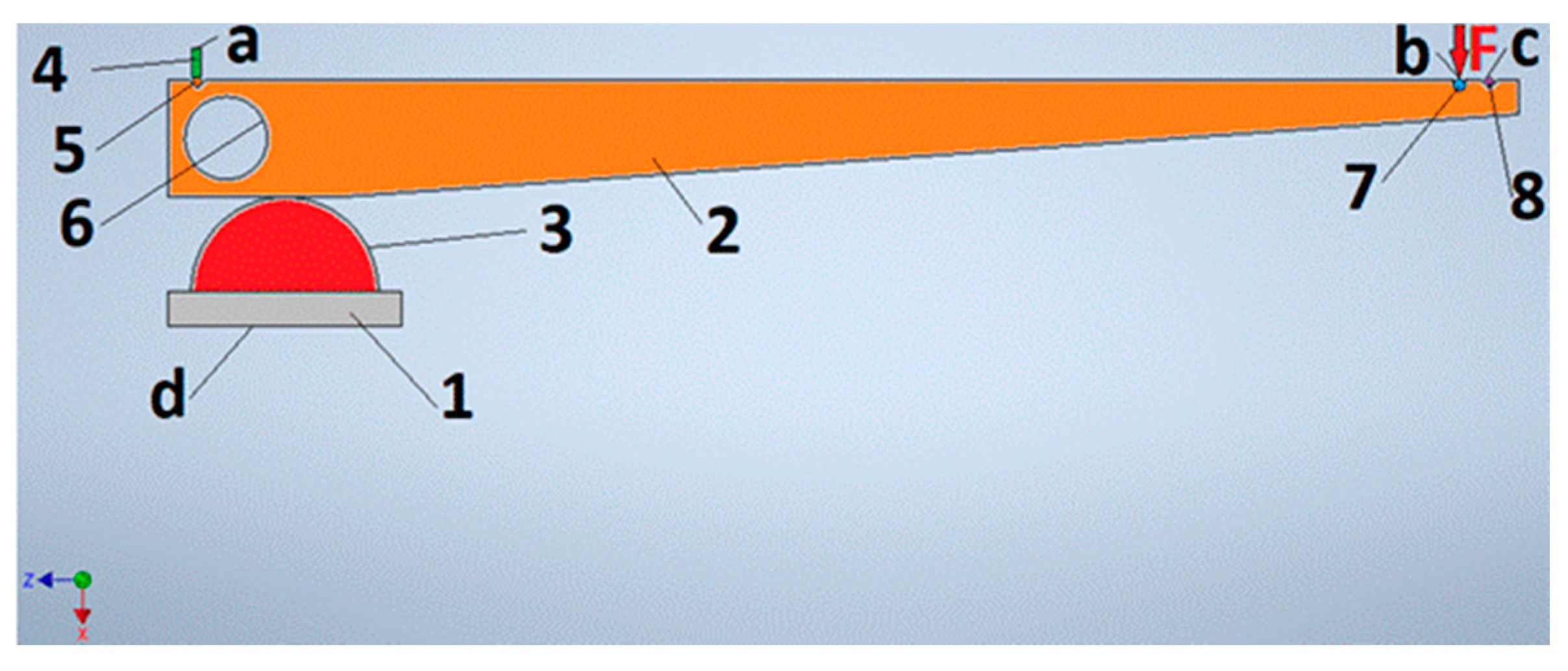
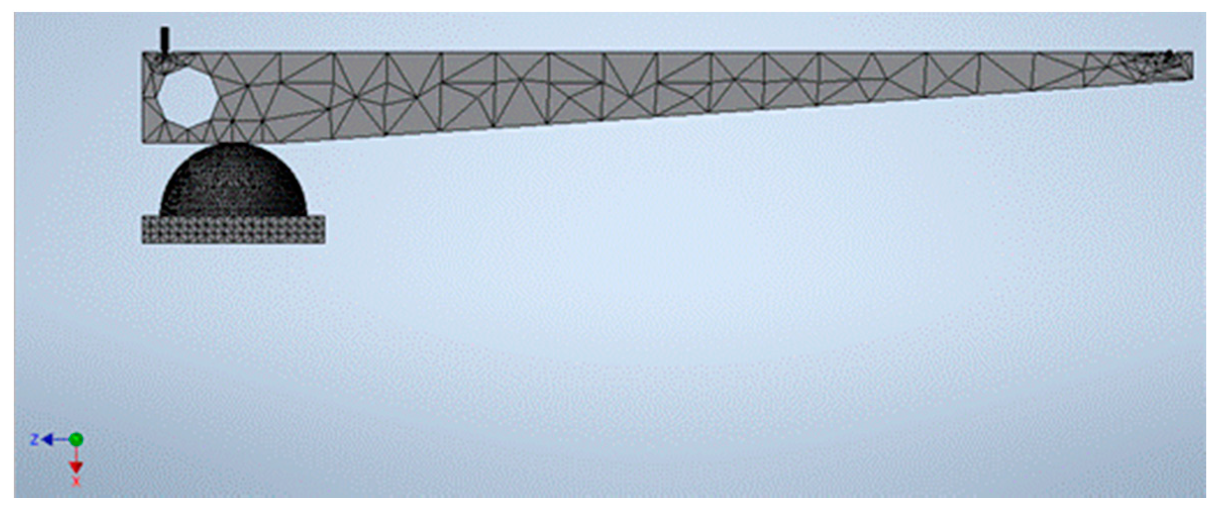
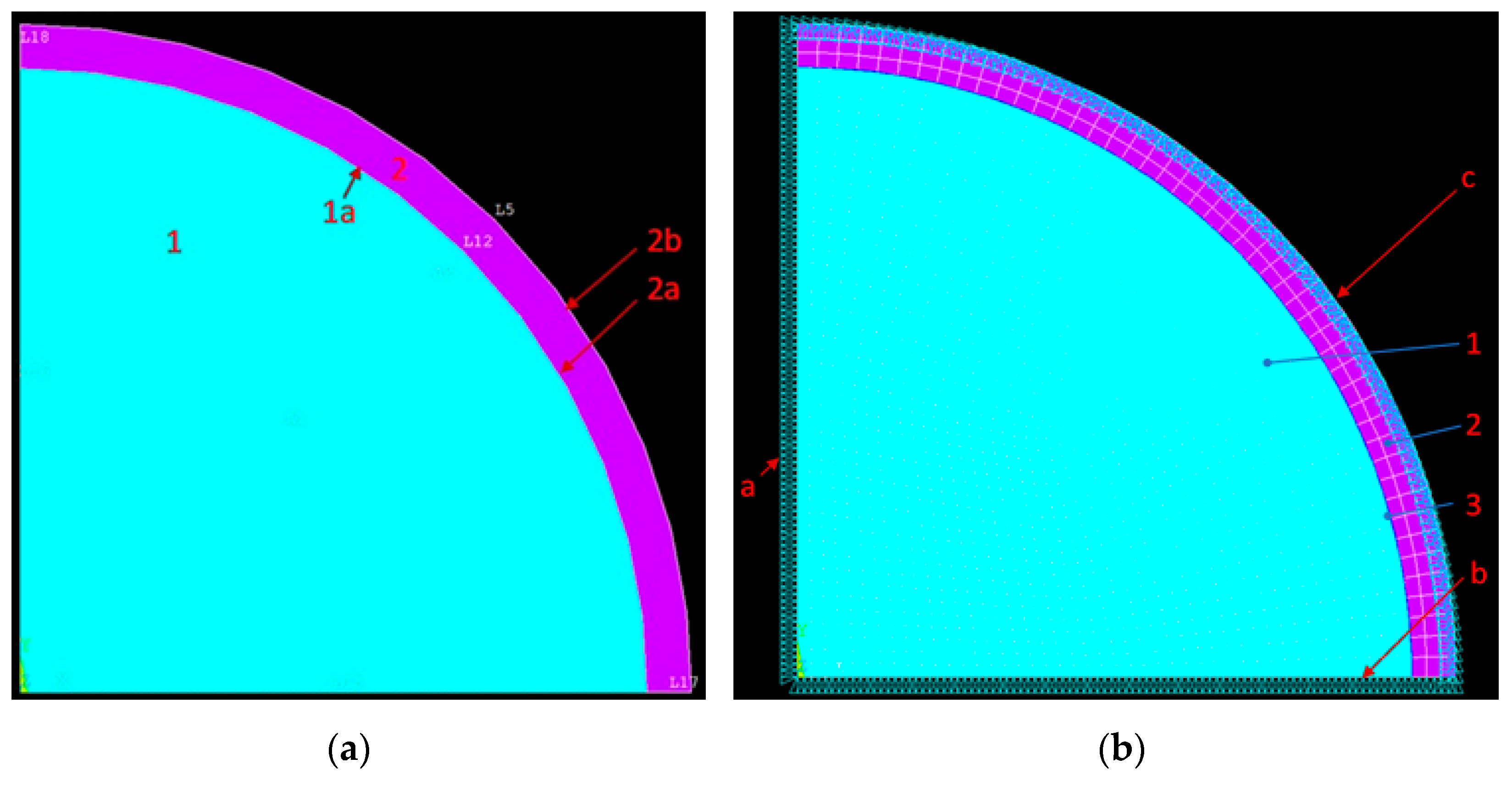
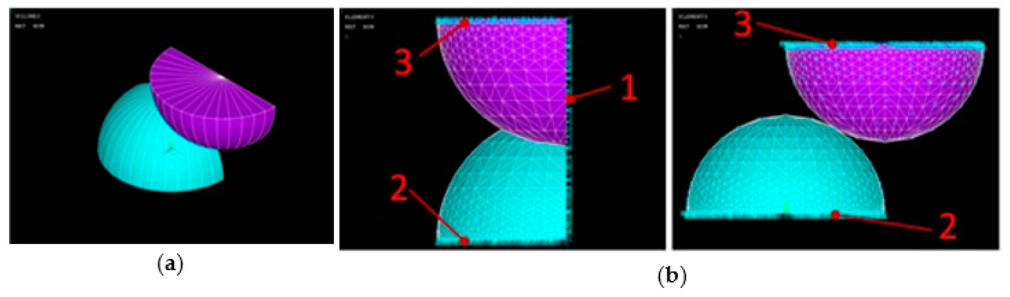
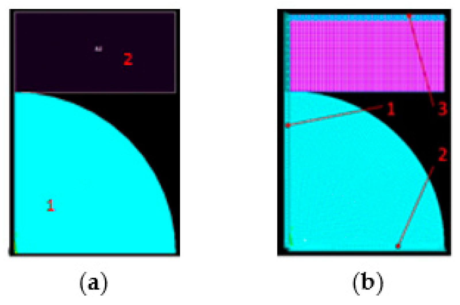
2.3. Numerical Determination of the Modeled Material Sample Deformations of the Ball Joint Bearing
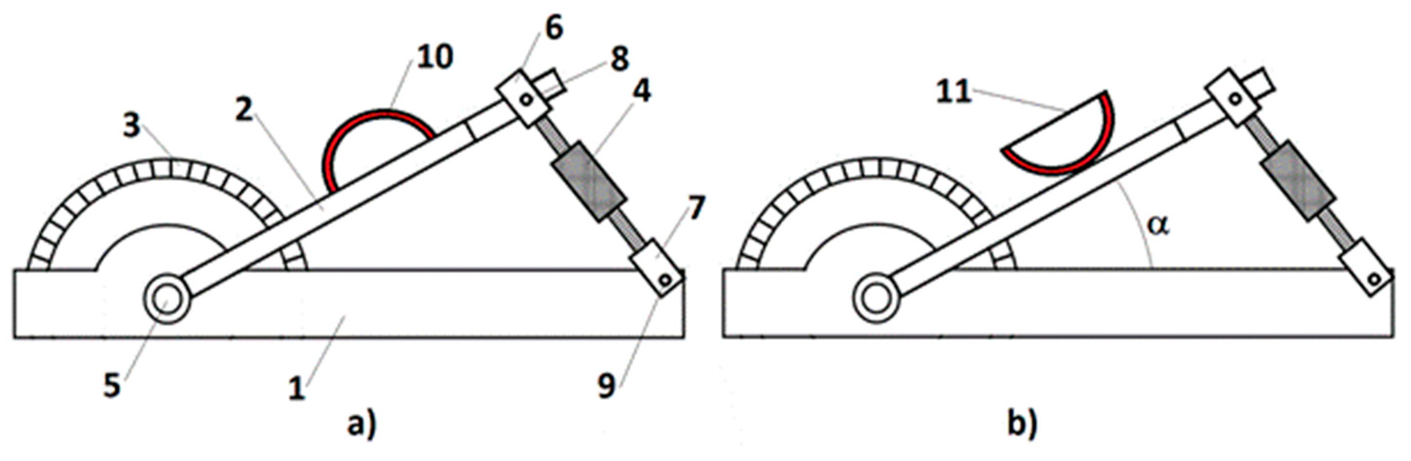
2.4. Friction Coefficient Determination between Steel and Ball Joint Bearing Material
2.5. Tribological Model
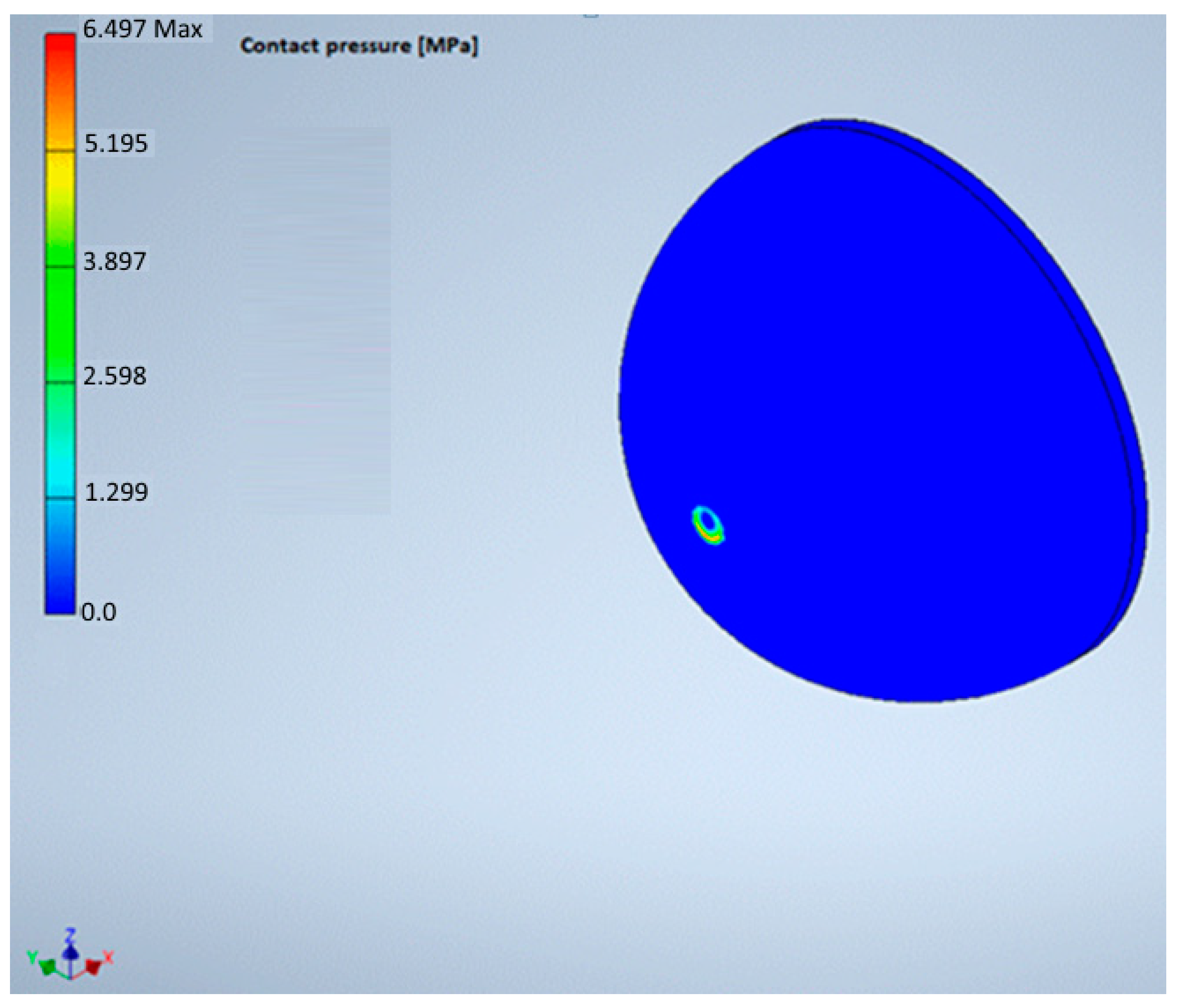
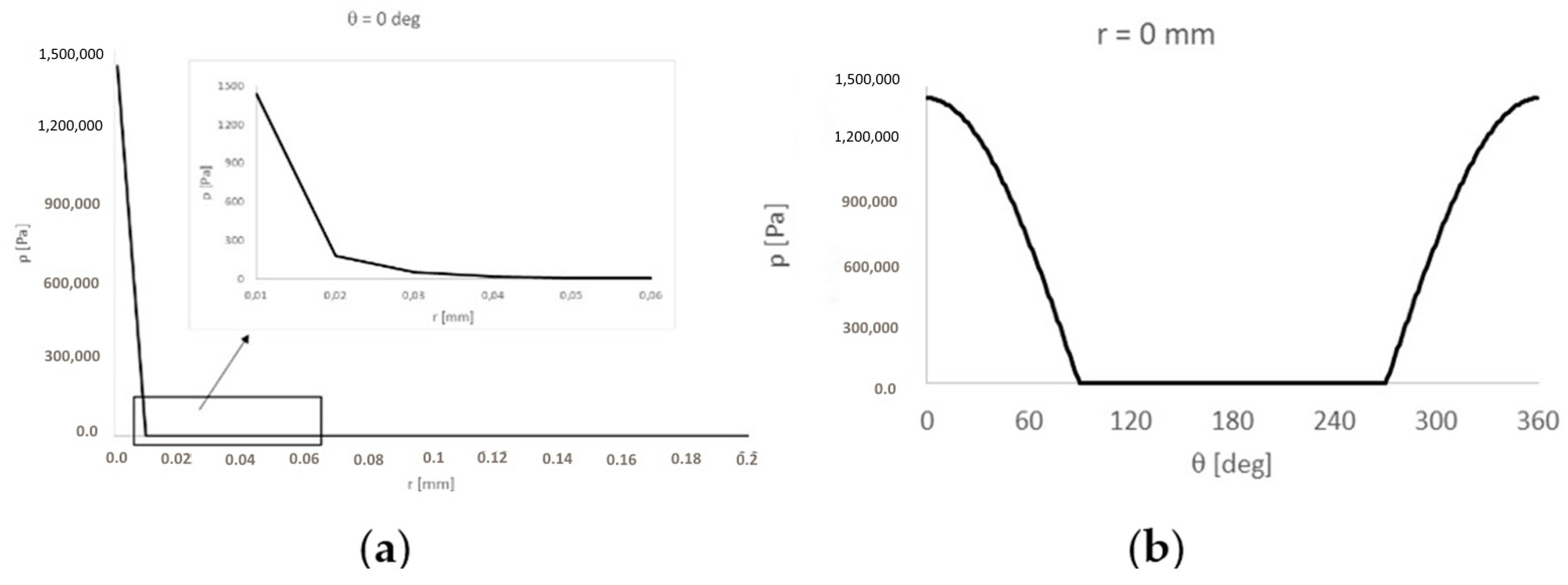
2.6. Contact Pressure Determination in the Zone between Ball Joint Pin and Its Bearing
2.7. Resistive Force Determination Generated Due to Bodies Deformation
2.8. Determination of Resistive Force Generated Due to Adhesion
2.9. Determination of Resistive Force Generated Due to Fluid Shear Stresses
3. Results
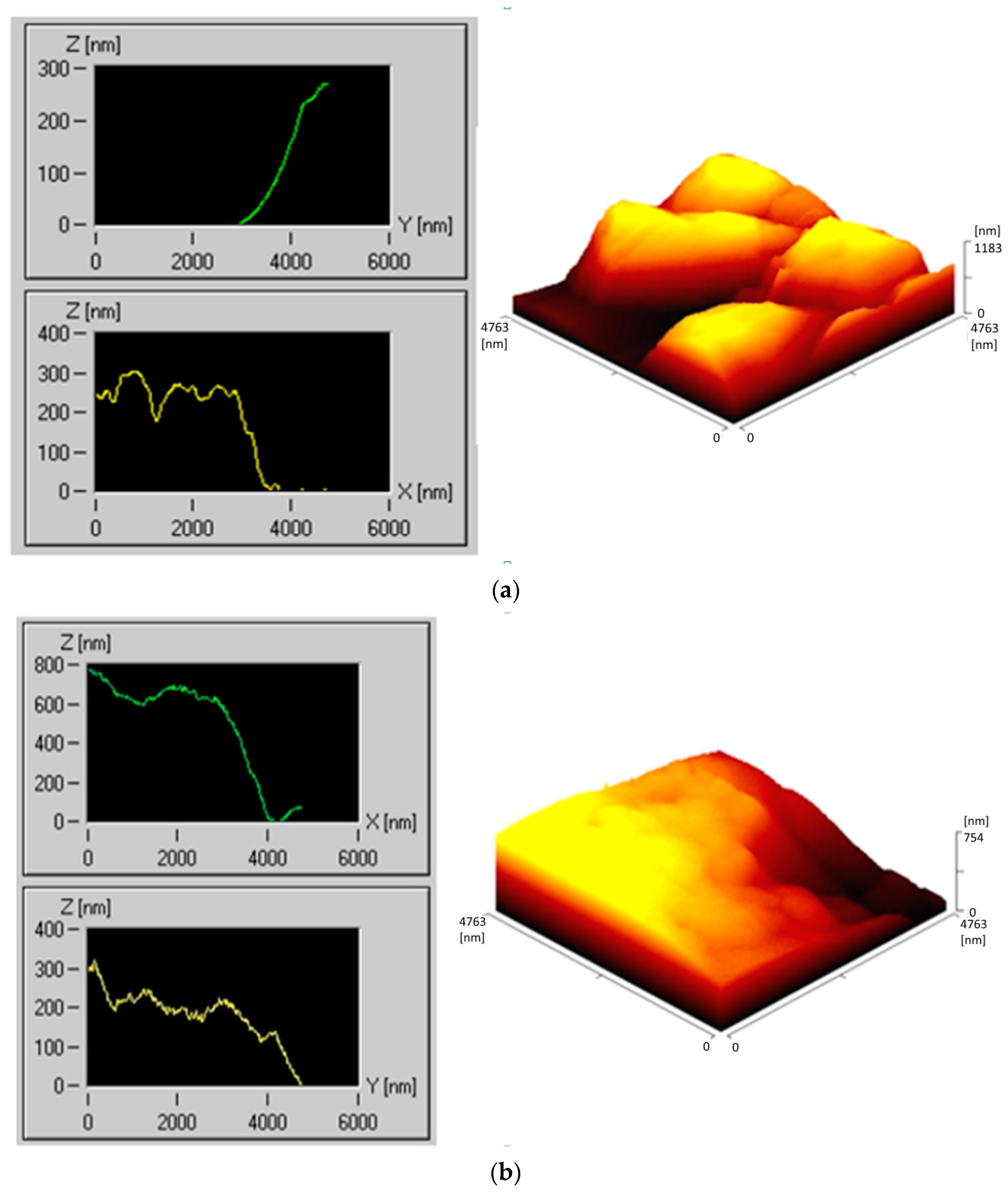
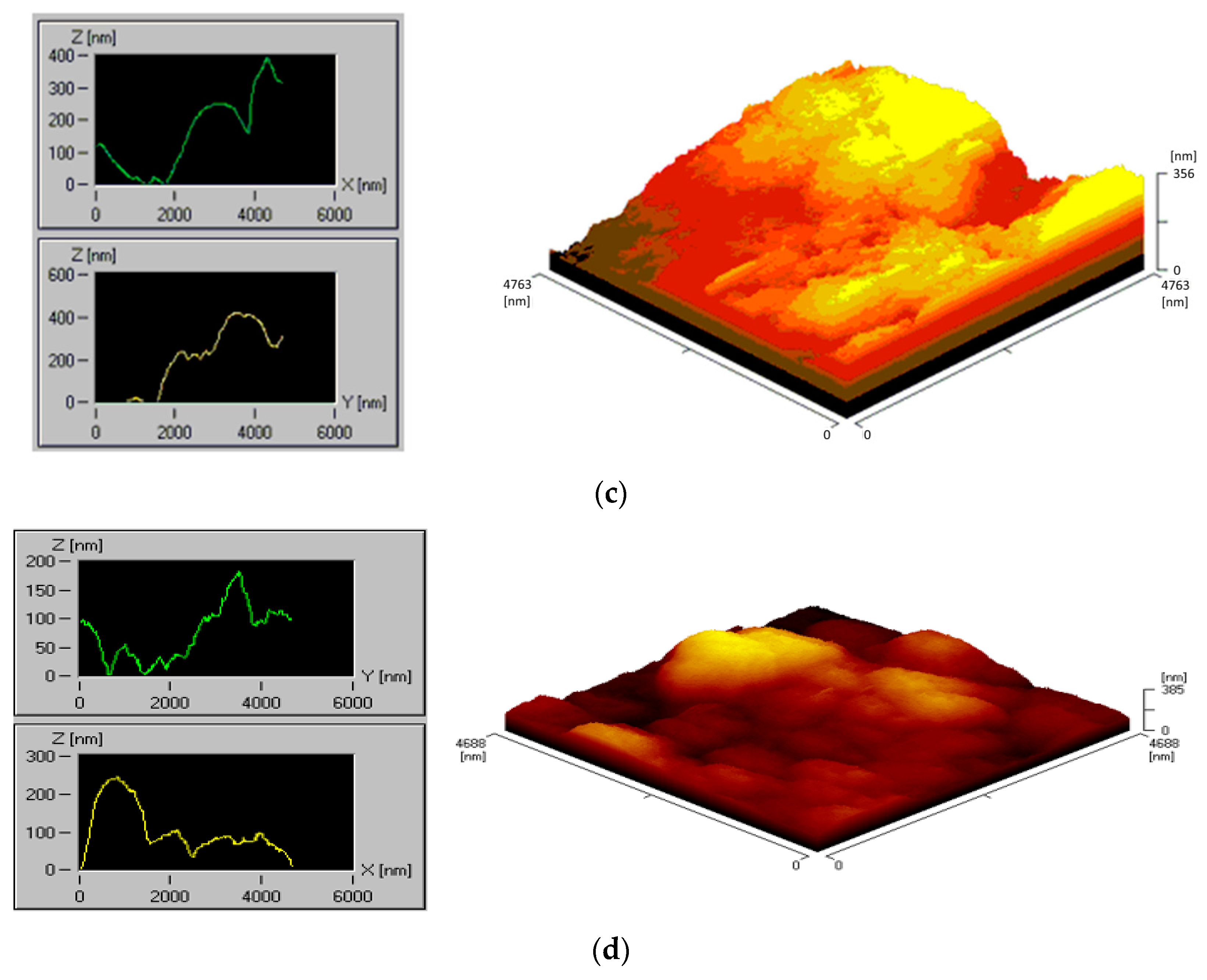
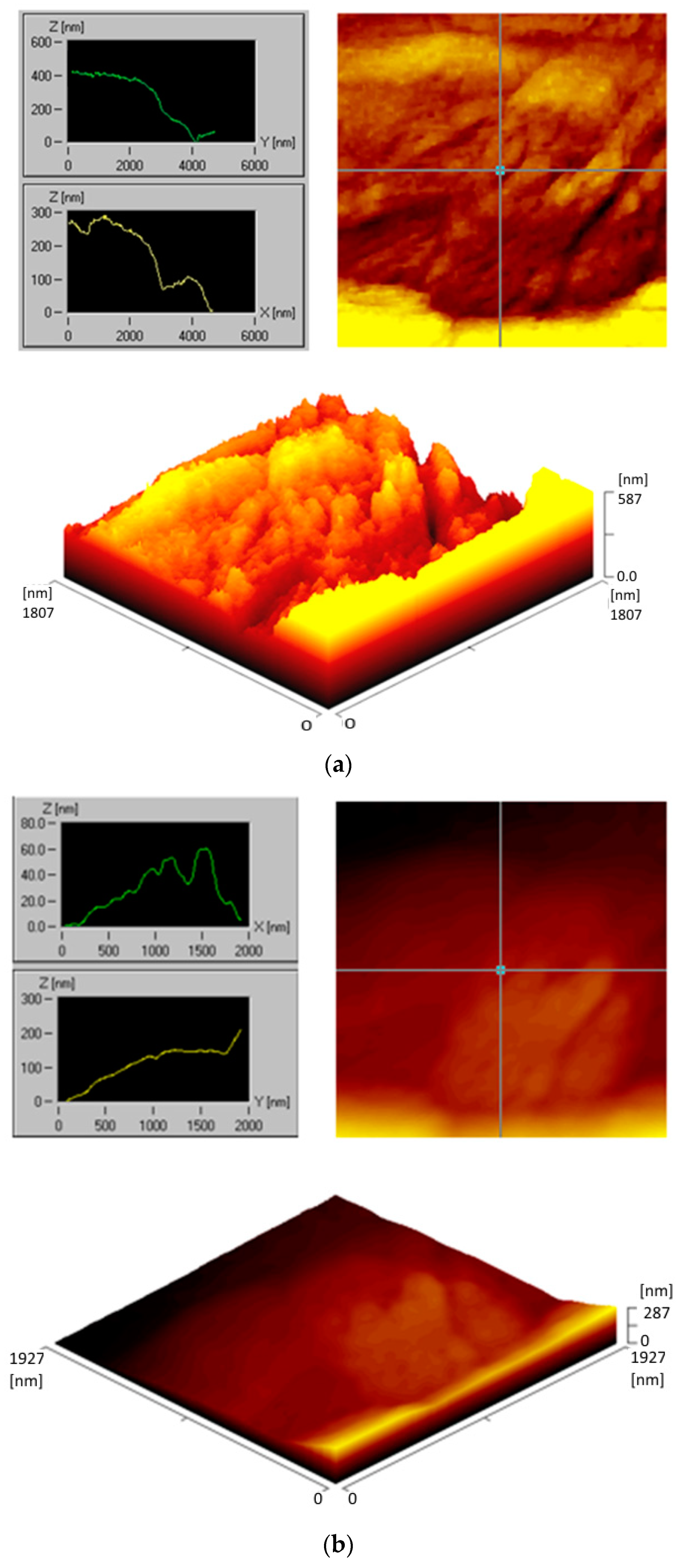
3.1. Ra Profile Measurements
3.2. Experimental Determination of Material Model Parameters
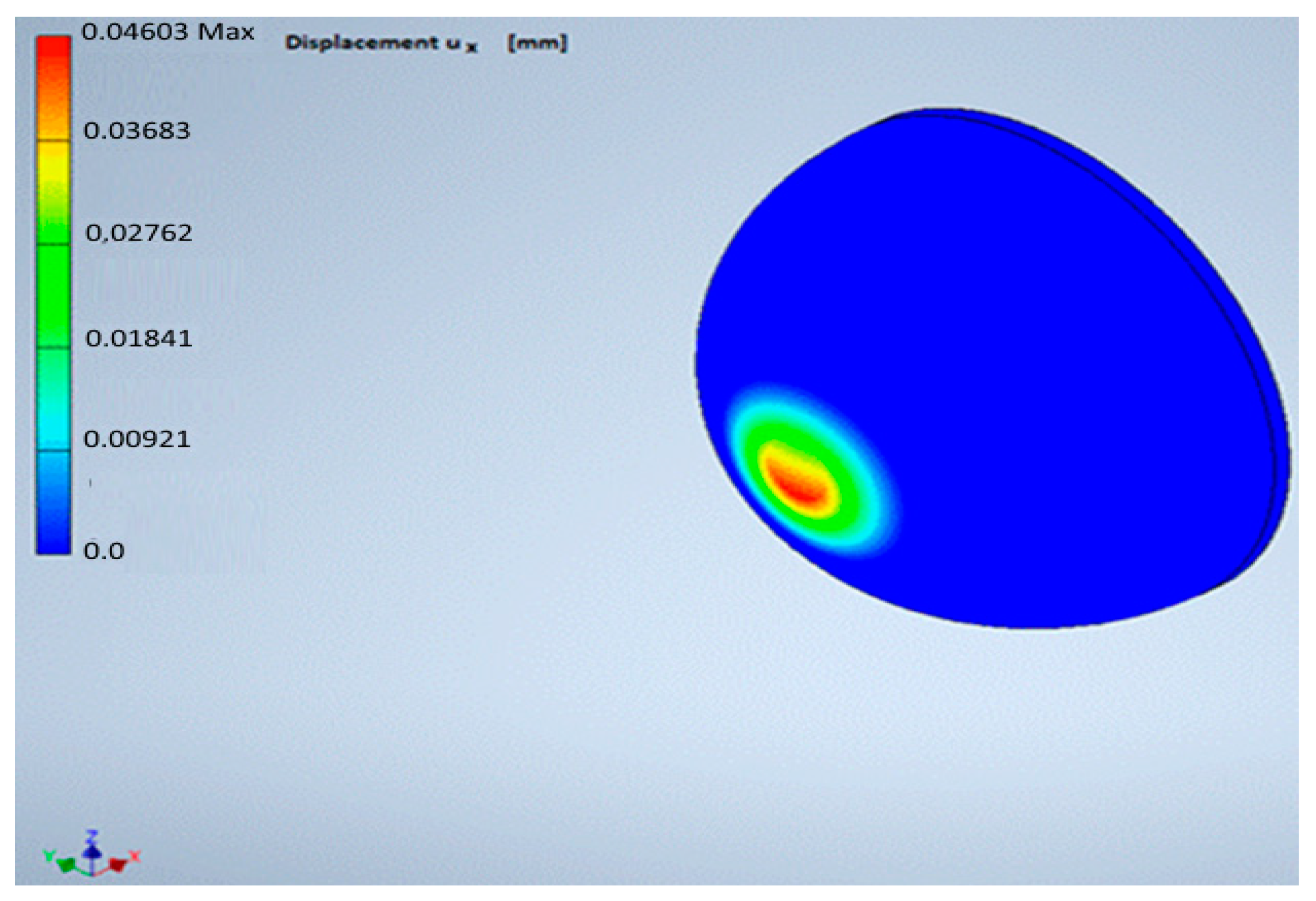
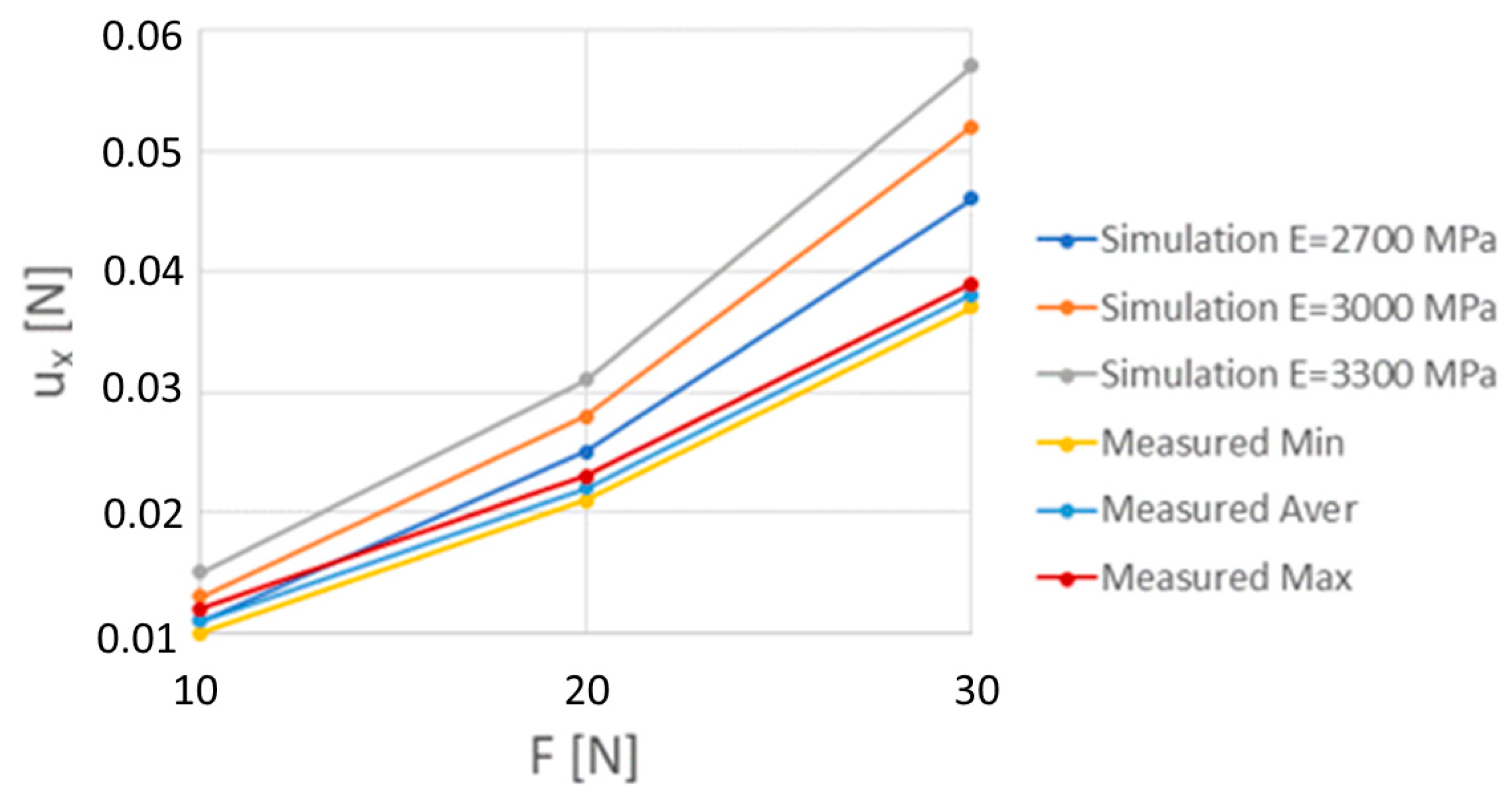
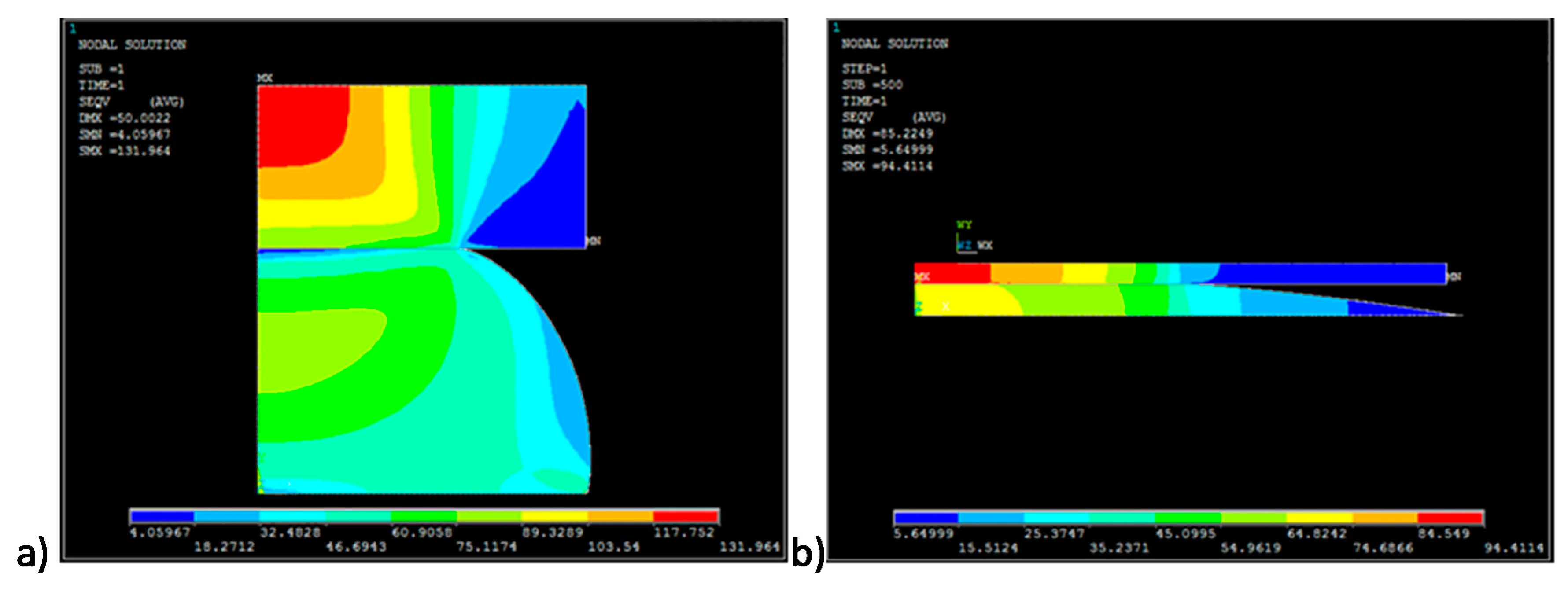
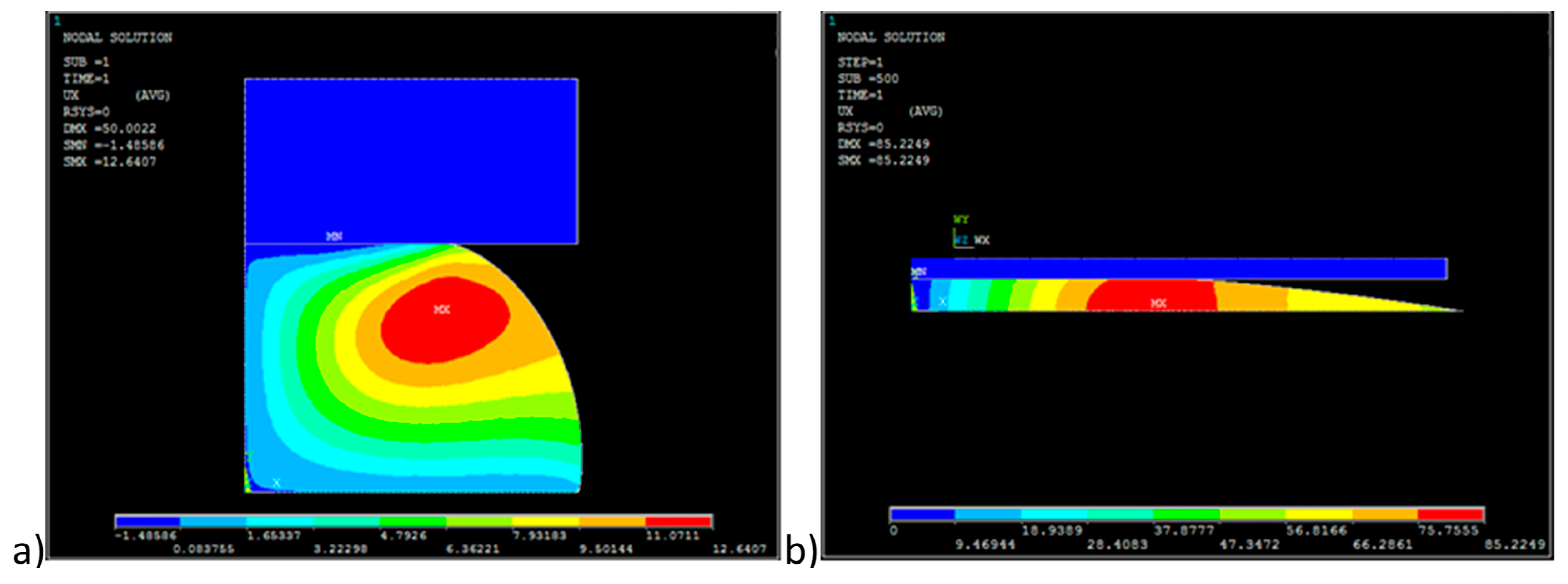
3.3. Numerical Determination of Ball Joint Bearing Deformations
3.4. Determination of Friction Coefficient between Steel and Ball Joint Bearing Material
3.5. Calculation Results of the Resistive Force and Torque in Ball Joint
4. Conclusions
Author Contributions
Funding
Conflicts of Interest
References
- Wozniak, M.; Ozuna, G.; De La Fuente, P.; Jozwiak, P.; Pawelski, Z. Test bench with AFM and STM modules for wear researches passenger’s car suspensions elements. Int. Virtual J. Sci. Tech. Innov. Ind. MTM 2012, 4, 9–11. [Google Scholar]
- Patil, P.B.; Kharade, M.V. Finite Element Analysis and Experimental Validation of Lower Control Arm. Int. J. Eng. Dev. Res. 2016, 4, 1914–1922. [Google Scholar]
- Duffy, J.E. Modern Automotive Technology, 9th ed.; The Goodheart-Willcox Company: Tinley Park, IL, USA, 2017. [Google Scholar]
- Mondragon-Parra, E.; Ambrose, G. Influence of Grease in Mechanical Efficiency of Constant Velocity Joints; SAE Technical Paper; SAE International: Warrendale, PA, USA, 2016. [Google Scholar]
- Yao, J.; Wang, M.; Li, Z.; Jia, Y. Research on Model Predictive Control for Automobile Active Tilt Based on Active Suspension. Energies 2021, 14, 671. [Google Scholar] [CrossRef]
- Heißing, B.; Ersoy, M. Chapter 5. Ride Comfort and NVH. In Chassis Handbook; Heißing, B., Ersoy, M., Eds.; Vieweg + Teubner: Wiesbaden, Germany, 2011; pp. 421–448. [Google Scholar]
- Paulraj, M.P.; Yaacob, S.; Andrew, A.M. Vehicle noise comfort level indication: A psychoacoustic approach. In Proceedings of the 6th International Colloquium on Signal Processing & its Applications, Mallaca City, Malaysia, 21–23 May 2010; pp. 1–5. [Google Scholar]
- Chung, S.S.; Lee, Y.Z.; Park, S.O. Practical Evaluation of Ball Stud Plating Effects on the Increase of Free Gap of Ball Joints in the Vehicle. Int. J. Automot. Technol. 2020, 21, 1107–1111. [Google Scholar] [CrossRef]
- Wozniak, M.; Ozuna, G.; De La Fuente, P.; Jozwiak, P.; Pawelski, Z. Comparision of friction coefficient for selected car suspension elements. Int. Virtual J. Sci. Tech. Innov. Ind. MTM 2014, 4, 23–25. [Google Scholar]
- Kang, J. Theoretical model of ball joint squeak. J. Sound Vib. 2011, 330, 5490–5499. [Google Scholar] [CrossRef]
- Farfan-Cabrera, L.I. Tribology of electric vehicles: A review of critical components, current state and future improvement trends. Tribol. Int. 2019, 138, 473–486. [Google Scholar] [CrossRef]
- Zhang, J.; Wang, D.; Chen, W. The application of PTFE coating on spherical joints. In Proceedings of the 2nd International Conference on Machinery, Materials Engineering, Chemical Engineering and Biotechnology, Chongqing, China, 28–29 November 2015. [Google Scholar]
- Komori, K.; Nagataki, T. Friction behavior of diamond-like carbon coated ball joint: Approach to improving vehicle handling and ride-comfort. SAE Int. J. Passeng. Cars-Mech. Syst. 2015, 8, 638–646. [Google Scholar] [CrossRef]
- Palange, N. Common Problems with Control Arm Bushings and How to Prevent Them. V&FAuto. 23 January 2018. Available online: https://vfauto.com/common-problems-control-arm-bushings-fix/ (accessed on 3 October 2020).
- Ossa, E.A.; Palacio, C.C.; Paniagua, M.A. Failure analysis of a car suspension system ball joint. Eng. Fail. Anal. 2011, 18, 1388–1394. [Google Scholar] [CrossRef]
- Symptoms of a Bad or Failing Ball Joint (Front). 2016. Available online: https://www.autoblog.com/2016/01/04/symptoms-of-a-bad-or-failing-ball-joint-front/ (accessed on 3 October 2020).
- Omar, S.B. Tribology study of suspension and linkages in automotive. Mytribos Symp. 2017, 2, 38–40. [Google Scholar]
- Muscă, I.; Românu, I.C.; Gagea, A. Preliminary study of friction in automotive ball joints. In Proceedings of the IOP Conference Series: Materials Science and Engineering, Proceedings of the International Conference on Tribology (ROTRIB’19), Cluj-Napoca, Romania, 19–21 September 2019; Volume 724. [Google Scholar]
- Watrin, J.-C.; Makich, H.; Haddag, B.; Nouari, M.; Grandjean, X. 23ème Congrès Français de M 23ème Congrès Français de Mécanique [CFM2017 Analytical modelling of the ball pin and plastic socket contact in a ball joint. In Proceedings of the Conference Proceedings, Lille, France, 28 August–1 September 2017. [Google Scholar]
- Sahu, D.P.; Singh, M.K.; Singh, S.; Sahu, N.K. Dynamics Analysis of Frictionless Spherical Joint with Flexible Socket. In Innovative Product Design and Intelligent Manufacturing Systems. Lecture Notes in Mechanical Engineering; Deepak, B., Parhi, D., Jena, P., Eds.; Springer: Singapore, 2020. [Google Scholar]
- Sin, B.-S.; Lee, K.-H. Process Design of a Ball Joint, Considering Caulking and Pull-Out Strength. Sci. World J. 2014, 2014, 971679. [Google Scholar] [CrossRef]
- Sun, Z.; Hao, C. Conformal Contact Problems of Ball-socket and Ball. Phys. Procedia 2012, 25, 209–214. [Google Scholar] [CrossRef] [Green Version]
- Koumura, S.; Shionoya, T. Ride comfort analysis considering suspension friction with series rigidity. SAE Int. J. Passeng. Cars-Mech. Syst. 2016, 9, 409–418. [Google Scholar] [CrossRef]
- Rutci, A.; Eren, S. Investigation of Suspension Ball Joint Pull Out Force Based on FEA Method and Experimental Study. In Proceedings of the 6th International Symposium on Innovative Technologies in Engineering and Science, Alanya, Turkey, 9–11 November 2018. [Google Scholar]
- Yang, X. Effects of bushings characteristics on suspension ball joint travels. Veh. Syst. Dyn. 2011, 49, 181–197. [Google Scholar] [CrossRef]
- Burcham, M.N.; Escobar, R.; Yenusah, C.O.; Stone, T.W.; Berry, G.N.; Schemmel, A.L.; Watson, B.M.; Verzwyvelt, C.U. Characterization and Failure Analysis of an Automotive Ball Joint. J. Fail. Anal. Prev. 2017, 17, 262–274. [Google Scholar] [CrossRef]
- Dowson, D.; Wang, D. Impact elastohydrodynamics. In Tribology Series; Dowson, D., Taylor, C.M., Childs, T.H.C., Dalmaz, G., Eds.; Elsevier: Amsterdam, The Netherlands, 1995; Volume 30, pp. 565–582. [Google Scholar]
- Raj, V. Analysis of Ball Stud Plating Effects on Variations of Vacuum Gap of Ball Joints in the Automobile. Int. Res. J. Mod. Eng. Technol. Sci. 2020, 2, 3694474. [Google Scholar]
- Park, K.D.; Ryu, H.J. A study on corrosion characteristics of suspension material by surface processing. Trans. Korean Soc. Automot. Eng. 2005, 13, 17–23. [Google Scholar]
- Trapp, M.; Chen, F. Automotive Buzz, Squeak and Rattle, 1st ed.; Elsevier: Waltham, MA, USA, 2012. [Google Scholar]
- Marques, F.; Flores, P.; Claro, J.C.; Lankarani, H. Modeling and analysis of friction including rolling effects in multibody dynamics: A review. Multibody Syst. Dyn. 2018, 45, 223–244. [Google Scholar] [CrossRef]
- ASTM D7420—11: Standard Test Method for Determining Tribomechanical Properties of Grease Lubricated Plastic Socket Suspension Joints Using a High-Frequency, Linear-Oscillation (SRV) Test Machine; ASTM International: West Conshohocken, PA, USA, 2011.
- Weiss, C.; Morlock, M.M.; Hoffmann, N.P. Friction induced dynamics of ball joints: Instability and post bifurcation behavior. Eur. J. Mech. A Solids 2014, 45, 161–173. [Google Scholar] [CrossRef]
- High Performance Polymers. Available online: https://www.tribology-abc.com/abc/polymers.htm (accessed on 3 October 2020).
- Habel, O. Instationäre Mischreibungssimulation Konformer Stahl-Polymer-Kontakte unter Berücksichtigung von Mangelschmierungseffekten. Ph.D. Thesis, Ruhr-Universität Bochum, Bochum, Germany, 2013. [Google Scholar]
- Geren, N.; Osman, O.A.; Melih, B. Parametric design of automotive ball joint based on variable design methodology using knowledge and feature-based computer assisted 3D modelling. Eng. Appl. Artif. Intell. 2017, 66, 87–103. [Google Scholar] [CrossRef]
- Ansys v.19.3 Mechanical APDL Documentation. Available online: https://ansyshelp.ansys.com/account/secured?returnurl=/Views/Secured/corp/v193/ans_mat/amp8sq21dldm.html%23elemedp (accessed on 3 October 2020).
- Frédy, C. Modeling of the Mechanical Behavior of Polytetrafluoroethylene (PTFE) Compounds during Their Compaction at Room Temperature. Ph.D. Thesis, Université Pierre et Marie Curie, Paris, France, 2015. [Google Scholar]
- Clarhed, D. Stress Analysis of PTFE Sleeves in Industrial Valves; Lund University: Lund, Sweden, 2008. [Google Scholar]
- Bergstrom, J. Accurate Finite Element Simulations of PTFE Components; Veryst Engineering, LLC: Needham, MA, USA, 2012. [Google Scholar]
- Löfgrena, H.B. A solution to the hydrodynamic lubrication of a circular point contact sliding over a flat surface with cavitation. Theor. Appl. Mech. Lett. 2012, 2, 032004. [Google Scholar] [CrossRef] [Green Version]
- Woydt, M.; Schneider, A. Application oriented tribological test concepts. Lube Mag. 2020, 159, 22–28. [Google Scholar]
- Heißing, B.; Ersoy, M. Chassis Handbook. Fundamentals, Driving Dynamics, Components, Mechatronics, Perspectives; ATZ/MTZ-Fachbuch Series; Heißing, B., Ersoy, M., Eds.; Vieweg + Teubner Verlag, Springer: Berlin/Heidelberg, Germany, 2011. [Google Scholar]


| Force F [N] | Displacement [mm] | Displacement [mm] |
|---|---|---|
| 10 | 6.22 ± 0.01 | 0.011 ± 0.001 |
| 20 | 6.48 ± 0.01 | 0.022 ± 0.001 |
| 30 | 6.81 ± 0.01 | 0.038 ± 0.001 |
| Force F [N] | Young Modulus E [MPa] | Poisson Number ν [-] | Displacement [mm] |
|---|---|---|---|
| 10 | 2700 | 0.3 | 0.009 |
| 0.4 | 0.011 | ||
| 3000 | 0.3 | 0.011 | |
| 0.4 | 0.013 | ||
| 3300 | 0.3 | 0.013 | |
| 0.4 | 0.015 | ||
| 20 | 2700 | 0.3 | 0.021 |
| 0.4 | 0.023 | ||
| 3000 | 0.3 | 0.024 | |
| 0.4 | 0.026 | ||
| 3300 | 0.3 | 0.026 | |
| 0.4 | 0.028 | ||
| 30 | 2700 | 0.3 | 0.044 |
| 0.4 | 0.046 | ||
| 3000 | 0.3 | 0.050 | |
| 0.4 | 0.052 | ||
| 3300 | 0.3 | 0.055 | |
| 0.4 | 0.057 |
| Lubrication Conditions | Tilt Angle α [deg] | Friction Coefficient μ [-] |
|---|---|---|
| Lack of lubricant | 10–14 | 0.176–0.249 |
| Lubrication by lithium grease | 5–7 | 0.087–0.122 |
Publisher’s Note: MDPI stays neutral with regard to jurisdictional claims in published maps and institutional affiliations. |
© 2021 by the authors. Licensee MDPI, Basel, Switzerland. This article is an open access article distributed under the terms and conditions of the Creative Commons Attribution (CC BY) license (https://creativecommons.org/licenses/by/4.0/).
Share and Cite
Wozniak, M.; Siczek, K.; Ozuna, G.; Kubiak, P. A Study on Wear and Friction of Passenger Vehicles Control Arm Ball Joints. Energies 2021, 14, 3238. https://doi.org/10.3390/en14113238
Wozniak M, Siczek K, Ozuna G, Kubiak P. A Study on Wear and Friction of Passenger Vehicles Control Arm Ball Joints. Energies. 2021; 14(11):3238. https://doi.org/10.3390/en14113238
Chicago/Turabian StyleWozniak, Marek, Krzysztof Siczek, Gustavo Ozuna, and Przemyslaw Kubiak. 2021. "A Study on Wear and Friction of Passenger Vehicles Control Arm Ball Joints" Energies 14, no. 11: 3238. https://doi.org/10.3390/en14113238