1. Introduction
Stress shadowing refers to the occurrence of stress interference by the superposition of strain due to elastic displacements induced by the propagation of multiple hydraulic fractures in the payzone of subsurface energy reservoirs [
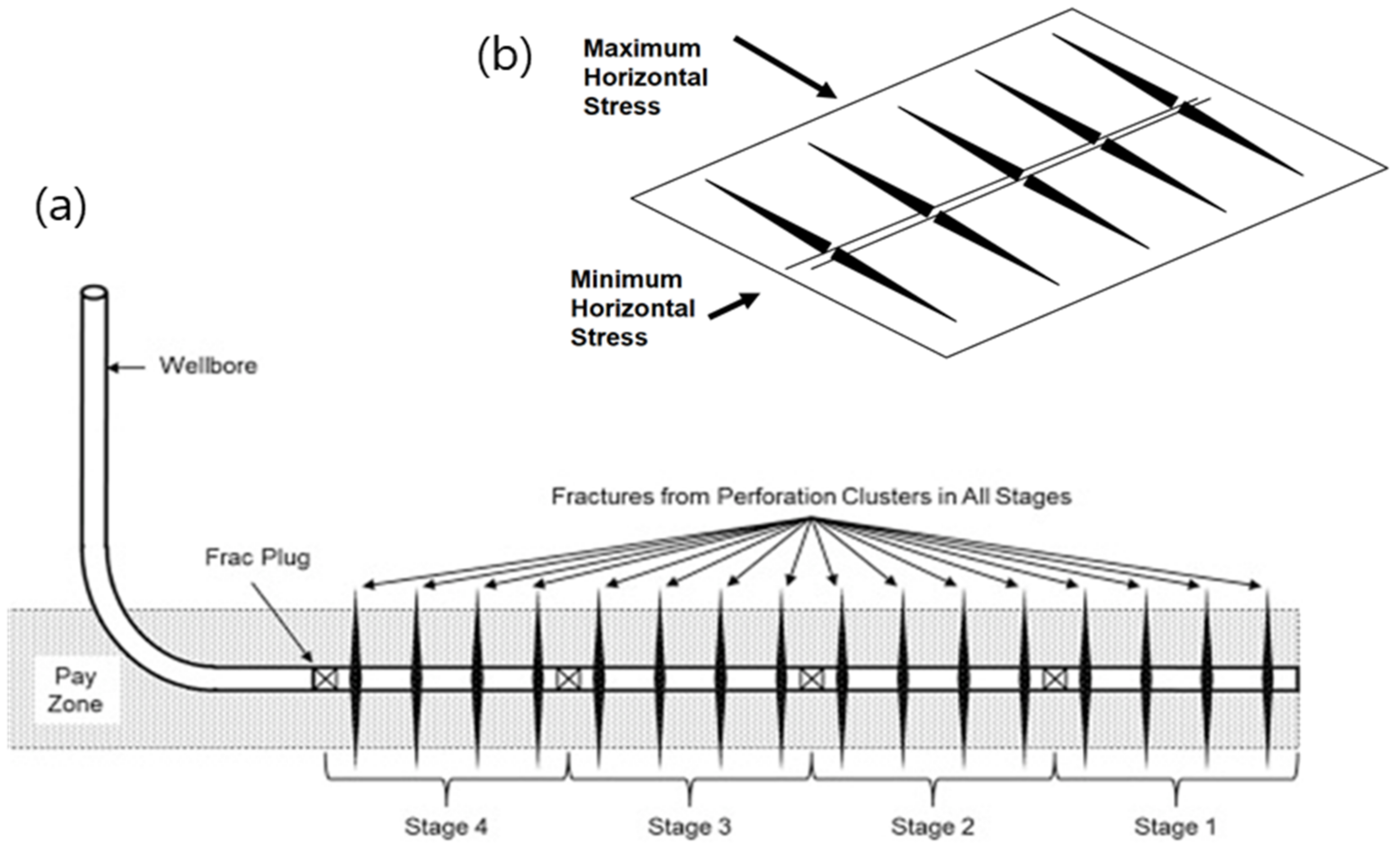
1]. Hydraulic fluid is pumped down from the wellhead into isolated sections (called fracture stages) of the wellbore that are pressure-isolated by frac plugs [
2], and the fractures are initiated from perforations of the wellbore placed in tight clusters at regular intervals (
Figure 1a). When the spacing distance between the perforation clusters is further reduced, down to ~3.3 m (10 ft) with the latest state-of-the-art well completion engineering technology, the intensity of mutual stress and strain interference between the individual hydraulic fractures increases [
3].
One of the more intriguing aspects of the stress redistribution process related to stress shadowing is that the minimum principal stress direction prior to the fracture treatment may become a maximum principal stress direction during the hydraulic fracture treatment (and vice versa). Such stress reversals have been reported by numerous authors [
4,
5,
6,
7,
8,
9]. Stress redistribution patterns and reversals vary greatly, depending on the native state of stress prior to fracturing, reservoir pressure waxing and waning during and after the fracture treatment, and the selected fracture spacing, as well as on whether fracture stimulation in the stages of adjacent wells occurs simultaneously, sequentially, or alternately [
10].
The consequence of stress shadows affects the growth and arrest of inner fractures in the treated stage more than the outer fractures, which may continue to grow, especially near the heel end of the wellbore [
11]. Theoretically, to avoid interference with the stress reversal zones of a prior fracture, the perforation spacing needs to be larger than the stress reversal zone width [
12]. Even with 183 m (600 ft) fracture spacing, stress reversals may still occur, with neutral stress points building between the fractures. Any new perforations near the midway position of the two prior fractures cannot grow fractures transversely; instead, the later fractures will curve toward one of the earlier, adjacent fractures [
10].
Zipper fracture treatment schedules were proposed to create more complex fracture networks [
13,
14], but these may be hampered by severe stress shadowing [
10]. When the fracture spacing is tightened, only outer fracs can propagate relatively unconstrained by stress shadows [
15,
16]. Narrower fracture spacing (<7.6 m (25 ft)) results in single fractures developing, because the outer fractures coalesce [
17].
As fracture treatment moves from the toe to the heel side of the well, the instantaneous shut-in pressure (ISIP) increases from one frac stage to the next [
18]. The net pressure required to achieve the same fracture half-length from each subsequent perforation cluster increases with each additional fracture created, as can be inferred from the ISIP escalation. Consequently, the stress reversal zones become wider with each additional consecutive fracture [
10,
19]. The closure stress ramps up quickly after the first couple of fracture stages, as captured in stress escalation type curves [
17]. Furthermore, simultaneous fracturing in the stages remains elusive, because fluid closer to the heel point of the well receives more hydraulic fluid due to viscous dissipation of flow toward the toe. Consequently, heel point fractures in a stage propagate faster, unless the perforation size is adjusted (reduced) to prevent heel bias.
Although the prior studies cited have drawn attention to the phenomenon of stress shadowing, until now, a simple systematic explanation for the mechanism of principal stress reversals has not been developed. This study shows, using a series of closed-form models based on the linear superposition method (LSM) first introduced by Weijermars et al. [
20], how systematic changes in the principal stress trajectory patterns occur. In addition, what has not been recognized before is that, in addition to the first generation of stress reversals occurring when the fracture treatment pressure is initially elevated, a second generation of stress reversals occurs during flow-back and production-related pressure depletion, as explained later in this study.
One important initial condition at the start of a fracture treatment operation is that the horizontal lateral of the well is commonly oriented in the direction of the least principal stress of the geological basin (
Figure 1b). Moreover, the maximum principal stress direction in the horizontal plane is assumed transverse to the well. These base-case orientations of the principal stresses are then subsequently modified when hydraulic fractures are placed transverse to the wellbore. All stress and strain visualizations in this paper show map views of the tensor fields around the vertical hydraulic fractures at the level of the model reservoir. Wellbores are not drawn but are consistently assumed to be present (as delivery means of the fracture treatment pressures) in a direction orthogonal to the hydraulic fractures. For example,
Figure 2c shows two simultaneous hydraulic fractures in a wellbore at
y = 0;
Figure 2d assumes two parallel wellbores, one at
x = −2 and one at
x = +2. Figure 3b also assumes two parallel wellbores, one at
x = −2 and one at
x = +2.
2. Methodology
This section explains the tools and methods used in the modeling approach. First, we explain the merits of the linear superposition method (
Section 2.1) and stress trajectory visualization (
Section 2.2). Then, we proceed, in the subsequent subsections (
Section 2.3,
Section 2.4,
Section 2.5 and
Section 2.6), to explain how to compute and conceptually treat the stress states and pressure changes associated with the various phases of fracture treatment intervention (fluid injection, leak-off, and flow-back) and production-induced pressure changes. Once those computational elements are in place, we proceed in
Section 3 to show—for each phase of pressure change—the effect on the principal stress trajectories, and how stress reversals occur due to the interaction of the deviatoric stresses and the changes in the reservoir pressure.
2.1. Linear Superposition Method (LSM)
The method of solution applied here is based on the linear superposition method (LSM) [
20]. For example, LSM can quantify the displacement field around multiple hydraulic fractures [
15], using transforms of the analytical expressions by Sneddon [
22] (see
Section 2.4). The resulting displacement field can be computed by simple vector field addition, and then a suitable constitutive equation can quantify the strain and stress contours for specific elastic properties involved. For example,
Figure 2a–d show the strain concentrations near the tips of a pair of fractures (transverse and parallel aligned) from a photo-elastic study (
Figure 2a,b) that were closely matched with analytical LSM solutions (
Figure 2b,c). The case of
Figure 2a,c applies to a single well in the
x-direction at
y = 0 with transversely placed hydraulic fractures in the
y-direction. The case of
Figure 2b,d applies to two parallel wells in the
y-direction at
x = −2 and
x = +2, each with single transverse fractures in stages that are mutually aligned.
Another example, first given here, focuses on the isochromatic fringe patterns visualized photo-elastically for a staggered pair of fractures (
Figure 3a) subject to a far-field stretch in a direction normal to the fracture planes, which is dynamically equivalent to the case of a pressured fracture [
23,
24]. The fringe pattern of
Figure 3a can be closely matched by an LSM solution (
Figure 3b), using the approach explained in Pham and Weijermars [
15]. The case of
Figure 3a,b applies to two wellbores in the
y-direction, one at
x = −2 and one at
x = +2, with staggered transverse fractures, such as those used in modified zipper fracking schedules [
16]. The full set of required equations is given later in the present paper.
2.2. Principal Stress Trajectories
A new step added to our code is the mapping of the principal stress trajectory patterns. Such trajectories are everywhere tangential—in each point of the studied elastic continuum containing the fractures—to the direction of the two principal stress axes.
The angles
and
refer to the positive angle between the
X-axis and the direction of each of the principal stress axes (
,
,
), while the required inputs,
,
, and
, for Equations (1a) and (1b), represent the magnitude of the stress tensor components in the 2D Cartesian solution space, as can be computed throughout the fractured medium using the expressions given in
Section 2.3 and
Section 2.4.
Examples of the stress trajectory patterns for each of the cases in
Figure 2a,b and
Figure 3 are given in
Figure 4a–c. The trajectories stay parallel and perpendicular to the pressurized fractures, as long as the fracture inner walls remain separated, such that no shear due to friction between the walls may occur. If a shear component appears in the LSM solution, such a local shear may be subtracted by applying an interval vortex corresponding to the amount of shear displacement that needs to be removed. No such correction was necessary in the stress trajectory examples of
Figure 4a–c.
The stress trajectory patterns around the pairs of hydraulic fractures, each loaded with the same internal fluid pressures (
Figure 4a–c), do not change when the magnitude of the pressures in the two fractures are either increased or decreased at the same rate. However, when individual fractures are loaded with different internal pressures, the stress trajectory patterns shift as can be visualized with LSM; however, this is of less interest for the present study because, at a certain depth in a fractured reservoir, all fractures are likely loaded by similar net pressures, which may indeed vary over time.
In the next subsections, we first explain how we compute, in the LSM models, (1) the initial reservoir pressure (
Section 2.3), (2) the pressure change during the fracture treatment (
Section 2.4), (3) the pressure change during leak-off and flow-back (
Section 2.5), and (4) production-induced pressure changes (
Section 2.6). Once those computational elements are in place, we proceed in
Section 3 to show—for each phase of pressure change—the effect on the principal stress trajectories, and how stress reversals occur due to the interaction of the deviatoric stresses and the changes in the reservoir pressure. It is important to understand from the outset that the fluid pressures in the hydraulic fractures and the reservoir pore space are scalar quantities, in contrast to the deviatoric stresses, which are tensor quantities that need to be computed by different means at each step of the analysis, as detailed below.
2.3. Computing Initial Stress State and Reservoir Pressure
Our analysis assumes a plane strain boundary condition, which essentially renders the solution space 2D, coinciding with a horizontal plane in the target zone (
Figure 2), whereas the state of stress is evaluated in 3D. The initial tectonic stress state in the reservoir in geomechanics literature is typically given as stress gradients,
, , and
, as summarized in
Table 1 for a typical Andersonian case of strike slip. By choosing the reference frame for Cartesian coordinates parallel to the principal native stresses (
,
, and
), their values near the hydraulically fractured wellbore (
Figure 5) follow from the product of the near-wellbore depth studied and each of the stress gradients as given in
Table 2. It is also practical to align the
Y-axis with the wellbore, as shown in
Figure 5.
The Sneddon solution, used as a starting point for modeling the state of stress around multiple hydraulic fractures [
15,
16], assumes a plane strain boundary condition (
). A constitutive equation for isotropic linear elasticity quantifies the strain response to the applied stress, which, for the 2D case of plane strain, reduces to just three relevant strain gradient tensor components:
The required input values for
and
in Equations (2a)–(2c) are given in
Table 1. The displacements in the
X-,
Y-, and
Z-directions of every point of the elastic continuum now follow from the 2D strain tensor elements [
26].
The initial reservoir pressure is commonly specified as a pressure gradient. If equal to the pressure of a native water column connected all the way up to the surface, the formation pressure, Pf, is given by the product of the hydrostatic gradient, , and depth, i.e., Pf = z. However, if the reservoir is sealed off from the surface by the overlying strata, the burial history and tectonic stress today cause volumetric deformation of the pore space, whose pressure component is included in the information derived from geotechnical wireline logs. The initial reservoir pressure may vary and is generally classified as normally pressured (Pf = z), over-pressured (z > Pf), or under-pressured (z < Pf).
2.4. Computing Impact of Fracture Treatment on Stress State and Reservoir Pressure
The pressure load on the hydraulic fractures is assumed equal to the minimum horizontal stress. The displacement field due to fracture treatment of
n fractures can be found using the Cartesian transform of the Sneddon equation [
15].
Direct inputs needed are, for each fracture
i, the hydraulic net pressure,
P0, the position vectors,
r,
r1, and
r2 for the center and tips of each fracture, and their orientations,
θ,
θ1, and
θ2 (see
Figure 6). The hydraulic net pressure,
P0, is the load on the hydraulic fractures due to the compressors injecting the frack fluid, net of the leak-off.
For a fracture centered at an arbitrary point,
P(
xs,
ys)—rather than at the origin—and a fracture half-length of
xf, the appropriate transformation of coordinates is as follows:
where (
xNEW,
yNEW) are in the new coordinate system used for all calculations. The following equations can be derived for
θ,
θ1,
θ2,
r,
r1, and
r2 (
Figure 6) to describe the polar angles of the intended fracture in Cartesian coordinates:
The atan function is the four-quadrant inverse tangent of its variables. This would mean that all θ, θ1, and θ2 are positive values.
The basic equations required to compute the elastic displacements associated with the native state of stress and the superposed elastic displacement field due to the pressure-loading by hydraulically pumping fluid into the three hydraulic fractures of interest are now specified. The initial reservoir pressure is not significantly or directly affected by the injected fluid pressure, but by the elastic response of the host rock creates stresses that can be computed from Sneddon-based displacement equations (Equations (4a) and (4b)). The total fracture treatment stresses have a deviatoric component and a pressure component. Translation of displacement gradients to stresses occurs via a constitutive equation, assuming linear elasticity (see Appendix A in [
20]).
2.5. Computing Impact of Leak-Off and Flow-Back on Stress State and Pressure Changes
The excess net pressure on the hydraulic fracture walls from the mixture of frack fluid and proppants pumped into the stage, typically over a period of 30 min, falls off almost immediately after the compressor stops pumping fluid. The positive pressure gradient of the hydraulic fracture system, during hydraulic-fluid injection, becomes—during flow-back of the injection fluid—a negative pressure gradient, as required to maintain flow toward the wellhead in the production system. Leak-off is then allowed to occur, while the subsequent stages are pumped with fluid down the liner of the well. After about 2 weeks, all stages in the well will have been completed, and a period of flowback commences in the well system. Note that flowback may only occur when the pressure gradient in the production system of the hydraulically fractured well flips from positive—during the treatment of the stages—to negative at the onset of flowback. The initial production rate also briefly flows faster than the rate that would have occurred due to the initial reservoir pressure, prior to the fracture treatment.
2.6. Computing Impact of Pressure Depletion during Production
The production of fluid from the reservoir lowers the initial reservoir pressure as controlled by the well system (choke setting, pump, and diameter of production tubing). The production-induced pressure changes in the reservoir can be computed from a reservoir simulator or analytical well testing expressions; alternatively, they can be empirically based on changes in the wellhead pressure measured by the production system.
3. Results
In this section, LSM model results are presented to explain and illustrate with principal stress trajectories how stress reversals occur due to the interaction of the deviatoric stresses and the changes in the reservoir pressure during the fracture treatment phases of (a) fluid injection (
Section 3.1), (b) leak-off and flow-back (
Section 3.2), and (c) production (
Section 3.3).
3.1. Fracture Treatment-Induced Stress Changes
In reservoirs, where the wells to be completed are not subject to any tectonic stress anisotropy prior to the fracture treatment operation, the state of stress—due to the injection of frac fluid—can be computed from the elastic displacement field Equations (4a) and (4b), adopting certain elastic constants. Examples of the pertinent stress trajectory patterns for such cases were given in
Figure 4a–c. However, if elastic displacements pre-exist in the reservoir, due to the presence of a native tectonic stress anisotropy (Equations (3a)–(3d)), then the pre-existing stress state will be overprinted by the elastic displacement field of the fracture treatment operation (Equations (4a) and (4b)). For such cases, diagnostic stress trajectory patterns will develop, from which the occurrence of stress reversals immediately becomes apparent.
Figure 7a shows a typical example of the initial uniform stress state, using the parameters of
Table 1. The stress trajectories form a rectangular grid, with the maximum principal stress in the horizontal direction parallel to the
x-axis. For hydraulic fracturing, the well would be drilled at
x = 0 in the
y-direction, which is the minimum horizontal stress direction in map view.
Figure 7b gives the pertinent stress trajectory pattern resulting from the fracture treatment around a single stage
with two transverse hydraulic fractures. We now see that the direction orthogonal to the hydraulic fractures is in compression (
Figure 7b), which is a stress reversal as compared to the local stress state prior to the fracture treatment (
Figure 7a). Outside the region occupied by the hydraulic fractures, the stress reverts to the original tension in the
y-direction. The stress reversal occurs in a so-called neutral point (
Figure 7b).
The position of the neutral points changes with the relative magnitudes of the stress anisotropy and the net pressure on the fractures. A so-called stress cage forms around the hydraulic fractures (
Figure 7c), similar to what has been documented extensively in prior studies for over-pressured wellbores [
27,
28,
29]. Inside the elliptical stress cage zone, the largest principal stresses (compressive, blue trajectories) are in orientations transverse to the hydraulic fractures, whose direction was previously aligned with the minimum principal stress direction of tension. The position of the neutral points and the size of the stress cage domain vary with the relative magnitude of the far-field stress and the pressure load of the hydraulic fractures. For boreholes, the migration pattern of the neutral points can be systematically mapped using two qualifying parameters, the Frac number and a biaxial stress factor [
28]. Here, we suffice with giving examples for an active injection case (
Figure 7c), which has a lower injection pressure than used in
Figure 7b. With the impact of the elastic displacements due to the fracture treatment in
Figure 7c being weaker than in
Figure 7b, the neutral points occur closer to the hydraulic fractures. The stress cage domain in
Figure 7c is smaller than that in
Figure 7b, which corresponds to what has been documented for boreholes in the studies cited.
Figure 7d gives a profile along the line through
y = 0 for the case of
Figure 7c, restricted to the positive part of the
Y-axis. The three neutral points, marked by red dots in
Figure 7c, correspond to the crossing points seen in
Figure 7d. In these points, only a pressure (and no stress anisotropy) exists.
3.2. Leak-Off- and Flow-Back-Induced Stress Changes
During the injection of hydraulic fluid (prior to flow-back), the pressure in the fracture is higher than the initial reservoir pressure. The excess (net) pressure is given by the difference between the fracture pressure and the initial reservoir pressure.
Figure 8a shows that the largest principal stresses (compressive, blue trajectories) that were initially parallel to the orientation of the hydraulic fracture quickly turn into a direction transverse to the hydraulic fracture during the fracture treatment. This is the first generation of stress reversals. The stress reversal region typically occurs confined to an elliptical domain around the hydraulic fracture (dashed red ellipse, though the two neutral points in
Figure 8a).
During leak-off, the pressure in the fracture treated stages rapidly drops. The onset of flow-back corresponds to a situation where the fluid pressure in the reservoir becomes higher than the fluid pressure in the hydraulic fractures. The difference between the initial reservoir pressure and the bottomhole pressure, in the well and its fracture system, now becomes negative. For example, assume an initial reservoir pressure of 30 MPa and a bottomhole pressure for a well on natural flow of 20 MPa; then, the initial net pressure in the well system would be close to −10 MPa. When the pressure gradient in the well system reverses from positive to negative, the flow-back period starts. The hydraulic fractures then close on the injected proppant packs.
Curiously, the profound impact of the pressure change on the elastic displacements near the hydraulic fractures during flow-back has not been emphasized before in any prior study. The prior elastic displacements, due to the injected fluid pressure rise relative to the initial reservoir pressure, will have been completely undone at flow-back time; instead, they will result in elastic displacements caused by a negative net pressure.
Figure 8b shows the stress trajectories for a flow-back case, with a net pressure of −20 MPa. We now see that the state of stress in the direction normal to the hydraulic fracture has given way, again, to extension, which is the second generation of stress reversals. The stress reversals caused by the elevated fluid pressure during the injection period (
Figure 8a) have been rapidly undone. This is, in fact, no surprise. Fiberoptic observations from fracture treatment stages in the field (see discussion, in
Section 4.3) confirm the occurrence of the stress regime reversals independently explained by LSM models in the present study.
The other important feature of
Figure 8b is the recognition of a so-called fracture cage, i.e., an elliptical domain around the hydraulic fractures where the stress trajectories are no longer conducive for letting any natural fractures, positioned transverse to the hydraulic fracture, propagate outside the fracture cage. The phenomenon of such fracture cages was previously documented to occur around under-pressured boreholes [
27,
28,
29,
30,
31,
32]. Detailed comparisons of the dynamics of stress cages and fracture cages, near boreholes and hydraulic fractures, respectively, are given in
Section 4.1.
3.3. Production-Induced Stress Changes
As production proceeds and the wells are placed on artificial lift, the elastic displacements caused by the negative net pressure in the production system steeply increase. For example, if the initial reservoir pressure is 30 MPa and the bottomhole pressure due to the pump is 10 MPa, the net pressure in the well system would be close to −20 MPa.
Figure 8b shows the stress trajectory pattern due to the imposed net pressure of −20 MPa. The state of stress around the hydraulic fractures has now intensified into a stronger compressive stress regime in the direction normal to the hydraulic fractures. The crushing forces on the proppant packs will steeply rise—due to the transition from natural flow to artificial lift—and may cause further reduction in the conductivity of the fracture system. Field observations of micro-seismic activity during the early years of production suggest that significant settling and shifts take place during the early years of production (for a discussion, see
Section 4.6).
6. Conclusions
The present analysis used a recently developed linear superposition method (LSM) to produce the following new insights:
Stress trajectories can be rapidly visualized with LSM.
Principal stress orientations near hydraulic fractures may wander over time.
We show that two generations of such stress reversals occur.
A first reversal occurs during the fracture treatment intervention.
A second reversal occurs during production due to pressure depletion.
This new insight is important for improving fracture treatment operations.
The detailed analysis focused on the reversal of the principal stress orientations that may occur near hydraulic fractures of well systems used for energy extraction. At least two generations of stress reversals occur around the hydraulic fractures: an early, short-lasting episode occurs on the day of fracture treatment; a second generation of long-lasting stress reversals commences immediately after the onset of so-called flow-back. During these stress swaps, reservoir directions that were previously in compression subsequently exhibit extension, and directions previously stretching subsequently exhibit shortening.
The pressure change in the hydraulic fractures—from over-pressured to under-pressured (only held open by proppant packs)—causes the neutral points that separate domains with different stress states to migrate from locations transverse to the fracture to locations beyond the fracture tips. Understanding such detailed geo-mechanical dynamics, related to the pressure evolution in energy reservoirs, is extremely important for improving both the fracture treatment and the well operation, as future hydrocarbon and geothermal energy extraction projects emerge.


