Abstract
The main equipment responsible for connection and transmission of electric power from generating centers to consumers are power transformers. This type of equipment is subject to various types of faults that can affect its components, in some cases also compromising its operation and, consequently, the electric power supply. Thus, in this paper, electromagnetic, thermal, and structural analysis of power transformers was carried out with the objective of providing the operator with information on the ideal moment for performing predictive maintenance, avoiding unplanned shutdowns. For this, computational simulations were performed using the finite element method (FEM) and, from that, the different transformer operation ways, nominal currents, inrush current, and short-circuit current were analyzed. In this perspective, analyses of the effects that thermal expansion, axial forces, and radial forces exerted were carried out, contributing to possible defects in this type of equipment. As a study object, simulations were carried out on a 50 MVA single-phase transformer. It is important to emphasize that the simulations were validated with real data of measurements and with results presented in the current literature.
1. Introduction
Considering the great importance of power transformers for energy transmission, several studies have been developed with a focus on the analysis and solution of problems that affect this equipment and put the power system reliability at risk. There are several factors that can generate failures in power transformers during their useful life, but this article will analyze the temperature rise and the deformation of the windings. The increase in the internal temperature in the windings is due to the losses that occur during the operation, most commonly caused by the Joule effect. The deformation of the windings is mostly caused by the action of the magnetic forces generated inside the transformer.
A major aggravating factor in transformer failures is the occurrence of transient phenomena. Among the many transient events that cause failures, those caused by inrush and short-circuit currents are responsible for the majority of operation interruptions in transformers. The magnitude of inrush current may be as high as 10 times or more of transformer-rated current, which can cause malfunction of protection system [1]. Short-circuit currents induce excessive forces in the transformer windings that result in deformities in the winding, affecting its mechanical and electrical characteristics [2]. They also impose several disturbances such as voltage drop, false disconnections of protection devices, and mechanical stresses in the transformer windings [3].
The correct distinction among the many types of faults is also essential for the correct operation of transformer protection systems. In Yazdani et al. [4], the authors developed an artificial intelligence-based algorithm of protection systems for distinguishing among the types of transformer faults. Bayesian classifiers and artificial neural networks are used in conjunction to discriminate the system’s current condition as normal, internal fault, magnetizing inrush currents, over-excitation, and current transformer saturation.
Power transformers are required to withstand short-circuit currents without suffering thermal or mechanical damage, and after the fault is eliminated, they must cool down back to normal temperature at rated load. The design of more fault-tolerant transformers is essential to meeting these goals. In Yazdani et al. [5], the authors designed, fabricated, and tested a monophase transformer with fault current limitation, extended withstand time, and improved recovery capabilities. Those improvements were obtained in part due to liquid nitrogen subcooling and the use of high-temperature superconducting (HTS) wires insulated with thermal insulating solid polymer. In Yazdani et al. [6] reports heat transfer measurements relevant to the design of HTS transformer windings. Among its findings, one can find that the subcooled liquid nitrogen significantly increased boiling heat transfer compared to saturated vapor pressure (SVP), and that for HTS windings, solid insulation presented better thermal properties compared to paper insulation. With the high and increasing values of capitalized loss in several power transformers, electric utility companies are continuously re-evaluating the cost/performance characteristics of their grid system, with special attention to transformer designs. In addition, thermal analysis plays an important role in these cases since the thermal behavior of the transformer is a key component in the analysis of life expectancy [7].
An alternative to minimize these costs is computational modeling through the finite element method (FEM), which can assist transformers manufacturers in their design phase without requiring the fabrication of prototypes. They can be used by manufacturers to find faults that can shorten the life of the electromagnetic device [8].
Several works within the scientific society effectively show how the FEM can be used to indicate points of improvement in transformers such in Zhang et al. [9], which presents investigations of short-circuit current, electromagnetic force, and transient dynamic response of winding deformation, including mechanical stress, deformation, and displacements for a 220 kV oil-immersed power transformer, considering the nonlinear elasticity characteristic of the spacers, the results of dynamic mechanical stress, and deformation induced by the combination of short-circuit and pre-force—efforts that are useful for the design of the transformer and fault diagnosis. In Zhao et al. [10], continuously transposed conductors (CTC) are analyzed, introducing a local asymmetry in the transformer windings, and the failure analysis shows that building an asymmetric structure in transformers increases the risk of deformation in these windings, with the results indicating that the transposition structure distorts the distribution of the magnetic field by increasing the maximum amplitude of the radial magnetic flux density in the transposition structure and that the initial stage of the elevation segment in height of the CTC is a weak point and should be strengthened in the process of manufacturing.
The use of FEM simulations is one of the best cost-effective alternatives to solve engineering problems. However, to obtain results increasingly closer to physical reality, simulations must consider the coupling between several physical phenomena (multiphysics), as demonstrated in Fonseca et al. and Yana et al. [11,12].
The use of numerical simulations via FEM to analyze different phenomena in transformers such as electromagnetic, thermal, structural, fluid, acoustic, and vibration, among others, is well established. For example, one can accurately estimate the dispersion of the magnetic field density in the transformer and find the values of the forces in the axial and radial directions that cause structural deformation in the windings [13]. In Wang et al. [14], the cumulative stress–strain characteristics of transformer windings were analyzed using a 3D FEM coupled electromagnetic structural analysis solution in a two-winding 110 kV transformer. From the results of the analysis, we verified that the characteristics of the material of the transformer winding and the state of tension can determine the shape of the winding deformation, as well as the type and the extent of the deformation.
The application of FEM makes it possible to analyze complex phenomena in an efficient way, such as in Gołebiowski et al. [15], where the losses due to eddy currents in laminated magnetic nuclei were analyzed. However, despite the fact that FEM presented fairly coherent results, it was necessary to couple different physical phenomena in order to more accurately represent what happened in the equipment, as well as in couplings such as electromagnetic-structural, electromagnetic-thermal, and thermal-fluid, among others.
Another form of coupling is presented in Zhang et al. [16], where a 500 kV 2D finite element elec-tromagnetic-mechanical coupling model was developed to analyze the transient failure process, considering the resistance–temperature relationship and plastic displacement in thermal systems and mechanical winding characteristics.
Several coupling methodologies are already being studied, such as the one presented in Wang et al. [17], a magneto-structural coupling for the short-circuit condition using finite elements, considering the nonlinear characteristics of the spacers in order to assess the distribution of magnetic forces over the windings and deformations generated using a 110 kV transformer as the object of study.
Another coupling methodology was used in Li et al. and Gong et al. [18,19] in order to evaluate the temperature distribution of the transformer winding, since local heating can accelerate the aging of insulating materials. In these works, a magneto-fluid-thermal coupling model was developed to calculate the temperature rise and predict the potential critical points of a simplified 2500 kVA dry-type power transformer and a 220 kV transformer.
In Zhang et al. [20], a method was developed to analyze the buckling resistance of transformer windings on the basis of the electromagnetic thermal structure coupling method. The influence of plastic deformation and the thermal effect on the final load of instability is considered in a three-phase dry type transformer, where thermal analysis was developed in 2D and the others in 3D.
Coupling methodologies also involve the interaction between different numerical methods in order to consolidate the results even more precisely, such as the coupling shown in Lima et al. [21], where the trapezoidal method coupled to the FEM was used to analyze the phenomenon of solidary energization in a three-phase bank formed by three single-phase transformers.
Most of the works involve only two physical domains, such as electromagnetic-thermal, electromagnetic-structural, thermal-fluid, and thermal-structural; the few works that currently combine three physical domains in computer simulations use in at least one of the stages the simulations in 2D. Unlike previous research, in this work, a coupling was made between three different physical domains, magnetic-thermal-structural, where in all stages 3D modeling was used for greater precision and detail of the results.
In this way, using a 50 MVA transformer as a study tool, we developed a 3D magnetic-thermal-structural analysis via FEM, considering the nominal current, the inrush current, and the short-circuit current to evaluate the heating and the mechanical deformation of the windings. All simulation results were compared with measurement data for validation of the methodology.
2. Materials and Methods
Before presenting the results obtained in this work and the scientific contributions, we present a synthesis of physical and numerical parameters used to develop this research, depicting some of the main equations used.
2.1. Finite Element Method
FEM is a numerical method used to solve complex problems by calculating the nodal energy potential. To apply such methodology, one must divide the complex problem into simpler subproblems (Figure 1); these simpler subproblems take the form of a geometrical element defined according to the problem to be studied—in the case of this research, the tetrahedral element.
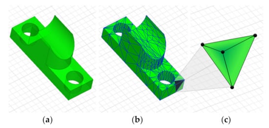
Figure 1.
Basic definition of the FEM: (a) complex geometric problem (b) discretization of the problem, (c) simple geometry (tetrahedric).
One of the main elements used for three-dimensional problems is the tetrahedral element; this element has four nodes, and the point calculation of the nodal potentials can be defined by (1).
From the Cartesian coordinates of the four nodes of each element, one can also calculate the potential according to (2), where D is the determinant of the matrix formed by the coordinates of the element [22].
For the derivation of the shape functions, using the tetrahedral elements, one must use volumetric coordinates, since to model 3D problems, the volume is a quantity to be taken into account; in this way, the Cartesian coordinates can be interpolated through the volume coordinates. To integrate any generic function f(x, y, z) over the entire tetrahedral element, be it in the electromagnetic, thermal, or structural domain, this integration is performed in the reference element according to (3) [23].
where are volume coordinates of the element, and is the Jacobian matrix needed for the transformation from the volumetric coordinate system to the Cartesian coordinate system.
2.2. Magnetic Modeling
The analysis of electromagnetic devices, as in the case of transformers, requires knowledge of electromagnetic phenomena in interior and in the region around the device [24]. To do this, Maxwell’s equations are used, which describe the relations between electromagnetic quantities, allowing for temporal and spatial analysis of these types of equipment.
To solve the problem addressed in this work, we applied the magnetic scalar potential to solve (4).
Equation (4) describes the Ampere‘s law in its stationary form and is one of the equations that represent the set of Maxwell equations, where presents the relation of the rotational of magnetic field with current density . Defining a potential , derived from the magnetic field , one can arrive at the following relationship [25]:
Substituting the magnetostatic equations and , where is magnetic flux density and is the magnetic permeability of the medium, into formula (5), we obtain
Applying the Galerkin method, we obtain the following relationship [26]:
where
The first integral on the right side of (8) corresponds to the boundary conditions of the problem. Calculating the terms for the discretized domain,
This way, the formulation for the problem of the magnetic scalar potential is defined.
2.3. Calculation of Losses in Transformer Windings
The total losses , which results in higher temperatures in transformers, are generated for two kinds of losses that occur during their operation: losses in iron and in copper . The total loss that occurs in a transformer can be defined from the sum of these distinct losses.
However, for the development of this work, only losses of copper , which occurs due to the joule effect, will be considered.
The heat flow static problems address by FEM are heat conduction problems. These problems are represented by a temperature gradient, G, and heat flux density, F [27]. The heat flux density must obey Gauss’ Law, which says that the heat flux out of any closed volume is equal to the heat generation within the volume; this law is represented in differential form as
where q represents volume heat generation.
Temperature gradient and heat flux density are also related to one another via the constitutive relationship:
where (k) is the thermal conductivity.
FEM allows for the variation of conductivity as an arbitrary function of temperature. Usually, the goal is to find the temperature, T, rather than the heat flux density or temperature gradient. Temperature is related to the temperature gradient by
Substituting (13) into Gauss’ Law and applying the constitutive relationship yields the second-order partial differential equation:
FEM solves (14) for temperature T over a user-defined domain with user-defined heat sources and boundary conditions.
As in this work the losses by joule effect is modeled as a function of the current density, J, the heat generation can be defined as follows [25]:
where is the electrical conductivity of the material, is the angular frequency, and the current density can be defined taking into account the magnetic vector potential A [28].
The eddy current loss is written in terms of the current density as
If A corresponds to the peak value of the vector potential, then the loss in a first order triangle will be
where is the current density, is the complex conjugate of the current density, is the electrical conductivity of the material, and is the determinant of the matrix formed by the coordinates of the element. Since A varies linearly over the element, then by (16) so does ; therefore [29],
Substituting into (18)
Solving the integral, we have
This way, it is possible to determine the losses as a function of current density in the coil of transformer.
2.4. Calculation of Electromagnetic Forces in Windings
In the structural model, the objective of this work is to analyze the forces acting on transformer windings, which at high values can critically deform the internal structure of windings. According to the electrodynamic theory, force density in a given volume of a transformer winding can be defined by the following equation [30,31].
where the magnetic force density is related to the current density and the magnetic flux of dispersion in the winding; however, the dispersion field decomposes into two components, one axial and one radial, at the lower and upper ends of the windings. Figure 2 illustrates this decomposition of the magnetic dispersion flow.
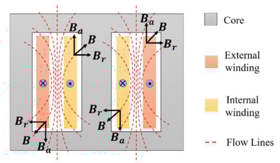
Figure 2.
Direction of the magnetic field in the windings by a transformer. Recreated from [31].
The previous equation can be decomposed into the following relations:
The axial force density is related to the radial magnetic flux , and the axial force density is related to the axial flux .
Radial forces are produced by the magnetic flux density of axial dispersion, presenting different behaviors for the external and internal windings. The value of the axial dispersion magnetic flux density increases from zero in the outermost region of the high voltage winding to a maximum value in the inner diameter (in the interval between the two windings). Therefore, the magnetic flux density of dispersion at the midpoint between the windings can be determined by (24) [32]
where is the magnetic flux density of axial dispersion, N is the number of turns in the winding, is the nominal current of the winding, is the height of the winding, and is the vacuum permeability.
Therefore, the radial force on a medium diameter winding can be determined by (25) as follows [32]:
where is the total radial force in the winding and is the average diameter in the winding.
As for the axial forces, the analytical calculations in a transformer with concentric windings are not simple or precise regarding the calculation of the magnetic flux density of radial dispersion. However, there are methods that provide approximate results, but the axial forces must be analyzed in two distinct ways, designated as ideal and non-ideal conditions [33].
In the ideal condition, the transformers have a uniform distribution of magnetomotive forces in concentric windings of equal length. For this condition, the sum of axial compression close to the midpoint for the external and internal windings can be obtained directly, according to (26) [34,35]
where is the magnetomotive force of the windings; is the average diameter of the transformer windings, considering the two windings; is the height of the windings; is the space between the windings; and and are the radial thicknesses of the external and internal windings, respectively.
For the non-ideal condition, there is a significant increase in axial force in these circumstances. Axial forces present greater complexity for the solution through analytical methods. This occurs mainly because of the difficulty in taking into account the curvature of the windings and the presence of the ferromagnetic core [34]. Thus, the density of the mean radial flow in the mean diameter of the transformer is given by (27).
where is effective length of the radial flow, is the conductor length, and is the nominal winding current.
The axial force on the other winding of the () maximum ampere-turns transformer can be determined by means of (28) [36]
The action of these forces on the windings in nominal operating conditions already exert a mechanical stress on the windings, and during the occurrence of a transient phenomenon, this stress worsens, further generating deformations in the windings.
The action of radial and axial forces causes different deformations in the windings. The axial force deforms the windings by compressing the upper and lower ends (Figure 3a). The radial force acts more intensely at half the height of the windings, expanding the outer winding and compressing the inner winding (Figure 3b).
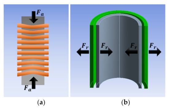
Figure 3.
Behavior of forces in the transformer winding: (a) axial, (b) radial.
The mathematical relationship to determine the deformation (in percentage of elongation) of a body in the elastic regime is obtained according to (29) [37].
where is the deformation suffered; is the elongation suffered; and are the final and initial lengths for the elongation, respectively.
3. Main Transients in Transformers
Transient phenomena may occur at various times during operation or during energizing of the transformers. These events are configured to raise the peak values of nominal currents in the machine to high levels. The main transients include short-circuit currents and inrush currents. Each phenomenon has specific effects, consequences, and durations as follows.
3.1. Inrush
The energizing current has a high initial peak value, as illustrated by Figure 4, and may exceed the peak current of rated current by as much as 20 times. Although this current typically appears during the energization of the transformer, other transients that occur in the circuit may cause this transient current to appear.
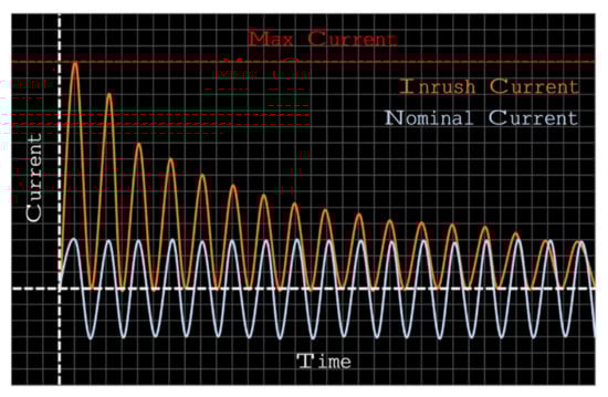
Figure 4.
Waveform characteristic of the inrush current.
Therefore, in order to mathematically determine the behavior of the inrush current as a function of time, one can use (30) [38,39]:
where is the maximum magnetic flux; is the residual flow; is the angle at the switching instant; is the number of turns of the winding; and and are the resistances and inductances of the primary winding, respectively.
However, there are other ways to calculate the peaks of the static inrush current, where the maximum peak is calculated and then coefficients are used to determine the decay of the waveform, in order to determine the current value of the first peak, as in (31):
where is the projected steady-state flux density value in the core, is the residual flux density, is the cross-sectional area of the core, is the mean area of a winding loop, and is the magnetic permeability of vacuum.
In this paper, only the first peak of the inrush condition was analyzed, which is the most critical case for transformers.
3.2. Short-Circuit
Short-circuit currents, besides being one of the most frequent causes of faults in transformers, are also among the faults that present greater severity in terms of impact on the structures of transformers support. Under the action of a short-circuit, the dispersion flux density increases significantly and, therefore, the forces acting on the windings also increase [30]. Figure 5 illustrates the characteristic curve of the short-circuit current.
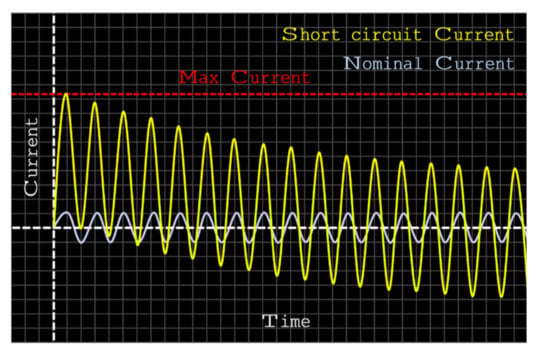
Figure 5.
Characteristic curve of the short-circuit current.
For simplification of empirical short-circuit calculations, the impedances of static components such as transmission lines, cables, reactors, and transformers are assumed to be time-invariant. Ignoring these effects and assuming that the transformer impedance () is time-invariant during a short-circuit, the transient and steady-state currents are given by the differential equation of the circuit with an applied sinusoidal voltage [40]:
where is the inductance, is the resistance, is the peak source voltage, is the angular frequency, is the frequency of the AC source, and is the angle on the voltage wave at which the fault occurs. The solution of this differential equation is given by
where is the maximum steady-state current, given by , and the angle . The transient current, given by the second term of (33), can be called a DC component and it decays at an exponential rate. Equation (33) can be simply written as
Although the short-circuit current presents this transient behavior, in this work, only the maximum current point of this phenomenon in a transformer will be analyzed; it can be calculated by (35) [26].
where is the asymmetry factor of short-circuit current, is the nominal power of the transformer in MVA, is the phase-to-phase nominal voltage of the transformer, and is the impedance of the transformer.
4. Results
The finite element method (FEM) has multiple applications; however, for the present paper, three different types of analysis coupling three different physical domains (magnetic, thermal, and structural) were carried out with three different modes of operation (nominal, inrush, and short-circuit) of a 50 MVA transformer. The simulations were developed using the Ansys Workbench commercial software, a computational tool widely used in academia to develop numerical FEM simulations. The analyses developed in this work are described in the following topics.
4.1. Transformer Data
The object of the study was a single-phase 50 MVA transformer connected to a three-phase bank that is in operation in Northern Brazil, as illustrated in Figure 6. Its factory characteristics are listed in Table 1.
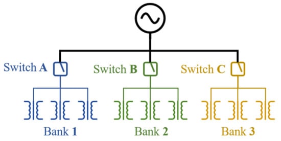
Figure 6.
Three-phase bench mounted by three single-phase transformers. Recreated from [21].

Table 1.
Characteristics of the 50 MVA transformer.
For the construction of the modeling of the transformer used in this work, we took into account the B-H curve of the ferromagnetic material, where the 1008 cylindrical steel was used, with a packing factor of 0.72. Copper was used to model the windings, in addition to following all the geometric parameters in Table 1.
From the transformer board data, we developed a computational model according to construction parameters. This model is shown in Figure 7.
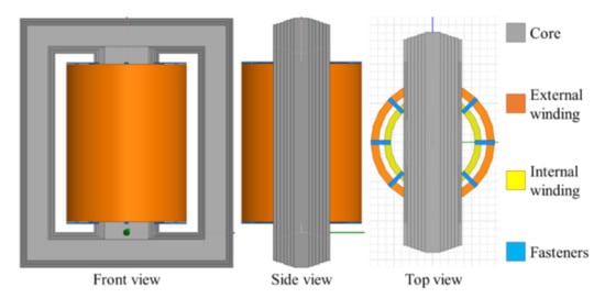
Figure 7.
Computational model of the transformer used in simulations.
4.2. Simulation in Nominal Operation
In the first moment, the modeling of the transformer under analysis was developed, and then the nominal operating current was inserted as a source of excitation for the electromagnetic analysis. After the solution of the electromagnetic equations, the losses by Joule effect were collected as results. These losses were inserted in a thermal simulation through a coupling, where it was possible to determine the temperature distribution along the transformer windings, as shown in Figure 8. Then, the temperature values obtained were compared with temperature values measured directly inside the transformer at the same time that the current values were collected to validate the developed thermo-magnetic coupling methodology.
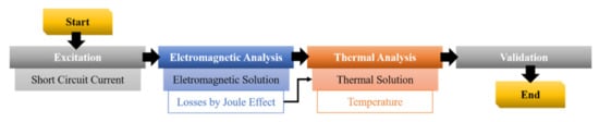
Figure 8.
Thermo-magnetic coupling.
As shown previously, the losses due to the Joule effect occur as a function of the current density, and thus this type of coupling is necessary to give more precision to the results since the losses are not evenly distributed along the transformer windings.
Considering that the main sources of heat in the transformers are the losses and the Joule effect, we initially performed magnetic simulations by inserting as input data the currents of 131.8 A in the external winding and 421.1 A in the internal winding; these current values were collected directly from the machine in operation.
Figure 9 shows the ohmic losses in the transformer windings from these results, and, using coupled simulations, the calculated losses were entered as a boundary condition for the thermal simulation.
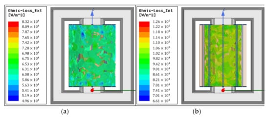
Figure 9.
Ohmic losses during nominal operation: (a) in external winding, (b) in internal winding.
After conducting the electromagnetic simulation for the nominal operating condition, we found that the losses in the internal winding (Figure 9b) were higher than the losses in the external winding (Figure 9a), thus describing what happens physically in the transformer.
In the sequence, the thermal simulation of the transformer was performed to estimate the temperature of the windings. Ohmic losses calculated in the electromagnetic simulation were inserted in the boundary condition as a heat source; copper emissivity of 0.018, ambient temperature of northern Brazil in the amount of 35 °C, and thermal conversion coefficient were also considered in the amount of 9 W/m2 °C.
In this way, it was possible to determine the temperatures of the transformer windings for the nominal operating condition, as shown in Figure 10.
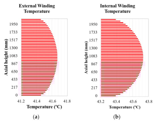
Figure 10.
Heat flow in the windings (a) in external winding, (b) in internal winding.
Analyzing the results of the thermal simulation, we were able to observe that the temperatures in the internal winding (Figure 10b) were higher than the temperatures in the external winding (Figure 10a); this was due to the fact that the losses in the internal winding were higher than the losses in the external winding.
In order to validate the computational methodology used in this work, we compared the data obtained with data collected directly from the equipment in nominal operation (Table 2).
Table 2.
Comparison of thermal data.
Table 2 shows the summary of the comparison between the thermal data. On the basis of this comparison, one can conclude that the methodology used for the simulations was valid, even having presented a significant margin of error between the values obtained in the simulation and the values measured by temperature sensors in the transformer.
When analyzing the data in Table 2, we were able to observe that the temperature values of the windings measured by sensors were higher than the temperature values found in the simulation. This was due to the fact that in the simulations developed in this work, oil temperatures and losses in the transformer core were not considered, whereas the transformer sensors captured the temperature of the transformer oil and used an analytical methodology to estimate the temperature of the windings.
4.3. Simulation with Inrush Current
In the second case, the same modeling of the transformer was used; however, in this case, the maximum peak value of the inrush current was applied as the energizing current for the electromagnetic simulation. After processing, the axial and radial forces generated in the external winding were collected as a result, as shown in Figure 11. Then, the calculated forces were inserted as a boundary condition in the structural simulation through the magneto-structural coupling, where it was possible to determine the radial deformation in the external winding. The deformation results found were compared with results found in the literature in order to validate the magneto-structural coupling methodology developed in this work.
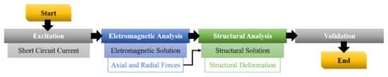
Figure 11.
Magneto-structural coupling.
Once the thermal part methodology was validated, simulations were performed, considering more severe operating conditions in order to analyze the deformation caused by the action of magnetic forces inside the machine.
Figure 12 shows the results obtained in magnetic simulation for inrush current operation, in which case a current of 1733.1 A was used in the external winding.
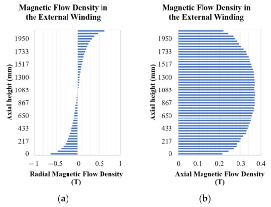
Figure 12.
Magnetic flux density: (a) radial, (b) axial.
From the axial and radial magnetic flux density, we were able to calculate the radial and axial forces, respectively. The calculated forces were entered as a boundary condition for the structural simulation in order to estimate winding deformation, as shown in Figure 13.
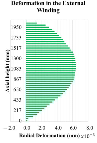
Figure 13.
Deformation of the external winding.
For the inrush condition, only the external winding was energized, and thus there was only the generation of electromagnetic forces in one of the windings.
Observing the results of the structural simulation, we obtained the value of mm as the maximum radial strain. The values found in this stage of the simulations were higher than the values found in the literature, as for example in Fonseca et al. [13], where a similar methodology was used with the same equipment under the same operating conditions. However, in Fonseca et al. [13], the electromagnetic stage was modeled in 2D, while in this work the electromagnetic part was modeled in 3D.
The difference between the results can be justified in Feng et al. [41], where the author compared simulation computational results in 2D and 3D and showed that, even with acceptable values, 3D simulations always present values higher than 2D results. This is because in 2D models, a simplification is used in geometries that present an axis of symmetry in addition to the use of a depth coefficient to approximate the model, whereas in 3D cases, the problem is fully modeled in the three dimensions.
Therefore, the methodology for the simulations can be considered valid.
4.4. Simulation with Short-Circuit Current
One of the main contributions developed in this article that is characterized by performing a 3D multiphysics analysis of a power transformer for the short-circuit condition coupling electromagnetic-thermal-structural phenomena. After validating the previous coupling methodologies, we built a new methodology based on the previous ones—however, in this case, using the maximum peak current of the short-circuit current as the excitation source.
Using the same modeling of the transformer shown above and inserting the short-circuit current as a source of excitation for the electromagnetic simulation, after processing, we extracted the Joule losses and axial and radial forces as results. In the sequence, the losses calculated in the electromagnetic analysis were inserted in the thermal simulation as a boundary condition, where it was possible to determine the temperature distribution along the windings of the transformer, and it was also possible to determine the thermal expansion suffered by the windings due to the high temperatures. Finally, a structural analysis was coupled to the set where the axial and radial forces calculated in the electromagnetic analysis and the thermal expansion calculated in the thermal analysis were inserted as a boundary condition. In this way, it was possible to reach a more precise structural deformation of the windings to the transformer since these consider electromagnetic and thermal elements that directly influence the structure of the transformer. The developed scheme for coupling the electromagnetic, thermal, and structural physical domains is illustrated in Figure 14.
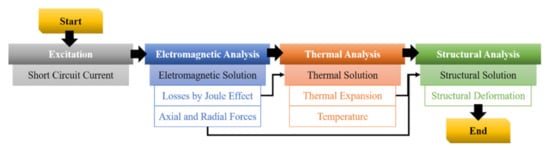
Figure 14.
Magneto-thermo-structural coupling.
As the last condition for the simulations of this work, short-circuit currents were adopted, a requirement that is considered to be one of the most severe among transients. Under these conditions, currents with amplitudes of 8979 A were adopted in the external winding and 34,586 A in the internal winding, where the following results were obtained.
Like the previous step, in the electromagnetic simulation, the current density was calculated in windings during the maximum peak of a short-circuit; due to Joule losses, these high-current values flowing through a conductor cause extreme heating inside the equipment, as shown in Figure 15.
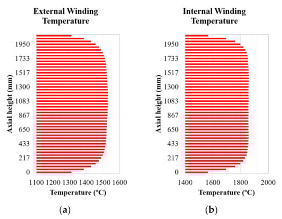
Figure 15.
Temperatures inside the transformer during a short-circuit (a) in external winding, (b) in internal winding.
Analyzing the temperature shown in Figure 15, we were able to see how critical a short-circuit is to a transformer, reaching temperatures that can break insulation or even melt winding discs. At this point, it is important to note that the current protection system should quickly isolate the fault, preventing the equipment’s temperature from reaching these extremely high levels. In this paper, this protection was not considered exactly for demonstrating the temperature level that can be reached if the protection system fails, which would certainly lead the transformer to irreparable damage.
In addition to current density, the magnetic simulations provide the determination of magnetic forces generated inside the transformer during short-circuit. From the magnetic forces and using coupled simulations, we determined the deformation suffered due to the interaction of magnetic forces and thermal expansion due to the heating. The joint action of all these factors resulted in the deformation illustrated in Figure 16.
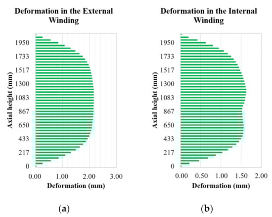
Figure 16.
Total deformation due to the action of magnetic forces and thermal expansion (a) in external winding, (b) in internal winding.
According to Figure 16, it is possible to observe that the deformation was more critical in the external winding; considering that the two previous conditions were validated, the results obtained in this step can be considered valid. Although the maximum deformation achieved reached 2.15 mm, this would already be enough to break the insulation and drastically compromise the operation of the transformer.
5. Conclusions
In this work, several analyses were developed combining electromagnetic, thermal, and structural phenomena using the FEM to analyze the behavior of a 50 MVA transformer operating with nominal current, inrush current, and short-circuit current.
- Initially the transformer was simulated using a thermo-magnetic methodology and considering the nominal operating current. The results obtained were compared with values measured by sensors to validate the methodology.
- In the second case, a magneto-structural methodology was used to simulate the same equipment; however, in this case, the maximum peak of the inrush current was considered as a source of excitation. Even though the results obtained in this step were higher than the results found in the literature, this difference is perfectly justified in view of the way in which this methodology was constructed.
- In the last step of the methodology of this work, a magneto-thermo-structural methodology was developed where the 50 MVA transformer was simulated considering the maximum peak of the short-circuit current as an operating condition. In this case, it was considered the most severe case that can occur in the transformers. The results found showed internal temperatures that can melt the contours, in addition to deformations that can easily break the insulation of the turns to the transformer.
- The methodology used in this work is very promising and the results obtained describe a projection for the physical behavior of the transformer; however, there are still points to be improved in future works, such as the use of this coupling methodology in transient analyses considering the operation curves, as well as the variation of the phenomena over time.
Author Contributions
Conceptualization, A.R.M.d.S., M.V.A.N., W.d.S.F., R.C.F.A., and D.d.S.L.; methodology, A.R.M.d.S., M.V.A.N., W.d.S.F., and D.d.S.L.; software, A.R.M.d.S., W.d.S.F., and D.d.S.L.; validation, A.R.M.d.S., M.V.A.N., and W.d.S.F.; formal analysis, A.R.M.d.S., M.V.A.N., W.d.S.F., R.C.F.A., and D.d.S.L.; investigation, A.R.M.d.S., M.V.A.N., W.d.S.F., and D.d.S.L.; resources, A.R.M.d.S., M.V.A.N., W.d.S.F., R.C.F.A., and D.d.S.L.; data curation, A.R.M.d.S., M.V.A.N., W.d.S.F., R.C.F.A., and D.d.S.L.; writing—original draft preparation, A.R.M.d.S., M.V.A.N., and W.d.S.F.; writing—review and editing, A.R.M.d.S., M.V.A.N., W.d.S.F., R.C.F.A., and D.d.S.L.; visualization, A.R.M.d.S., M.V.A.N., W.d.S.F., R.C.F.A., and D.d.S.L.; supervision, M.V.A.N., W.d.S.F., and D.d.S.L.; project administration, M.V.A.N. and W.d.S.F.; funding acquisition, A.R.M.d.S., M.V.A.N., W.d.S.F., R.C.F.A., and D.d.S.L. All authors have read and agreed to the published version of the manuscript.
Funding
This research was funded by the Pro-Rectory of Research and Post-Graduate Studies-PROPESP/UFPA.
Institutional Review Board Statement
Not applicable.
Informed Consent Statement
Not applicable.
Conflicts of Interest
The authors declare no conflict of interest.
Nomenclature
| FEM | Finite element method |
| HTS | High-temperature superconducting |
| SVP | Saturated vapor pressure |
| CTC | Continuously transposed conductors |
References
- Jamali, M.; Mirzaie, M.; Gholamian, S.A.; Cherati, S.M. A Wavelet-Based Technique for Discrimination of Inrush Currents from Faults in Transformers Coupled with Finite Element Method. In Proceedings of the 2011 IEEE Applied Power Electronics Colloquium (IAPEC), Johor Bahru, Malaysia, 18–19 April 2011; pp. 138–142. [Google Scholar]
- Sathya, M.A.; Thomas, A.J.; Usa, S. Prediction of Transformer Winding Displacement from Frequency Response Characteristics. In Proceedings of the IEEE 1st International Conference on Condition Assessment Techniques in Electrical Systems, Kolkata, India, 6–8 December 2013; pp. 303–307. [Google Scholar]
- León, F.F.; Jazebi, S. Analysis, Modeling, and Simulation of the Phase-Hop Condition in Transformers: The Largest Inrush Currents. IEEE Trans. Power Deliv. 2014, 29, 1918–1926. [Google Scholar]
- Yazdani-Asrami, M.; Taghipour-Gorjikolaie, M.; Razavi, S.M.; Gholamian, S.A. A novel intelligent protection system for power transformers considering possible electrical faults, inrush current, CT saturation and over-excitation. Int. J. Electr. Power Energy Syst. 2015, 64, 1129–1140. [Google Scholar] [CrossRef]
- Yazdani-Asrami, M.; Staines, M.; Sidorov, G.; Davies, M.; Bailey, J.; Allpress, N.; Glasson, N.; Gholamian, S.A. Fault current limiting HTS transformer with extended fault withstand time. Supercond. Sci. Technol. 2019, 32, 035006. [Google Scholar] [CrossRef]
- Yazdani-Asrami, M.; Staines, M.; Sidorov, G.; Eicher, A. Heat transfer and recovery performance enhancement of metal and superconducting tapes under high current pulses for improving fault current-limiting behavior of HTS transformers. Supercond. Sci. Technol. 2020, 33, 095014. [Google Scholar] [CrossRef]
- Daneshmand, S.V.; Heydari, H. Multiphysics Approach in HTS Transformers with Different Winding Schemes. IEEE Trans. Appl. Supercond. 2014, 24, 103–110. [Google Scholar] [CrossRef]
- Arjona, M.A.; Hernandez, C.; Escarela-Perez, R.; Melgoza, E. Thermal Analysis of a Dry-Type Distribution Power Transformer Using FEA. In Proceedings of the 2014 International Conference on Electrical Machines (ICEM), Berlin, Germany, 2–5 September 2014; pp. 2270–2274. [Google Scholar]
- Zhang, H.; Yang, B.; Xu, W.; Wang, S.; Wang, G.; Huangfu, Y.; Zhang, J. Dynamic Deformation Analysis of Power Transformer Windings in Short-Circuit Fault by FEM. IEEE Trans. Appl. Supercond. 2014. [Google Scholar] [CrossRef]
- Zhao, Y.; Chen, W.; Jin, M.; Wen, T.; Xue, J.; Zhang, Q.; Chen, M. Short-Circuit Electromagnetic Force Distribution Characteristics in Transformer Winding Transposition Structures. IEEE Trans. Magn. 2020. [Google Scholar] [CrossRef]
- Fonseca, W.S.; Lima, D.S.; Lima, A.K.F.; Soeiro, N.S.; Nunes, M.V.A. Analysis of electromagnetic-mechanical stresses on the winding of a transformer under inrush currents conditions. Int. J. Appl. Electromagn. Mech. 2016, 50, 511–524. [Google Scholar] [CrossRef]
- Yana, C.; Hao, Z.; Zhang, S.; Zhang, B.; Zheng, T.; Li, Z. Computation and analysis of power transformer winding damage due to short circuit fault based on 3-D finite element method. Int. J. Appl. Electromagn. Mech. 2016, 51, 405–418. [Google Scholar] [CrossRef]
- Fonseca, W.S.; Lima, D.S.; Lima, A.K.F.; Nunes, M.V.A.; Bezerra, U.H.; Soeiro, N.S. Analysis of Structural Behavior of Transformer’s Winding Under Inrush Current Conditions. IEEE Trans. Ind. Appl. 2018, 54, 2285–2294. [Google Scholar] [CrossRef]
- Wang, S.; Zhang, H.; Wang, S.; Li, H.; Yuan, D. Cumulative Deformation Analysis for Transformer Winding Under Short-Circuit Fault Using Magnetic—Structural Coupling Model. IEEE Trans. Appl. Supercond. 2016. [Google Scholar] [CrossRef]
- Gołebiowski, M.; Gołebiowski, L.; Smolen, A.; Mazur, D. Direct Consideration of Eddy Current Losses in Laminated Magnetic Cores in Finite Element Method (FEM) Calculations Using the Laplace Transform. Energies 2020, 13, 1174. [Google Scholar] [CrossRef]
- Zhang, B.; Lu, P.; Kong, J.; Liu, R.; Cao, Q.; Shao, H.; Deng, W.; Chen, J. Fault analysis and simulation of ground-fault accident on transformer in 500 kV AC/DC grids. Int. J. Appl. Electromagn. Mech. 2019, 60, 1–12. [Google Scholar] [CrossRef]
- Wang, S.; Wang, S.; Zhang, N.; Yuan, D.; Qiu, H. Calculation and Analysis of Mechanical Characteristics of Transformer Windings under Short-Circuit Condition. IEEE Trans. Magn. 2019, 55. [Google Scholar] [CrossRef]
- Li, Y.; Yan, X.; Wang, C.; Yang, Q.; Zhang, C. Eddy Current Loss Effect in Foil Winding of Transformer Based on Magneto-Fluid-Thermal Simulation. IEEE Trans. Magn. 2019, 55. [Google Scholar] [CrossRef]
- Gong, R.; Ruan, J.; Chen, J.; Quan, Y.; Wang, J.; Jin, S. A 3-D Coupled Magneto-Fluid-Thermal Analysis of a 220 kV Three-Phase Three-Limb Transformer under DC Bias. Energies 2017, 10, 422. [Google Scholar] [CrossRef]
- Zhang, B.; Yan, N.; Ma, S.; Wang, H. Buckling Strength Analysis of Transformer Windings Based on Electromagnetic Thermal Structural Coupling Method. IEEE Trans. Appl. Supercond. 2019, 29, 2. [Google Scholar] [CrossRef]
- Lima, D.S.; Mahmud, L.S.; de Sousa, A.R.M.; Fonseca, W.S.; Bezerra, U.H.; Bezerra, F.V.V. Electromagnetic analysis of single-phase transformer banks under sympathetic inrush phenomenon. Int. J. Appl. Electromagn. Mech. 2020, 62, 541–556. [Google Scholar] [CrossRef]
- Hollauer, C. Modeling of Thermal Oxidation and Stress Effects. Ph.D. Thesis, Technische Universität Wien, Vienna, Austria, 2007. [Google Scholar]
- Dias, F.; Cruz, J.; Valente, R.; Sousa, R. Método dos Elementos Finitos: Técnicas de Simulação Numérica em Engenharia, 2nd ed.; ETEP-Edições Técnicas e Profissionais: Lisbon, Portugal, 2018. (In Portuguese) [Google Scholar]
- Ebrahimi, B.; Fereidunian, A.; Saffari, S.; Faiz, J. Analytical estimation of short circuit axial and radial forces on power transformers windings. IET Gener. Transm. Distrib. 2014, 8, 250–260. [Google Scholar] [CrossRef]
- Bastos, J.P.A. Eletromagnetismo e Cálculo de Campos, 3rd ed.; Editora da UFSC: Florianópolis, Brazil, 1996; 452p. (In Portuguese) [Google Scholar]
- Bastos, J.P.A.; Sadowski, N. Electromagnetic Modeling by Finite Element Methods; Marcel Dekker Inc.: New York, NY, USA, 2003. [Google Scholar]
- Meeker, D. Finite Element Method Magnetics; User’s Manual, Version 4.2; [Online]; Available online: http://femm.foster-miller.net (accessed on 16 May 2020).
- Bianchi, N. Electrical Machine Analysis Using Finite Elements: Basic Principles of Finite Element Methods; Taylor & Francis Group: New York, NY, USA, 2005. [Google Scholar]
- Salon, S.J. Finite Element Analysis of Electrical Machines; Rensselaer Polytechnic Institute: Troy, NY, USA, 1995. [Google Scholar]
- Zhang, B.; Yan, N. Stability Analysis of Inner Windings in Transformers Based on Electromagnetic-Thermal-Structural Coupling Method 2p. In Proceedings of the IEEE International Conference on Applied Superconductivity and Electromagnetic Devices, Tianjin, China, 15–18 April 2018. [Google Scholar]
- Ahn, H.; Oh, Y.; Kim, J.; Song, J.; Hahn, S. Experimental Verification and Finite Element Analysis of Short-Circuit Electromagnetic Force for Dry-Type Transformer 4. IEEE Trans. Magn. 2012, 48, 819–822. [Google Scholar] [CrossRef]
- Kulkarni, S.V.; Khaparde, S.A. Transformer Engineering: Design and Practice; Marcel Dekker, Inc.: New York, NY, USA, 2012. [Google Scholar]
- Heathcote, M. J&P Transformer Book, 12th ed.; Oxford, Elsevier Science Ltd.: Madras, India, 1998. [Google Scholar]
- Waters, M. The Short-Circuit Strength of Power Transformers; McDonald & Co. Ltd.: London, UK, 1966. [Google Scholar]
- Fonseca, W.S. Análise de Esforços Eletromagneto-mecânicos nos Enrolamentos de um Transformador sob Condições de Correntes de Inrush. Ph.D. Thesis, Electrical Engineering Graduate Program. Federal University of Pará, Belém, Brazil, 2016. (In Portuguese). [Google Scholar]
- Azevedo, A.C. Estresse Eletromecânico em Transformadores causado por Curtos- Circuitos “Passantes” e Correntes de Energização. Ph.D. Thesis, Electrical Engineering Graduate Program. Federal University of Uberlândia, Uberlândia, Brazil, 2007. [Google Scholar]
- Hibbeler, R.C. Strength of Materials, 5th ed.; Tech. Sci. Books Publ.: São Paulo, Brazil, 2006. [Google Scholar]
- Kulkarni, S.V.; Khaparde, S.A. Transformer Engineering: Design, Technology, and Diagnostics, 2nd ed.; Marcel Dekker: New York, NY, USA, 2013. [Google Scholar]
- Faiz, J.; Ebrahimi, B.; Noori, T. Three- and Two-Dimensional Finite-Element Computation of Inrush Current and Short-Circuit Electromagnetic Forces on Windings of a Three-Phase Core-Type Power Transformer. IEEE Trans. Magn. 2008, 44, 590–597. [Google Scholar] [CrossRef]
- Das, J.C. Power System Analysis: Short-Circuit Load Flow and Harmonics; Amec, Inc.: Atlanta, GA, USA, 2002. [Google Scholar]
- Feng, J.Q.; Ma, C.; Tang, W.H.; Smith, J.S.; Wu, Q.H. A transformer predictive maintenance system based on agent-oriented programming. In Proceedings of the 2005 IEEE/PES Transmission and Distribution Conference & Exhibition: Asia and Pacific, Dalian, China, 5 December 2005. [Google Scholar]
Publisher’s Note: MDPI stays neutral with regard to jurisdictional claims in published maps and institutional affiliations. |
© 2021 by the authors. Licensee MDPI, Basel, Switzerland. This article is an open access article distributed under the terms and conditions of the Creative Commons Attribution (CC BY) license (https://creativecommons.org/licenses/by/4.0/).