Article

Study on Inelastic Strain-Based Seismic Fragility Analysis for Nuclear Metal Components

1
Korea Atomic Energy Research Institute, Daejeon 34057, Korea
2
Department of Civil and Environmental Engineering, Hanbat National University, Daejeon 34158, Korea
3
KHNP Central Research Institute, Daejeon 305-353, Korea
*
Author to whom correspondence should be addressed.
Energies 2021, 14(11), 3269; https://doi.org/10.3390/en14113269
Submission received: 25 March 2021 / Revised: 1 June 2021 / Accepted: 1 June 2021 / Published: 3 June 2021
(This article belongs to the Section H: Geo-Energy)

Abstract

:
The main purpose of this study is to investigate the feasibility of the seismic fragility analysis (FA) with the strain-based failure modes for the nuclear metal components retaining pressure boundary. Through this study, it is expected that we can find analytical ways to enhance the high confidence of low probability of failure (HCLPF) capacity potentially contained in the conservative seismic design criteria required for the nuclear metal components. Another goal is to investigate the feasibility of the seismic FA to be used as an alternative seismic design rule for beyond-design-basis earthquakes. To do this, the general procedures of the seismic FA using the inelastic seismic analysis for the nuclear metal components are investigated. Their procedures are described in detail by the exampled calculations for the surge line nozzles connecting hot leg piping and the pressurizer, known as one of the seismic fragile components in NSSS (Nuclear Steam Supply System). To define the seismic failure modes for the seismic FA, the seismic strain-based design criteria, with two seismic acceptance criteria against the ductile fracture failure mode and fatigue-induced failure mode, are used in order to reduce the conservatism contained in the conventional stress-based seismic design criteria. In the exampled calculation of the inelastic seismic strain response beyond an elastic regime, precise inelastic seismic analyses with Chaboche’s kinematic and Voce isotropic hardening material models are used. From the results of the seismic FA by the probabilistic approach for the exampled target component, it is confirmed that the approach of the strain-based seismic FA can extract the maximum seismic capacity of the nuclear metal components with more accurate inelastic seismic analysis minimizing the number of variables for the components.

1. Introduction

Recently, there have been many efforts to develop advanced seismic design rules that enable accommodating the increasing of the design-basis earthquake (i.e., SSE: Safe Shutdown Earthquake) for the nuclear facility components, especially for piping systems [1,2,3,4]. Furthermore, it is also true that there is a growing social demand that the beyond-design-basis earthquake must be considered in the design of the NPPs (Nuclear Power Plants) [5]. However, it is not easy to accomplish these needs under the current nuclear component design criteria based on the stress acceptance criteria [6], which have a conservative safety margin.
To assure the seismic integrity of the nuclear metal components, the seismic fragility analysis (FA) with a probabilistic method can be a candidate approach as an alternative seismic design rule for intentionally increased design-basis or beyond-design-basis earthquakes. Recently the seismic fragility analysis for the nuclear power plant structure and piping has been studied [7,8,9] and for various industrial structures [10,11], but the research for the nuclear metal components retaining high-pressure boundary is very scarce up to now. In actuality, the full seismic probabilistic risk assessment (SPRA) is required to prevent the potential risks of earthquakes in the NPPs [12,13,14,15]. This SPRA is composed of the four steps to be performed with (1) seismic hazard analysis, (2) component fragility analysis, (3) plant system and accident-sequence analysis, and (4) consequence analysis. Among them, only the component fragility analysis just for the seismic events is investigated in this paper in order to develop the benefit ways to estimate the maximum seismic capacity by the probabilistic approach.
In actuality, it is true that there are many general procedures and standards for a seismic FA but most detailed seismic FA procedures are different from case-by-case [15]. Currently, there are very few detailed specific procedures for the pressure retaining nuclear safety-related components.
The main purpose of this study is to establish the practical procedures of the seismic FA based on the previous study of the strain-based seismic design method applicable for the nuclear metal components retaining the pressure boundary, which have to be designed by the nuclear codes and standards. In actuality, there are some examples of the seismic FA developed for building shear wall, liquid storage tanks, heat exchanger, expansion anchor, and so on [15]. However, when we try to use the well-known standards, there are few studies to be able to refer practical procedures of the seismic FA for the nuclear pressure retaining components, which have to be complied with the rules of the nuclear codes and standards. Additionally, current failure modes considered in the nuclear codes and standards for the safety-related metal components are conservatively based on the stress limits. This paper is trying to establish more detailed practical procedures with the strain-based seismic failure modes for the seismic FA.
In performing a seismic FA, one of the important works is defining the failure modes. In general, the failure modes required for the seismic FA are defined to be the actual failure completely losing their load resistance or safety functions. However, in the case of the safety-related pressure-retaining nuclear metal components, the seismic failure modes should be compliance with the Level D Service Limits, such as the limits for general primary membrane stress against a failure by plastic instability or necking, and the limits for local primary membrane plus bending stress against a failure by collapse [16], which have a conservative safety margin. However, when the earthquake level is high enough to invoke near yield conditions or exceed the elastic limits on metal components, the failure modes will actually be controlled by the strain conditions rather than the stress conditions. To overcome the conservatism implemented in the current stress-based design criteria, the strain-based seismic design criteria are in development in many countries as an alternative rule for the nuclear metal components [3,4].
In this paper, the general procedures of seismic FA with the probabilistic approach are investigated with the previously developed strain-based seismic design criteria [17] for the nuclear metal components retaining high-pressure boundary, which inevitably require an inelastic seismic time history analysis. The procedures for performing fragility calculations of the high confidence of low probability of failure (HCLPF) capacity are based on the recommendations in the EPRI technical reports [15,18].
To validate the detailed procedures for HCLPF capacity calculations, example calculations for the surge line nozzles connecting hot leg piping and the pressurizer, known as one of the seismic fragile components in NSSS (Nuclear Steam Supply System), are performed. Such calculations follow the basic FA variables generically recommended in EPRI/TR-103959 [15].

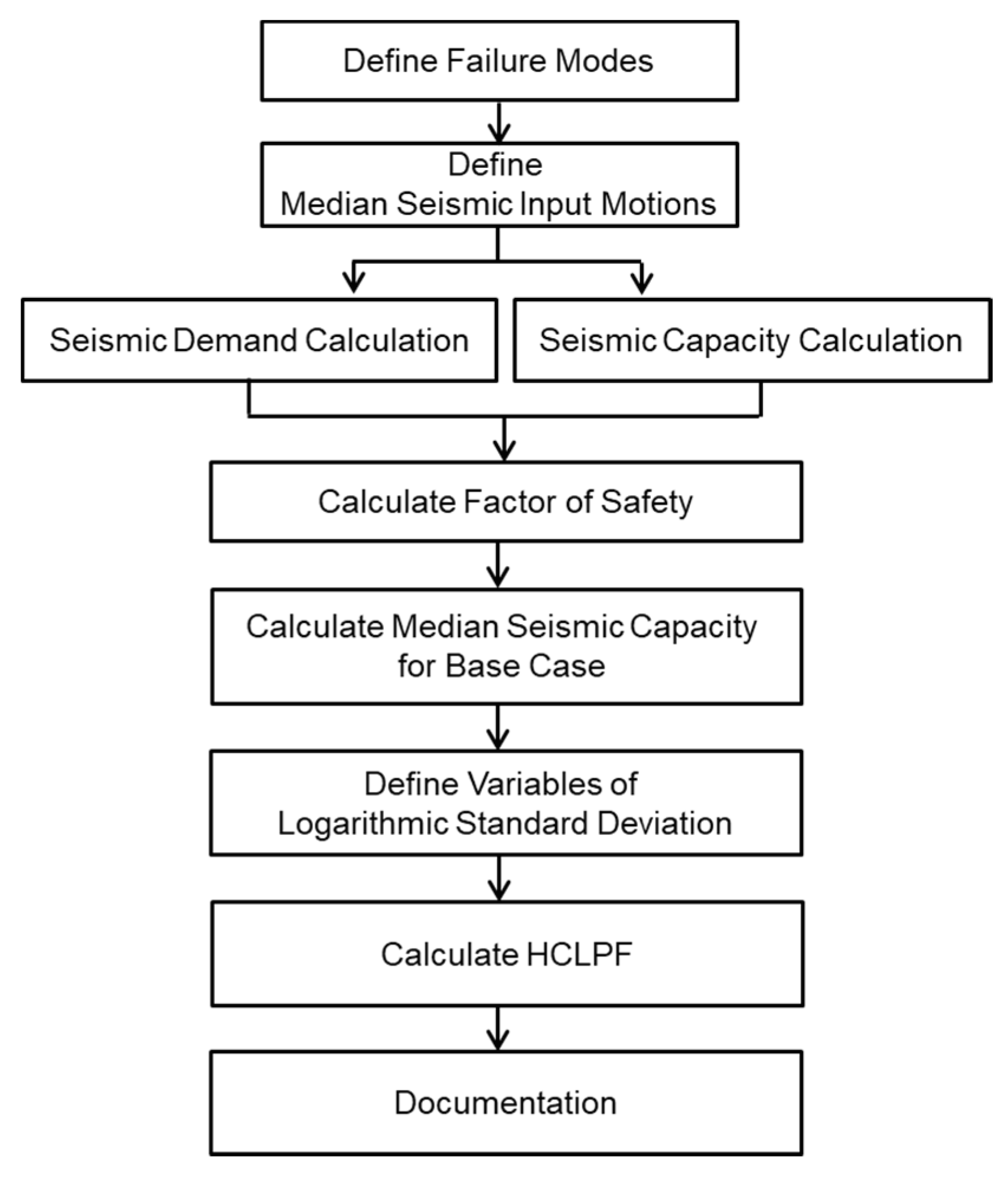
2. Procedures of Seismic FA for Nuclear Metal Components

This paper presents the overall procedure of the inelastic analysis-based seismic FA for the safety-related nuclear components. The final goal of the seismic FA is scoped to calculate the seismic HCLPF capacity, which probabilistically represents the seismic margin of components.
Figure 1 presents the main procedures of the seismic FA investigated in this study. The detailed approach for each procedure is described step by step and discussed as follows;

2.1. Definitions of Failure Modes

First of all, it is essential to define the seismic failure modes of the nuclear metal components to perform the seismic FA. For the definition of the failure modes, it is necessary to consider the acceptance criteria used for the design of the metal components, especially in design and structural integrity evaluations of the nuclear safety-related components. In fact, the failure to meet the design criteria for the nuclear metal components does not mean that the metal component will be completely damaged enough to totally lose its pressure-retaining function. However, the design acceptance criteria provided in most nuclear design codes and standards such as the ASME, the RCC-MRx, etc., assure the design integrity against any possible failure modes induced by the loading conditions during the service lifetime.
In this paper, two types of failure modes are considered to prevent the seismically induced failure of a pressure-retaining safety-related nuclear component. The first one is the ductile fracture failure mode, and the other is the fatigue-induced failure mode. For these two failure modes, the strain-based acceptance criteria, which is specified for Level D Service Limits for nuclear component, are used as follows [17];
For ductile fracture failure:
[ T F ( t )   ε eq p ( t ) ] max     [ ε u   +   0.25   ( ε f     ε u ) ]
For fatigue-induced failure:
  [ T F ( t ) ] avg   [ ε eq t ( t ) ] max     ε a
where TF(t) is a triaxiality factor at time t, and the εu and εf are a true uniform strain and a true strain at fracture in a uniaxial tensile test, respectively. ε eq p ( t )   , ε eq t ( t )   , and εa indicate the accumulated equivalent plastic strain, the total equivalent strain including an elastic and accumulated plastic strain, and the allowable true strain amplitude, respectively. The design loads to be considered in calculating the strains in Equations (1) and (2) include the SSE load and the normal sustained loads. The detailed expressions on the above parameters are described in the previous study [17].

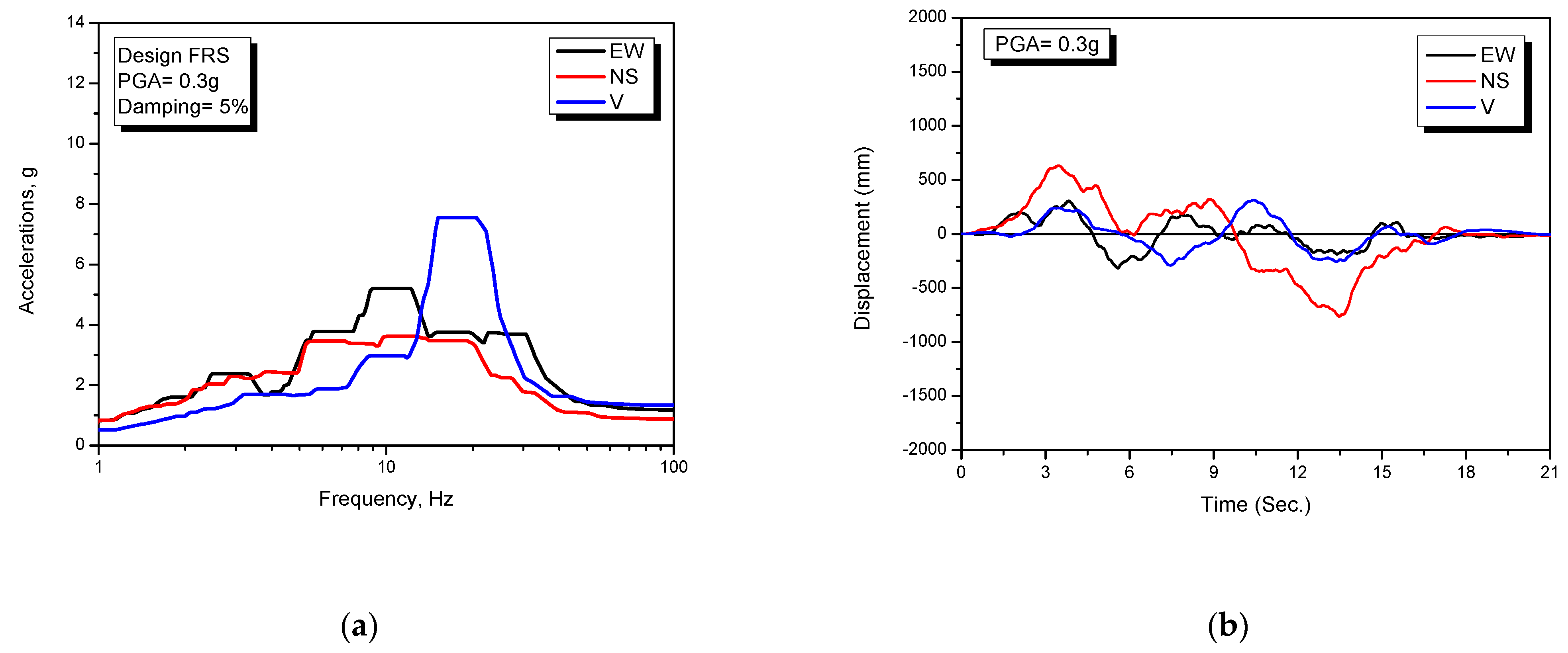
2.2. Load Definition at Component Supports

As one of the main procedures calculating the seismic HCLPF capacity of the target components, the median in-structure floor response time histories at the reference locations or subsystem support locations are required. Such median floor response time histories are obtained from the system seismic time history analysis with the median ground input motions. There are many scientific studies for the ground input motions [19,20,21,22], but the seismic input motions considered in the load definition are based on the required design spectrum by the regulatory bodies such as US NRC RG-1.60 [23].
The median input motions are ultimately used to calculate the median seismic capacity of the components. One of four available cases, as follows, can be used to generate the median in-structure floor response time histories corresponding to the median ground input motions.
  • Case 1: when the site-specific ground response spectrum (GRS) is available.
  • Case 2: when using the uniform response spectrum (URS) in NUREG/CR-0098 [24].
  • Case 3: when only design floor response spectrum is available.
  • Case 4: when floor response time histories are available.

2.2.1. For Case 1

When the site-specific GRS is available, the system seismic analyses shall be performed for at least more than five sets of the ground artificial time histories obtained from the site-specific GRS in order to determine the median floor response time histories at the reference locations or subsystem support locations.
The determined median time histories of in-structure motions may be used as excitations for subsystem seismic analysis. For the seismic time history analyses of subsystems using the median time histories of in-structure motions, an equivalent procedure to peak broadening and enveloping of design floor response spectra or peak shifting of raw response spectra should be used complied with the ASCE 4–16 C6.3.2 [25].

2.2.2. For Case 2

When the ground input motions of the NUREG/CR-0098 URS are used for the system seismic analysis, a single set of three directional ground artificial time histories to match URS as complying with the provisions of RG 1.122 [26] to account for uncertainty can be used for the system seismic analysis to generate the median in-structure seismic input motions at subsystem support locations.
Alternatively, multiple sets of three directional ground artificial time histories derived from URS can be used to determine the median floor responses obtained from the multiple system seismic analyses (each of which used one of the multiple sets of ground time histories).

2.2.3. For Case 3

In the case where only design floor response spectra obtained from the system seismic analysis using the RG 1.60 design spectrum [23] are available, the median floor response spectrum can be determined from the design floor response spectrum by multiplying the adjust factor, fm obtained as follows;
f m = Ratio   of   Spectral   Peak = ( A URS A RG 1.60 ) anchored   at   PGA
This method is applicable only when the in-structure design floor response spectrum is obtained from the elastic system seismic analysis.
The synthetic median floor response time histories can be generated for use in time history analyses of singly supported subsystems or multiply supported subsystems analyzed by using a single excitation whose response spectrum envelops the spectra at all support locations. In general, the generation of synthetic in-structure floor response time histories consists of the following steps:
  • Develop or obtain the floor response spectra for the subsystem support locations at which time histories are required;
  • If a single time histories are to be generated for multiple support locations, develop spectra that envelope all spectra at these locations;
  • Modify the floor response spectra in accordance with ASCE 4–16 Section 6.2.3 [25] to account for uncertainties associated with supporting soil and structures and their analysis; and
  • Generate the synthetic floor response time histories in accordance with the requirements of ASCE 4–16 Chapter 2.

2.2.4. For Case 4

In the case where the floor response time histories at support locations obtained from the system seismic analysis by using the RG1.60 design spectrum [23] are available, the median floor response time histories can be determined by scaling the adjust factor, fm of Equation (3).
This method is applicable only when the floor response time histories are obtained from the elastic system seismic analysis.
The determined median time histories of in-structure motions may be used as excitations for subsystem seismic analysis. For the seismic time history analyses of subsystems using the median time histories of in-structure motions, an equivalent procedure to peak broadening and enveloping of the floor response spectra or peak shifting of raw response spectra should be used, complying with the ASCE 4–16 C6.3.2.

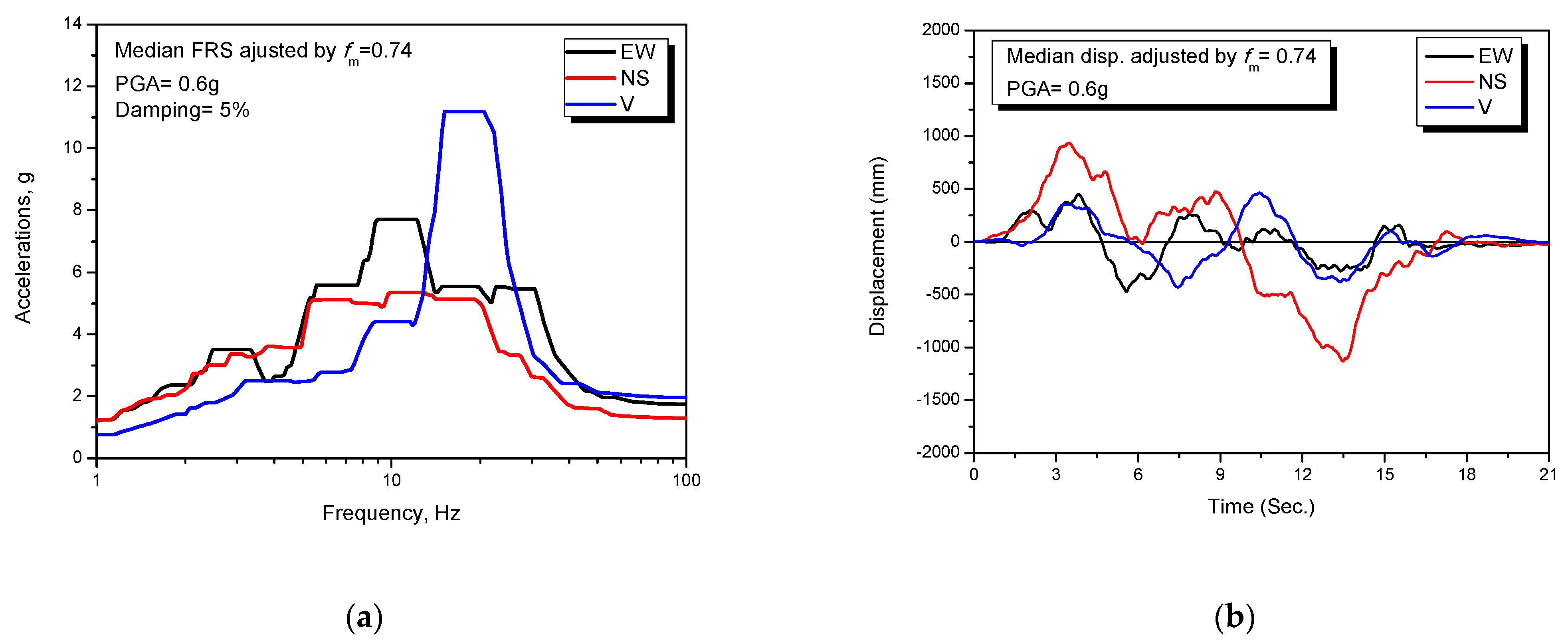
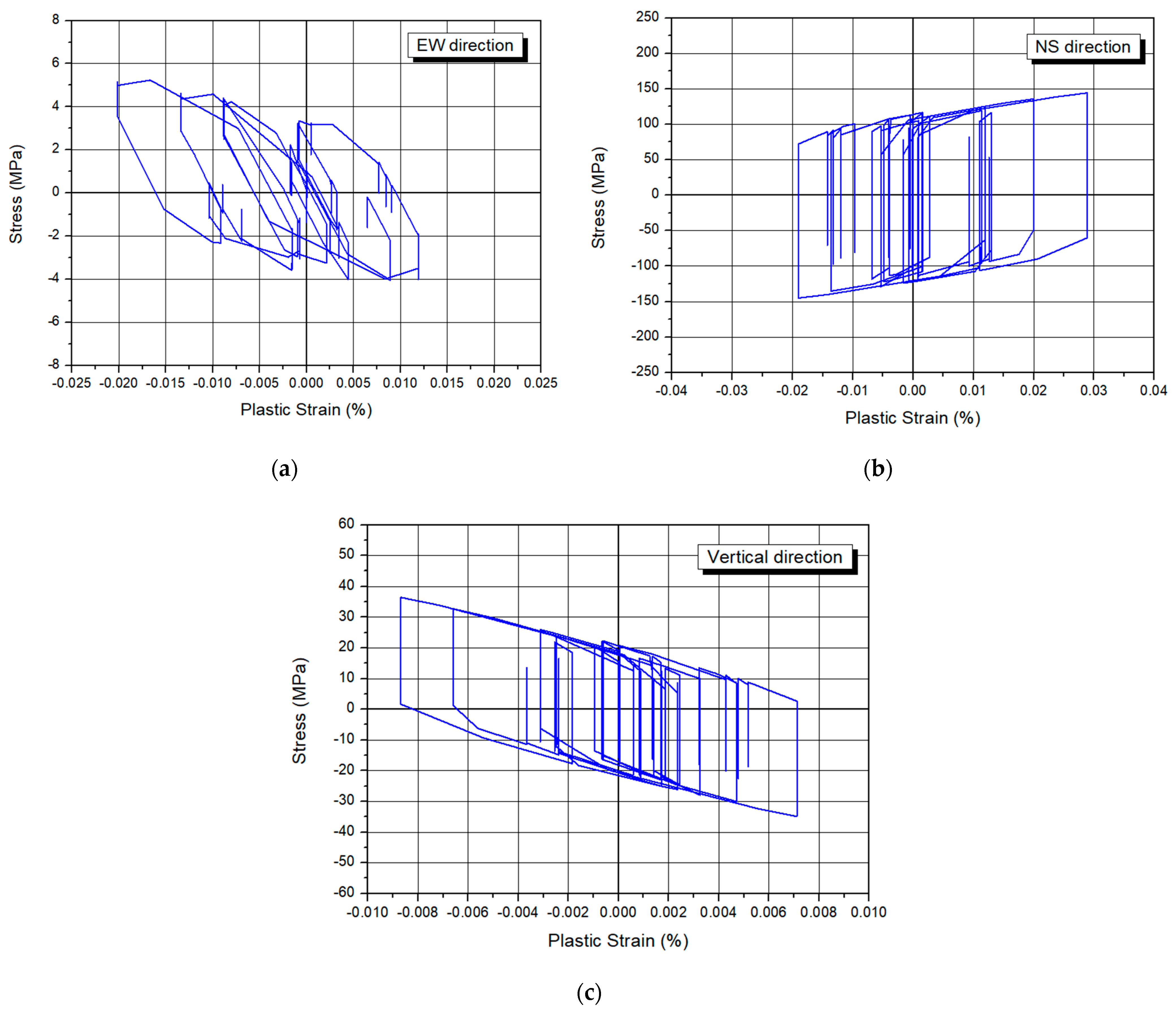
2.3. Median Seismic Demand Calculation

The first task in the seismic FA is to estimate the median seismic demand at the location occurring the maximum accumulated equivalent plastic strain based on the reference earthquake input level described in above Section 2.2. A general procedure for evaluating the median seismic demand is provided in Steps 1 through Step 4 below.
Step 1: Define the floor response time histories as the reference at the component support locations with one of the ways provided in the above Section 2.2. If there are the non-reversing dynamic loads to be combined with the reference earthquake input, the floor response time histories required as input motions should be generated synthetically from the response spectra enveloping the design floor response spectra and the non-reversing dynamic events spectra.
Step 2: Perform the component seismic time history response analysis for the floor response time histories with proper boundary conditions, initial conditions, and the inelastic material models. In the analysis, the median damping value should be used. The damping values specified in NRC RG 1.61 [27] might be applicable for the specific components.
Step 3: Determine the critical location from the point occurring the maximum accumulated equivalent plastic strain value.
Step 4: Calculate the median seismic demands for two failure modes as follows;
For   ductile   fracture   failure   mode : D M 1   =   [ T F ( t )   ε eq p ( t ) ] max
For   fatigue-induced   failure   mode : D M 2   =   [ T F ( t ) ] avg   [ ε eq t ( t ) ] max  
In the above equations, the strain responses are considered due to the seismic loads except normal sustained loads. The detailed method and example calculating DM1 and DM2 values are well described in the previous study [17].

2.4. Allowable Strain Capacity Calculation

A general procedure for calculating the allowable strain capacity for the metal component is described in Steps 1 and 2 below.
Step 1: Determine the total equivalent elastic strain for the sustained loads, which shall be simultaneously considered during the seismic events.
Step 2: As shown in the design acceptance criteria of Equations (1) and (2), determine the allowable strain capacities (CM1 and CM2) for two failure modes as follows;
For   ductile   fracture   failure : C M 1 = ε u + 0.25 ( ε f ε u )
For   fatigue-induced   failure : C M 2 = ε a [ T F ( t ) ] avg [ ε eq e ] sustained
In the case of the fatigue-induced failure mode, the allowable strain capacity for the seismic load should be the value subtracted from the value of an averaged triaxiality factor multiplied with elastic strain due to the sustained loads such as dead weight and internal pressure from the total allowable strain as shown in Equation (7). The detailed procedure and example for calculating CM1 and CM2 values are well described in the previous study [17].

2.5. Median Seismic Capacity

The median seismic capacity of the target component is obtained using the median values for all basic variables in the deterministic analysis. This procedure follows the same steps that an engineer would typically perform in a conventional seismic design or analysis, except that different input motions and allowable capacities are used.
In a seismic FA, the goal is to obtain the median seismic capacity in terms of a defined ground motion variable (e.g., PGA or average spectral acceleration). The engineer starts with a reference earthquake input that is a site-specific response spectrum shape anchored to a reference PGA value. In one approach, the analyst may use the original design results as the basis for the seismic FA. Here, the conservatism is removed at each step, and the reference ground response spectrum is scaled to a median capacity.
The reference earthquake input is scaled until the component just reaches the failure level. The median seismic capacity is just the scaled reference ground response spectrum, where the scale factor is based on a deterministic analysis substituting median values for each of the basic variables. The reference earthquake parameter should be the same one as used in the hazard analysis.
Step 1: The factor of safety (i.e., earthquake scale factor), (FS)ref for the target component shall be determined as follows;
( F S ) ref = Min [ C M 1 D M 1   ,   C M 2   D M 2 ]  
Step 2: The median seismic capacity, (SC)M for the base case is calculated from the results of the factor of safety (FS)ref obtained from above Step 1 as follows;
( S C ) M = F μ   ( F S ) ref   A ref
In equation (9), Fμ and Aref indicate a factor of inelastic energy absorption in the building structures and a referenced ground acceleration, respectively. In some cases, the Aref can be the value anchored to the median averaged spectral acceleration or the median peak ground acceleration used for the base case.
In the above calculation, the inelastic energy absorption factor, Fμ is introduced to account for the factor that an earthquake represents a limited energy source and the in-structure building supporting the target components are capable of absorbing substantial amounts of energy beyond yield without loss-of-function [28,29]. Related to the target metal components, the capacity of the inelastic energy absorption is already considered in the inelastic seismic analysis with the material constitutive models used in this study.

2.6. Variables of Logarithmic Standard Deviation

The procedures used to calculate the logarithmic standard deviations for randomness and uncertainty are based on the recommendation procedures in reference 1 using the approximate second-moment method. The basic variable logarithmic standard deviations are provided in Table 1. For each of the demand random variables, the corresponding parameter is increased by a factor corresponding to one standard deviation or appropriate values and the factor of safety recomputed.
To calculate the HCLPF by the seismic FA, the demand variables for the target component shall be clearly defined. Table 1 provides the list of typical basic variables to be defined with a median demand factor and one standard deviation value (1σ).

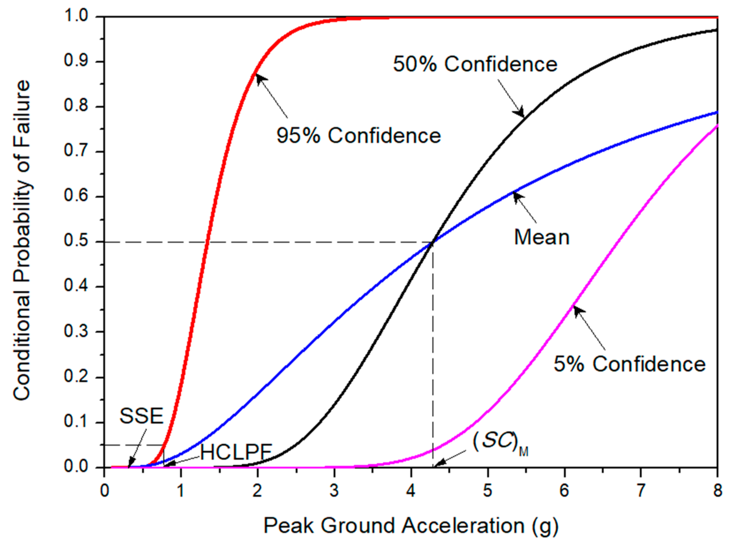
2.7. Calculation of HCLPF

The overall procedures calculating the HCLPF of the target metal component are described as following Step 1 to Step 6.
Step 1: Define the parameter evaluated at 1σ for each variable in Table 1. As an example, when the variables are related with the input seismic loads at the location of the component, the ith parameter corresponding to the logarithmic standard deviation 1σ in Table 1 will be the scaled floor response time histories, [ S I M ¯ ( t ) ] i as follows;
[ S I M ¯ ( t ) ] i = S I M ( t ) e β i
In the above Equation (10), SIM(t) is the median seismic input time histories corresponding to the specific directions, which are used for the calculation of the seismic median capacity as the base case in the above Section 2.6.
Step 2: Perform the inelastic seismic analysis for the scaled input motion [ S I M ¯ ( t ) ] i or other parameters determined at 1σ according to the same procedures of the seismic demand calculation in the above Section 2.3 and calculate the adjusted factor of safety, (FS) by the same procedure of Step 1 in the above Section 2.5.
Step 3: Repeat Step 1 and Step 2 by changing each of the variables one at a time and calculate (FS) value for each variable.
Step 4: Calculate each of the individual βi by using the following equation:
β i = 1 | |   ln [ ( F S ) ref ( F S ) 1 σ ]
The parameter (FS)ref is the factor of safety calculated for the reference earthquake input (i.e., for the median reference case) to reach failure. The (FS) is the adjusted factor of safety calculated for the adjusted earthquake input for the ith variable set at the φ standard deviation (σ) level while all other basic variables are kept at their median levels. The parameter φ is usually set at 1 on the side of the median that leads to the lowest capacity.
Step 5: Calculate the combined logarithmic standard deviation, βR and βU as follows;
β R = ( i β R i 2 ) 1 / 2 , β U = ( i β U i 2 ) 1 / 2
Step 6: Calculate the HCLPF value by the following equation:
H C L P F = ( S C ) M e 1.65 ( β R + β U )

3. Examples of Application

3.1. Description of Example Problem

An example problem investigated in this paper is the safety-related NPP component nozzles connecting the surge line piping to the pressurizer and the hot leg piping system. This component is known to be one of the seismic fragile parts in a nuclear steam supply system.
Figure 2 presents the coupled finite element model including the surge line piping, hot leg surge line nozzle, and pressurizer surge line nozzle. As shown in the figure, there are four support locations for three snubbers (S1NS, S2V, S3EW) and one sway–strut (RNS) in the surge line piping system. They are assumed to be rigid supports during the seismic events and to be the excitation points for the seismic analysis. It is assumed that the seismic inputs are also applied at the end of nozzle models with the same effects through the pressurizer skirt support and the hot leg piping. More details related to the seismic analysis model are described in the previous study [17].
The used inelastic material models are Chaboche’s three-decomposed kinematic hardening model combined with the Voce isotropic hardening model, which is available in the ANSYS program [30]. All parameters required for the constitutive equations are listed in the previous study [17].

3.2. Calculation of Median Seismic Demand as a Reference

Step 1: Median Seismic Loads at Component Supports
In this study, because the only design floor response spectra at component supports were available for the seismic FA, the method of Case 3 in Section 2.2 is used in order to define the median input motions at the component supports, which should be typically obtained from the system seismic analysis with the median seismic ground motion. Figure 3a presents the enveloped design floor response spectra at component supports used in this study, which were obtained from the elastic system seismic analysis with the design floor response spectrum anchored at SSE (0.3 g) in compliance with the US NRC RG 1.60 [23]. Figure 3b presents the artificial displacement seismic time histories corresponding to the design floor response spectrum of Figure 3a.
To obtain the adjust factor (fm) by the ratio of the spectral peak anchored at the PGA between the design response spectrum for seismic design of NPPs provided in NRC-RG 1.60 [23] and the median elastic response spectrum provided in NUREG/CR-0098 [24]. Figure 4 shows the comparison of these two spectra anchored at PGA, 0.3 g. From the figure, the adjust factor is determined to be 0.74 from the ratio of the spectral peak between two spectrum peaks with the assumption that the spectral peak for the design ground motion (RG 1.60) has an averaged value of 0.86 g in the frequency range of 2.5 Hz to 9 Hz specified as control points.
In this paper, in order to enhance the effects of the plastic strain responses in an inelastic seismic analysis approach for the metal components, the reference input motion is taken to be two times of SSE (0.3 g), i.e., anchored at PGA = 0.6 g. Figure 5 presents the used median seismic input motions for the seismic FA as a reference anchored at 0.6 g of PGA, adjusted with the factor of 0.74 from the design floor response spectrum and the artificial displacement seismic time histories of Figure 3.
Step 2: Inelastic Seismic Time History Response Analysis
The inelastic seismic time history response analysis is performed with the median input motion of Figure 5b. In this analysis, the used median damping value for the piping and nozzles is 4% [27]. This is used for the seismic response calculation in the elastic strain region. When the metal components are beyond the elastic strain, the effects of energy dissipations are hysterically applied through the inelastic material models. Figure 6 shows hysteretic response results representing the inelastic material behavior and energy dissipation at the critical location defining at next Step 3 procedure.
Step 3: Determination of the critical location for FA
From the inelastic seismic analysis results, the nodal point representing the maximum accumulative equivalent plastic strain (AEPS) is determined as the critical location. Figure 7 presents the contour plot of the maximum AEPS at the end time of the seismic loads and the critical location for the FA. As shown in the figure, the maximum value occurs at the interface region connecting the safe-end to the nozzle body of the hot leg surge line nozzle.
Step 4: Calculation of the median seismic demands for two failure modes
At the determined critical location, the TF and the AEPS time history responses are calculated as shown in Figure 8.
To determine the maximum total strain (elastic + accumulated plastic) in Equation (5), the maximum equivalent elastic strain should be the sum of the maximum equivalent elastic strain by the inertia seismic load and by the seismic anchor motion at supports. Figure 9 shows the equivalent elastic strain time history responses by the inertia seismic load at the critical location shown in Figure 7b and gives the maximum value of 0.075%. From the quasi-static analysis for the anchor motion for the two times SSE load, the calculated equivalent elastic strain was 0.037% [17] and there was no plastic strain response at the critical location. Considering the adjust factor of 0.74, the median elastic strain due to the seismic anchor motion is estimated to be 0.024%. Then, the maximum total elastic strain is 0.112%.
From the calculated TF and strain values, the median seismic demands for each failure mode are determined as follows;
For ductile fracture failure mode (DM1):
  D M 1   =   [ T F ( t )   ε eq p ( t ) ] max   =   ( 8.25   ×   0.24 ) t = 14.275 s   =   1.98 %
For fatigue-induced failure mode (DM2):
D M 2 = [ T F ( t ) ] avg   [ ε eq t ( t ) ] max   = [ T F ( t ) ] avg   [ ε eq e   +   ε eq p ( t ) ] max = 1.421   ( 0.102   +   0.26 ) = 0.514 %

3.3. Calculation of Allowable Strain Capacity

Step 1: Calculation of total equivalent elastic strain for the normal sustained loads
The normal sustained loads for Service Level A and Level B [31], which are considered in the nuclear component design, are typically the dead weight and the internal pressure. For these loads, plastic deformation is not basically allowed for the design of the nuclear metal components. Therefore, the seismic demand due to the elastic strain by the normal sustained loads should be considered in the determination of the allowable strain capacity for a fatigue-induced failure mode.
In this study, the constant spring hangers, which maintain a balance of an equal pipe weight during the seismic event, are used for the surge line, therefore the effect of the dead weight on the critical location of the nozzle is neglected and is assumed to be zero. The design internal pressure is 15.5 MPa and it results in an elastic strain of 0.033% at the critical location [17].
Step 2: Determined the allowable strain capacities
The allowable strain capacities are determined from the design limit criteria of Equations (1) and (2) for two failure modes as follows;
For ductile fracture failure mode (CM1):
C M 1 =   ε u + 0.25 ( ε f   ε u ) = 30 + 0.25 ( 40 40 ) = 32.5 %
For fatigue-induced failure (CM2):
C M 2 = ε a [ T F ( t ) ] a v g [ ε e q e ] s u s t a i n e d = [ S a ( 20 ) ] a E K y [ T F ( t ) ] a v g [ ε e q e ] s u s t a i n e d   = [ 4300 e 6 ]   1.5 195 e 9   ( 0.9 ) 1.421   x   0.033   = 2.980 0.047         = 2.933 %  
For a calculation of the CM2, the allowable stress range, Sa, is determined to be corresponding to the number of cycles of 20 from the design fatigue curve of the ASME Section III Appendices, Mandatory Appendix I, Figure I-9.1 [32]. The factor of a is chosen to be 1.5 for a material of low alloy steel used in this study. The factor of Ky, which is the value in order to compensate for the effects of the elastic modulus between the design fatigue curve and the used value in actual seismic analysis, is 0.9.

3.4. Determination of the Median Seismic Capacity as Reference Case

Step 1: Calculation of the factor of safety: (FS)ref
From the calculation results of the seismic demands and the allowable strain capacities at the critical location, the factor of safety using as an earthquake scale factor is determined as follows;
( F S ) r e f = M i n [ C M 1 D M 1   ,   C M 2   D M 2 ] = M i n [ 32.5 1.98   ,   2.933   0.514 ] = 5.703
Step 2: Calculation of the median seismic capacity: (SC)M
Based on the calculated factor of safety in Step 1, the median seismic capacity, which will be the reference case for the HCLPF calculation through the seismic FA, is determined as follows;
( S C ) M = F μ   ( F S ) ref   A ref = 1.25 × 5.703   ×   0.6   g   = 4.277   g
In the above calculation, the inelastic energy absorption factor, Fμ is conservatively considered to be 1.25 as long as the structure building supporting the target components is ductile as recommended in EPRI NP-6041 [33].

3.5. Definition of the Variables of Logarithmic Standard Deviation

To carry out the seismic FA by the commonly used probabilistic approach, individual variables are defined with some appropriate assumptions, affecting the target component’s seismic responses.
Table 1 presents the variables and the defined logarithmic standard deviations for randomness (βR) and uncertainty (βU) corresponding to 1σ in this study.
The variables for the ground motion and the structural response in Table 1 are derived from parameters determined for the design floor response spectrum at locations of the target components. The variables for the component response are derived from the parameters determined from the seismic strain responses at the location of a critical metal component.

3.5.1. Variables for Ground Motion

For the ground motion, the variable of the earthquake response spectrum shape (FERSS) is generically considered to take into account the fact that a real earthquake, in general, will be different from the smooth reference ground input motion used in the FA. In order to account for this variability, the values of the logarithmic standard deviation are specified to be 0.2 both for the peak valley randomness, βR, and the spectral shape uncertainty, βU, which are based on the typical ranges depending on the horizontal frequencies given in the EPRI/TR-103959 [15]. The dominant horizontal natural frequencies in this example are 20.3 Hz for EW direction and 48.0 Hz for NS direction. Therefore, the used value of 0.2 will be conservatively the upper bound value fully covered the typical ranges (0.12~0.19) given in the EPRI/TR-103959.
Since the horizontal ground response spectrum is assumed to be the average of the two horizontal directions, the smooth referenced response spectrum for one direction can be higher than the other perpendicular direction in a real earthquake. This can result in a randomness variability in seismic response. Therefore, the horizontal direction peak response (FHDPR) due to the different orthogonal two horizontal spectrum shapes is considered to be the basic variable in this example. Corresponding randomness, βR, value is recommended between 0.12 and 0.14 in the EPRI/TR-103959. Through the detailed modal analysis for an example in this study, it was found that the seismic responses at the critical location in the hot leg nozzle are dominantly affected by the vertical mode of 7.7 Hz of the surge line piping. Therefore, the value of the randomness, βR, for this variable is selected to be 0.12 as a lower bound in the EPRI/TR-103959.
When the vertical earthquake component is assumed to be equal to 2/3 times the horizontal component at the ground level, the ranges of the βR and βU are recommended to be 0.22~0.28 and 0.20~0.26, respectively [15]. However, recent seismic design in the NPPs requires the V(Vertical)/H(Horizontal) ratio to be 1.0 and the same frequency contents of the horizontal component. Therefore, the randomness and the uncertainty in the vertical ground response spectrum shape are already considered in the variables of FERSS and FHDPR and then the variable of the vertical component responses (FVCR) is assumed to be 0.1 for all randomness eliminating a separate uncertainty term for simplicity.

3.5.2. Variables for Structural Building Response

For the structural building response, the median damping value for the reinforced concrete, in general, is 5% and a corresponding logarithmic standard deviation based on −1σ is assumed to be 3.5%. From the system modal analysis, the horizontal frequencies of the in-structure building installing the target component were 9.7 Hz for EW direction and 6.3 Hz for NS direction. Then, from the spectrum amplification factors (Sa) for the horizontal elastic response of the median (50%) acceleration values given in the NUREG/CR-0098 [24], the values of the uncertainty, βU for the damping variable (FSD) are determined to be 0.11 as follows;
For   horizontal   EW   direction : β U = 1 | Φ | ln   [ S a ( 9.7   Hz ,   3.5 % ) S a ( 9.7   Hz ,     5 % ) ] = 1 1 ln [ 2.36 2.12 ] = 0.11 For   horizontal   NS   direction : β U = 1 | Φ | ln   [ S a ( 6.3   Hz ,   3.5 % ) S a ( 6.3   Hz ,     5 % ) ] = 1 1 ln [ 2.36 2.12 ] = 0.11
In the above, the symbol of Φ indicates the number of standard deviations.
The variable of the modeling in the seismic response is primarily related to the uncertainty in the mode shapes and the modal frequencies of the actual structural building. In general, it can be assumed that the finite element modeling of the nuclear reactor building, which is required to be modeled with a fully three-dimensional seismic analysis model accounting for the detailed stiffness and mass distributions of the actual structural building, is median-centered in the region of the elastic behavior without any conservative bias [15]. Therefore, for the variable of the modeling in the structural building response (FSM), the uncertainty, βU, is assumed to be 0.07 in this study.
In actuality, the uncertainty in the modal frequencies affects the structural seismic responses and depends on the mass and stiffness modeling. This is already considered in the variable of the modeling, FSM, and is not included in this study.

3.5.3. Variables for Component Response

Fundamentally, in this paper, the seismic FA method used for the nuclear metal components is based on the seismic strain calculations by the inelastic seismic time history analysis applying three independent directional input motions simultaneously at the supports of the target component. Therefore, the consideration of the uncertainties for the modal combination is not necessary. In this study, the same variables for the structural building response are considered for the component, as shown in Table 1.
For the variable of damping in component response, it is assumed that the standard deviation for −1σ is equivalent to the effect of 10% lowering the first modal frequency of the target component in the Rayleigh damping model. The uncertainty of the modal frequency can significantly affect the Rayleigh damping parameters and eventually influence in the calculation of the inelastic seismic strain responses [17].

3.6. Calculation of HCLPF

From the determined variables in Table 1, the HCLPF is calculated according to the procedures of Step 1 through Step 6 described in Section 2.7. To do this, the factors of safety (FS) for the variability corresponding to one standard deviation (1σ) are calculated at first for individual βi in Table 1.
As an example calculation for the variable of FERSS in Table 1, the component inelastic seismic time history analysis is carried out for the input loads, (ATH)EW and (ATH)NS which are the scaled input displacement time histories of Figure 5b by the variability of one standard deviation(1σ) only for two horizontal directions. As the randomness and the uncertainty have the same variability for this variable, with the results of the seismic strain responses at the critical location, the factor of safety, (FS) both for the randomness(βR) and the uncertainty (βU) are calculated to be 3.980 by the same procedures in Section 3.2 through Section 3.4: (DM2) = 0.754%, (CM2) = 2.932%. Then, the logarithmic standard deviation values for this variable are estimated as follows;
β R = β U = 1 | |   l n [ ( F S ) r e f ( F S ) 1 σ ] = 1 1   l n [ 5.703 3.890 ] = 0.382
For all the other variables, the logarithmic standard deviation values for the randomness and uncertainty variability can be estimated by the same method used for the FERSS.
Table 2 reveals the calculation summaries required to calculate the logarithmic standard deviations for each variable. Table 3 presents the calculation results of the logarithmic standard deviation values for each variable.
From the results of Table 3, the combined logarithmic standard deviation, βR and βU are calculated as follows;
β R = ( i β R i 2 ) 1 / 2 = ( 0.382 2 + 0.232 2 + 0.235 2 ) 1 / 2 = 0.330 β U = ( i β U i 2 ) 1 / 2 = ( 0.382 2 + 0.419 2 + 0.286 2 + 124 2 + 0.286 2 ) 1 / 2 = 0.707
With the results of the median seismic capacity, (SC)M and the value of the logarithmic standard deviation(LSD), βR and βU, representing the variability, the HCLPF value is calculated as follows;
H C L P F = ( S C ) M e 1.65 ( β R + β U ) = 4.277   e 1.65 ( 0.330 + 0.707 ) = 0.772   g
As shown in the result, the HCLPF capacity of the target component studied in this paper is 0.772 g, which is the earthquake level anchored at PGA corresponding approximately to a 95 percent confidence that the probability of failure is less than 5 percent. Table 4 presents the summary results of the exampled FA in this study.
Graphically understanding the results of the exampled FA of Table 4, the fragility curves representing the conditional probability of failure (Pf) are presented in Figure 10, obtained from the equation as follows [34];
P f = Φ [ ln [ A / ( S C ) M ] + β U Φ 1 ( Q ) ] β R ]
where A, Φ[], Φ−1 and Q represent PGA value, the standardized normal distribution function, the inverse normal (Gaussian) distribution function, and the specific confidence level, respectively.
The mean fragility curve in Figure 10 is obtained from the equation as follows;
P f = Φ [ ln [ A / ( S C ) M ] β C ]
where
β C = ( β R 2 + β U 2 ) 1 / 2 = 0.78
The results of the fragility curves in Figure 10 can be used for the reliability analysis of the nuclear components [35].

4. Conclusions

In this study, the detailed probabilistic seismic FA procedures applicable for the pressure retaining nuclear metal components, which can evaluate the seismic HCLPF capacity value, are established with the strain-based failure modes such as ductile fracture failure and fatigue-induced failure.
Through step-by-step calculations for the exampled surge line nozzles, it is found that the inelastic strain-based seismic FA approach gives somewhat large variability of the logarithmic standard deviations in randomness and uncertainty due to the sensitive inelastic strain response at the plastic region, but the strain-based limit criteria adequately assure the HCLPF seismic capacity. In actuality, the design-basis earthquake is 0.3 g (SSE) in this example component, but the actual calculated seismic capacity corresponding approximately to a 95 percent-confidence probability of failure of less than 5 percent is 0.772 g, which is more than twice the design level. Therefore, it is expected that the seismic FA approach investigated in this paper can be used as one of the candidate alternative rules for the highly increased design-basis earthquake or beyond-design-basis earthquake.
Through this study, further studies are recommended for more practical application of these proposed procedures to the nuclear facility components as follows;
  • Determination of median input motions for component seismic fragility analysis
  • Material parameter identifications for inelastic material model
  • Sensitivity studies on inelastic seismic responses with finite element models
  • Detailed investigations for the variable definitions of ground motions, building structures, and components,
  • Determination of logarithmic standard deviation value corresponding to the variables.

Author Contributions

Conceptualization, G.-H.K., S.K., and H.-S.N.; methodology, G.-H.K. and S.K.; validation, G.-H.K.; formal analysis, G.-H.K.; investigation, S.K. and H.-S.N.; writing—original draft preparation, G.-H.K.; writing—review and editing, S.K. and H.-S.N.; funding acquisition, G.-H.K. All authors have read and agreed to the published version of the manuscript.

Funding

This study was funded by the Ministry of Trade, Industry and Energy through KETEP (Korea Institute of Energy Technology Evaluation Planning) (No. 20181510102380).

Institutional Review Board Statement

Not applicable.

Informed Consent Statement

Not applicable.

Acknowledgments

This study was supported by the Ministry of Trade, Industry and Energy through KETEP (Korea Institute of Energy Technology Evaluation Planning) (No. 20181510102380).

Conflicts of Interest

The authors declare no conflict of interest.

References

  1. ASME BPVC Section III Appendices. Nonmandatory Appendix EE: Strain-Based Acceptance Criteria Definitions and Background Information; ASME: New York, NY, USA, 2019. [Google Scholar]
  2. ASME BPVC Section III Appendices. Nonmandatory Appendix FF: Strain-Based Acceptance Criteria for Energy-Limited Events; ASME: New York, NY, USA, 2019. [Google Scholar]
  3. ASME B&PV Code Committee. Alternative Rules for Level D Service Limits of Class 1, 2, and 3 Piping Systems; Section III, Division 1, ASME Code Case(Record No. 13–1438); ASME: New York, NY, USA, 2019. [Google Scholar]
  4. Masaki, M.; Akihiro, O.; Tomoyoshi, W.; Izumi, N.; Tadahiro, S.; Masaki, S. Seismic Qualification of Piping Systems by Detailed Inelastic Response Analysis: Part 1–A Code Case for Piping Seismic Evaluation Based on Detailed Inelastic Response Analyses. In Proceedings of the ASME 2017 PVP Conference, Waikoloa, HI, USA, 16–20 July 2017. [Google Scholar]
  5. Srinivasan, R.; Selman, P.B. Design Basis vs. Beyond Design Basis Considerations for Operating Plants. Transactions. In Proceedings of the SMiRT-23 Conference, Manchester, UK, 10–14 August 2015. [Google Scholar]
  6. ASME BPVC Section III Appendices. Mandatory Appendix XXVII: Design by Analysis for Service Level D; ASME: New York, NY, USA, 2019. [Google Scholar]
  7. Zhao, C.; Yu, N.; Oz, Y.; Wang, J.; Mo, Y.L. Seismic fragility analysis of nuclear power plant structure under far-field ground motions. Eng. Struct. 2020, 219, 110890. [Google Scholar] [CrossRef]
  8. Kim, S.W.; Jeon, B.G.; Hahm, D.G.; Kim, M.K. Seismic fragility evaluation of the base-isolated nuclear power plant piping system using the failure criterion based on stress-strain. Nucl. Eng. Technol. 2019, 51, 561–572. [Google Scholar] [CrossRef]
  9. Wang, Z.; Pedroni, N.; Zentner, I.; Zio, E. Seismic fragility analysis with artificial neural networks: Application to nuclear power plant equipment. Eng. Struct. 2018, 162, 213–225. [Google Scholar] [CrossRef] [Green Version]
  10. Park, J.; Towashiraporn, P.; Craig, J.I.; Goodno, B.J. Seismic fragility analysis of low-rise unreinforced masonry structures. Eng. Struct. 2009, 31, 125–137. [Google Scholar] [CrossRef]
  11. Tolentino, D.; Marquez-Dominguez, S.; Gaxiola-Camacho, J.R. Fragility Assessment of Bridges Considering Cumulative Damage Caused by Seismic Loading. Eng. Struct. 2020, 24, 551–560. [Google Scholar] [CrossRef]
  12. Xu, J. Guidance on Probabilistic-Risk-Assessment-Based Seismic Margin Assessments for New Reactors. Transactions. In Proceedings of the SMiRT-21 Conference, New Delhi, India, 6–9 November 2011. [Google Scholar]
  13. Electric Power Research Institute. Seismic Probabilistic Risk Assessment Implementation Guideline; Report 3002000709; Electric Power Research Institute (EPRI): Palo Alto, CA, USA, 2013. [Google Scholar]
  14. American Society of Civil Engineers. Seismic Analysis of Safety-Related Nuclear Structures; ASCE/SEI Standard 4–16; ASCE: Reston, VA, USA, 2017. [Google Scholar]
  15. Electric Power Research Institute. Methodology for Developing Seismic Fragility; EPRI/TR-103959; Electric Power Research Institute (EPRI): Palo Alto, CA, USA, 1994. [Google Scholar]
  16. ASME. Companion Guide to ASME Boiler Pressure Vessel Code; ASME: New York, NY, USA, 2009. [Google Scholar]
  17. Koo, G.H.; Kim, J.S.; Kim, Y.J. Feasibility Study on Strain-Based Seismic Design Criteria for Nuclear Components. Energies 2020, 13, 4435. [Google Scholar] [CrossRef]
  18. Electric Power Research Institute. Seismic Fragility Application Guide; EPRI/TR-1002988; Electric Power Research Institute (EPRI): Palo Alto, CA, USA, 2002. [Google Scholar]
  19. Barone, G.; Iacono, F.L.; Navarra, G.; Palmeri, A. Closed-form stochastic response of linear building structures to spectrum-consistent seismic excitations. Soil Dyn. Earthq. Eng. 2019, 125, 105724. [Google Scholar] [CrossRef]
  20. Barone, G.; Iacono, F.L.; Navarra, G.; Palmeri, A. A novel analytical model of power spectral density function coherent with earthquake response spectra. In Proceedings of the 1st International Conference on Uncertainty Quantification in Computational Sciences and Engineering (UNCECOMP), Crete Island, Greece, 25–27 May 2015. [Google Scholar]
  21. Muscolino, G.; Genovese, F.; Biondi, G.; Cascone, E. Generation of fully non-stationary random processes consistent with target seismic accelerograms. Soil Dyn. Earthq. Eng. 2021, 141, 106467. [Google Scholar] [CrossRef]
  22. Zhang, R.; Zhang, L.; Pan, C.; Chen, Q.; Wang, Y. Generating high spectral consistent endurance time excitations by a modified time-domain spectral matching method. Soil Dyn. Earthq. Eng. 2021, 145, 106708. [Google Scholar] [CrossRef]
  23. Nuclear Regulatory Commission. Design Response Spectra for Seismic Design of Nuclear Power Plants; Regulatory Guide 1.60; Nuclear Regulatory Commission: Rockville, MD, USA, 1973.
  24. Nuclear Regulatory Commission. Development of Criteria for Seismic Review of Selected Nuclear Power Plants; NUREG/CR-0098; Nuclear Regulatory Commission: Rockville, MD, USA, 1978.
  25. ASCE. Seismic Analysis of Safety-Related Nuclear Structures, ASCE Standard; ASCE/SEI 4–16; ASCE: Reston, VA, USA, 2017. [Google Scholar]
  26. Nuclear Regulatory Commission. Development of Floor Design Response Spectra for Seismic Design of Floor-Supported Equipment or Components; Regulatory Guide 1.122; Nuclear Regulatory Commission: Rockville, MD, USA, 1978.
  27. Nuclear Regulatory Commission. Damping Values for Seismic Design of Nuclear Power Plants; Regulatory Guide 1.61; Nuclear Regulatory Commission: Rockville, MD, USA, 2007.
  28. Newmark, N.M. Inelastic Design of Nuclear Reactor Structures and Its Implications on Design of Critical Equipment. Transactions. In Proceedings of the SMiRT-4 Conference, San Francisco, CA, USA, 15–19 August 1977. [Google Scholar]
  29. Riddell, R.; Newmark, N.M. Statistical Analysis of the Response of Nonlinear Systems Subjected to Earthquakes; SRS-468; Department of Civil Engineering, University of Illinois: Champaign, IL, USA, 1979. [Google Scholar]
  30. ANSYS. ANSYS Mechanical APDL Release 15.0; ANSYS, Inc.: Canonsburg, PA, USA, 2014. [Google Scholar]
  31. ASME BPVC Section III, Division 1. Subsection NB: Class 1 Components; ASME: New York, NY, USA, 2019. [Google Scholar]
  32. ASME BPVC Section III Appendices. Mandatory Appendix I: Design Fatigue Curve; ASME: New York, NY, USA, 2019. [Google Scholar]
  33. Electric Power Research Institute. A Methodology for Assessment of Nuclear Power Plant Seismic Margin (Revision 1); EPRI/NP-6041-SL; Electric Power Research Institute (EPRI): Palo Alto, CA, USA, 1991. [Google Scholar]
  34. Kennedy, R.P.; Ravindra, M.K. Seismic Fragilities for Nuclear Power Plant Risk Studies. Nucl. Eng. Des. 1984, 79, 47–68. [Google Scholar] [CrossRef]
  35. Argyroudis, S.A.; Fotopoulou, S.; Karafagka, S.; Pitilakis, K.; Selva, J.; Salzano, E.; Basco, A.; Crowley, H.; et al. A risk-based multi-level stress test methodology: application to six critical non-nuclear infrastructures in Europe. Nat. Hazards 2020, 100, 595–633. [Google Scholar] [CrossRef]
Figure 1. General procedures of seismic fragility analysis for NSSS metal component.
Energies 14 03269 g001
Figure 2. Seismic finite analysis model and piping support locations.
Energies 14 03269 g002
Figure 3. Used seismic input motions at component supports (PGA = 0.3 g): (a) enveloped design floor response spectrum; (b) corresponding artificial displacement time histories.
Energies 14 03269 g003
Figure 4. Comparison of spectrum shapes between NRC-RG 1.60 and NRC-NUREG-CR-0098.
Energies 14 03269 g004
Figure 5. Assumed reference median seismic input motions at component supports (PGA = 0.6 g): (a) enveloped design floor response spectrum; (b) corresponding artificial displacement time histories.
Energies 14 03269 g005
Figure 6. Hysterical stress-plastic strain response at critical location: (a) EW; (b) NS; (c) vertical.
Energies 14 03269 g006
Figure 7. Contour plots of an accumulated equivalent plastic strain at end of time: (a) at hot leg surge line nozzle; (b) sectional contour (A-A) and critical location for FA.
Energies 14 03269 g007
Figure 8. Seismic time history responses at a critical location: (a) TF; (b) Accumulative equivalent plastic strain.
Energies 14 03269 g008
Figure 9. Von-Mises elastic strain time history response for a reference.
Energies 14 03269 g009
Figure 10. Results of fragility curves presenting SSE (0.3 g) and HCLPF (0.772 g).
Energies 14 03269 g010
Table 1. Variables and corresponding logarithmic standard deviations.
VariablesLogarithmic Standard Deviation
βRβU
For Ground Motion:
Earthquake Response Spectrum Shape (FERSS)0.200.20
Horizontal Direction Peak Response (FHDPR)0.12-
Vertical Component Response (FVCR)0.10-
For Structural Building Response:
Damping (FSD)-0.11
Modeling (FSM)-0.07
Frequency (FSF)--
For Component Response:
Damping (FCD)-D0.9f1: −1σ
Modeling (FCM)-0.07
Modal Combination (FCMC)--
Table 2. Calculation summaries required for factor of safety and logarithmic standard deviation values.
Variables [ ε e q t ( t ) ] max [ ε e q e ] s u s t a i n e d [ ε e q p ( t ) ] max [TF(t)]avgDM2CM2
For reference0.1020.0330.2601.4210.5142.933
FERSS0.1070.0330.4191.4330.7542.932
FHDPR0.1040.0330.3371.4270.6302.933
FVCR0.1050.0330.3651.3840.6512.934
FSD0.1080.0330.4831.3250.7832.936
FSM0.1060.0330.3931.3750.6852.934
FCD0.1040.0330.3001.4400.5822.932
FCM0.1060.0330.3931.3750.6852.934
Table 3. Calculated logarithmic standard deviation values for variables.
VariablesVariable Evaluated at 1σAdjusted Factor of Safety (FS)Logarithmic Standard Deviation
βRβU
For Reference Case 5.703
For Ground Motion:
Earthquake Response Spectrum Shape (FERSS)(ATH)EW e0.2
(ATH)NS e0.2
3.8900.3820.382
Horizontal Direction Peak Response (FHDPR)(ATH)EW e0.12
(ATH)NS e0.12
4.4230.232-
Vertical Component Response (FVCR)(ATH)V e0.14.5090.235-
For Structural Building Response:
Damping (FSD)(ATH)EW e0.11
(ATH)NS e0.11
(ATH)V e0.11
3.751-0.419
Modeling (FSM)(ATH)EW e0.07
(ATH)NS e0.07
(ATH)V e0.07
4.283-0.286
Frequency (FSF)----
For Component Response:
Damping (FCD)D0.9f1:−1σ5.040-0.124
Modeling (FCM)(ATH)EW e0.07
(ATH)NS e0.07
(ATH)V e0.07
4.283-0.286
Modal Combination (FCMC)----
Table 4. Summary of the FA results.
Check ListsResults
PGA for a reference0.6 g
Factor of Safety, (FS)ref5.703
Median Capacity, (SC)M4.277 g
LSD for randomness, βR0.330
LSD for uncertainty, βU0.707
HCLPF = (SC)M e−1.65(βR + βU)0.772 g
Publisher’s Note: MDPI stays neutral with regard to jurisdictional claims in published maps and institutional affiliations.

