Article

Advancing Wind Resource Assessment in Complex Terrain with Scanning Lidar Measurements

1
Fraunhofer Institute for Wind Energy Systems IWES, 27572 Bremerhaven, Germany
2
GEO-NET Umweltconsulting GmbH, 30161 Hanover, Germany
*
Author to whom correspondence should be addressed.
Energies 2021, 14(11), 3280; https://doi.org/10.3390/en14113280
Submission received: 15 February 2021 / Revised: 25 May 2021 / Accepted: 28 May 2021 / Published: 3 June 2021
(This article belongs to the Special Issue Recent Advances in Wind Power Meteorology)

Abstract

:
The planning and realization of wind energy projects requires an as accurate and precise wind resource estimation as possible. Standard procedures combine shorter on-site measurements with the application of numerical models. The uncertainties of the numerical data generated from these models are, particularly in complex onshore terrain, not just rather high but typically not well quantified. In this article we propose a methodology for using a single scanning Doppler wind lidar device to calibrate the output data of a numerical flow model and with this not just quantify but potentially also reduce the uncertainties of the final wind resource estimate. The scanning lidar is configured to perform Plan Position Indicator (PPI) scans and the numerical flow data are projected onto this geometry. Deviations of the derived from the recorded line-of-sight wind speeds are used to identify deficiencies of the model and as starting point for an improvement and tuning. The developed methodology is demonstrated based on a study for a site in moderately complex terrain in central Germany and using two rather different types of numerical flow models. The findings suggest that the use of the methodology and the introduced scanning wind lidar technology offers a promising opportunity to control the uncertainty of the applied flow models, which can otherwise only be estimated very roughly.

1. Introduction

An as accurate and precise as possible estimation of the wind resource, and the calculation of the prospective energy yield based on it, are important prerequisites for the successful design of a wind farm. The difficulty of the task increases with the complexity of the site under consideration, but also with the advancing point in time within the project life cycle at which the estimation takes place. While an initial rough estimate is sufficient at an early stage of the project development, the final realization and financing of the project requires maximum accuracy and, in particular, the lowest possible uncertainty of the forecast values of the expected energy yield. For the German onshore wind market, as an example, this demand increased even more when in 2017—with the EEG-2017 [1]—an auction model was introduced for the remuneration of electricity generated from wind power. Following this, bidders must submit their bid based on their expected energy yield at the time when the auction takes place. As a parallel development, the complexity of the sites that are planned and awarded within the auctions is increasing, as simple sites in flat terrain with comparatively high average wind speeds are already occupied and thus less available. This leaves onshore sites that are characterized by hilly or forested terrain, for example, both of which pose a significant challenge to the estimation of the site-specific wind resource. A typical German onshore site in moderately complex terrain, as it has been studied in more depth also for this article, even combines these two challenges.
Lee and Fields [2] have taken a more global look at the development of wind resource assessment procedures and results and have identified a long-term trend of reduction in an overprediction bias (of the estimated wind resource) whereas the uncertainty associated with the prediction error is prominent. Related improvements during the last decades are found both in modelling and measurement techniques. Depending on the complexity of the terrain, uncertainties in the wind potential estimate can be in the order of 10% which in turn can lead to a 30% uncertainty in the annual energy production considering that the power is proportional to the cube of the inflow wind speed [3]. An uncertainty of this magnitude poses an essential challenge to the financing of a wind project, especially since it occurs at a time when it is not yet clear whether the project will be realized at all.
The wind resource assessment (WRA) as part of a wind project development, regardless of whether a wind farm is planned onshore or offshore, is done according to a standard procedure described in various guidelines. WRA generally refers to the process by which wind power developers estimate the future energy production of a wind farm [4]. A more specific term is pre-construction energy yield assessment (EYA) that not just specifies the purpose but also the time of the assessment. Accordingly, there is also a post-construction EYA which, however, is not dealt with in this article. The same applies to the last part of the WRA, the energy yield calculation. What remains is the consideration of wind conditions, which can be divided into the compilation of a wind database and the numerical modelling of wind conditions. Worth mentioning here are the guideline by MEASNET on the “Evaluation of site-specific wind conditions” first introduced in 2009 and updated in 2016 [5] and the Technical Guideline (TG) 6 on “Determination of Wind Potential and Energy Yield” published by the German body FGW and now available in its 11th revision from 2020 [6]. An international standard is also being developed and is currently available as draft referred to as IEC CD 61400-15 [7].
The various guidelines all agree on the point that the wind resource is estimated based on a combination of measured on-site data and numerical data from suitable models. The numerical data are used on the one hand to extrapolate the measured data spatially, i.e., to transfer them from one site to another (which only provides meaningful results within a certain, terrain-dependent, radius of a few kilometers maximum). On the other hand, a temporal extrapolation or so-called long-term correction is carried out on this basis of combined on-site and long-term data, which is necessary because measurements are usually only available for a period in the order of one year, but the wind potential must be estimated for about 20 years. For both aspects, the measurement data are used to calibrate the numerical data and thus reduce the uncertainty of the wind potential estimation. The overall uncertainty can be reduced accordingly by improving the measurement, which can be realized by selecting the most accurate measurement technology or by performing measurements that cover the future wind turbine (WT) sites as accurately as possible. With the latter it is not just referred to the measurement height, which should be at least the hub height of the turbines—getting higher and higher, especially in complex terrain—and in the best case the entire vertical extent of the rotor, but also the horizontal positions in the terrain. It was e.g., shown in [8] that especially in complex terrain it is usually no longer sufficient to measure at just one position, as it is realized with a meteorological (met) mast equipped with anemometers along a vertical line or with a single vertically profiling lidar or sodar device. Similarly, it was explored in [9] how adding an additional measurement to a met mast in complex terrain positively affects the wind resource assessment. In general, and confirmed by the mentioned studies, a conceivable solution to improve the wind potential estimation is the use of different measuring positions, either with simultaneous measurements using several measuring systems, or the repositioning of one measuring system, which is possible at least with remote sensing devices and wind lidars or sodars in particular. TG 6 takes this option into account as a so-called additional measurement (opposed to the main measurement), which can be carried out for the purpose of vertical extrapolation and/or time series extension, whereby the latter also includes horizontal extrapolation. In the case of a planned wind farm consisting of several wind turbines, the main measurement could be carried out at the position of one turbine, while the additional measurements cover the other turbines.
As also pointed out by Lee and Fields [2] and the references given herein, the industry has recognized the role of remote sensing instruments in reducing the uncertainty of energy production and wind speed from extrapolation, such as profiling lidars, scanning lidars, and airborne drones. While (vertically) profiling lidars—just like sodars, which are still of great importance in at least some parts of the industry [10]—can be seen as practical and most cost-efficient replacement of tall met masts, scanning lidars come along with totally new opportunities. In this article, we show how a single additional scanning lidar device can be used to calibrate the output data of a numerical flow model and with this potentially reduce the uncertainties of the final wind resource estimate. The exact methodology for this, as well as the measurement principle of a scanning lidar and how we have applied it here, will be explained in the next section.
An alternative approach, as e.g., pursued in [11], is to use a set of several scanning lidar devices in a synchronized way to produce several so-called virtual met masts at the different locations of interest at a site. Typically, two scanning lidar devices are used together in the dual-Doppler approach. While both alternative approaches pursue the goal of better resolving the wind flow over the terrain with measurements, we consider the first approach and the one followed in the study reported here to be more cost-efficient, since the use of scanning lidar technology in particular drives up the costs of a WRA measurement campaign. Since the measurement costs are at the same time the main part of the budget for a WRA study, additional costs must be regarded as a significant risk for the developer. On the other hand, the use of the technology offers a very good opportunity to quantify the uncertainty of the applied flow models, which can otherwise only be estimated very roughly. This aspect will be taken up again and elaborated on in the discussion at the end of this article.
The article is organized as follows: In Section 2, following this introduction, we introduce the materials (basically measurements and data) and methods relevant to this study. Results are presented in Section 3 and discussed in Section 4, Section 5 rounds off the article with the main conclusions.

2. Materials and Methods

Before we go into more detail about the data studied for this article in Section 2.2, we describe the methodology developed and applied in Section 2.1.

2.1. Methodology

As pointed out in Section 1, the methodology we have developed is about using a single scanning lidar device, in addition to a reference measurement, to calibrate the output data of a numerical flow model. The details of the scanning lidar measurements, together with the specifications of the reference measurement, are further described in Section 2.1.1. In Section 2.1.2, we go into more detail about the use of the numerical model data, and in Section 2.1.3 about the calibration process considered here.

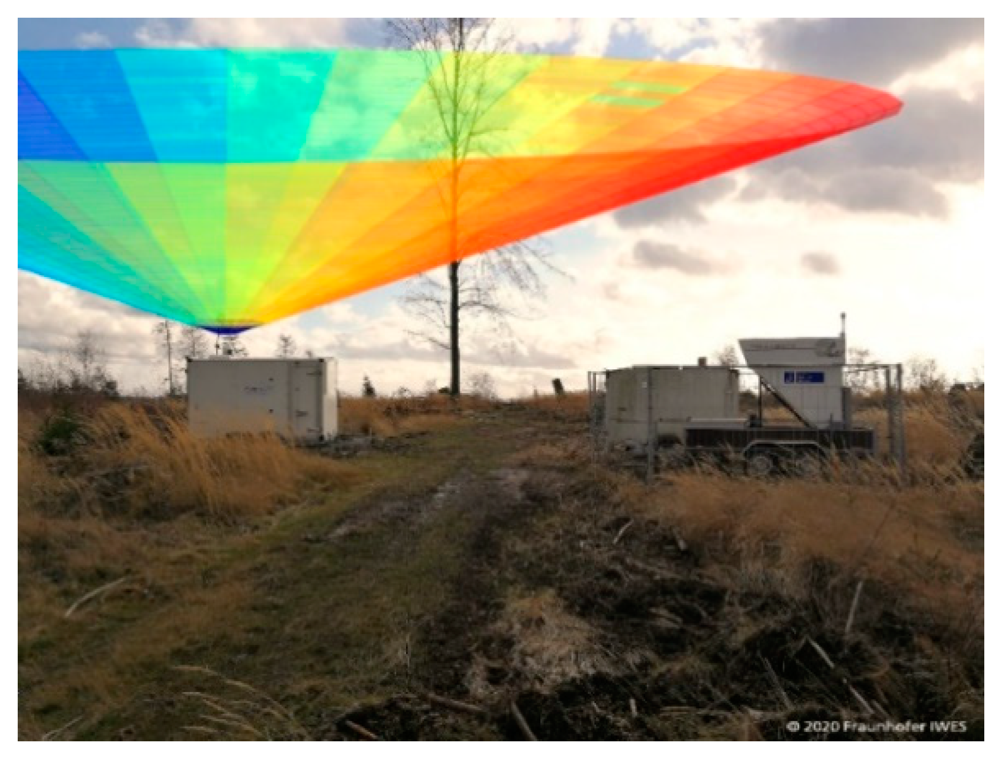
2.1.1. On-Site Measurements

The motivation for using a scanning lidar within a wind resource assessment campaign, as proposed here, is to map the flow over the terrain at the locations of interest in as much detail as possible. For this purpose, we use the functionality of a scanning lidar device, which allows us to freely select azimuth and elevation angles of the laser beam and thus also to implement planar scans. Typical planar scan approaches are the Plan Position Indicator (PPI), for which the elevation angle is kept constant and the azimuth angle is varied from 0 to 360°, or the Range Height Indicator (RHI) defined by a varying elevation but constant azimuth angle. The complete scan is composed of a set of single line-of-sight (LOS) measurements, each defined by a specific azimuth and elevation angle. For pulsed wind lidars, different ranges are assessed simultaneously, so that PPI and RHI scans yield not only trajectories but actual planes. More details about scanning wind lidar technology and its use in the wind industry and wind energy research so far are found e.g., in [11,12,13,14].
For our methodology, we have selected a PPI scan approach, whereby the scanning lidar device is placed in such a way that a relevant part of the site can be covered. Ideally, this is the center of the site, and all planned future wind turbine locations are within the range of the scanning device. This may mean, in particular, the turbine positions at hub height—which however might not be known at the time the measurement campaign is conducted—or the height range that is relevant for the validation of the flow models (typically 50–200 m), respectively. Another approach could be to focus on areas that are supposed to be challenging for the applied flow models. When applying a PPI scan with constant non-zero elevation angle, measurement heights of the scanning lidar increase with range—this peculiarity of the measurement approach will be taken up again in the discussion of the results.
Particularly in complex terrain, obstacles of various kinds (including orographic site characteristics and vegetation) can create blind spots to the scan. Placing the device at some elevation may help to overcome the issue. A hard-target mapping and analysis is used to locate obstacles and optimize the scan pattern. In some cases, especially for larger sites and sites with a greater number of wind turbines planned, respectively, it may be recommended to use more than one scanning lidar device but otherwise apply the procedure in exactly the same way.
For a single LOS, the scanning lidar device records the radial wind speed:
v L O S ( r , θ , ϕ ) = v ( r , θ , ϕ ) · n ^ ( θ , ϕ ) ,  
i.e., the three-dimensional wind vector v = ( v x ,   v y ,   v z ) , typically expressed in Cartesian coordinates, is translated into spherical polar coordinates and multiplied with the unit vector that defines the particular LOS direction. Here, θ is the azimuth angle, ϕ the elevation angle and r the range or distance to the device. The actual velocity retrieved by the lidar at a certain radial location represents a spatio-temporal convolution of the instantaneous line-of-sight velocity field, with this depending on the explicit lidar acquisition process and scanning parameters [15].
The devices that are suitable for our application, requiring in particular a sufficient range of one to several kilometers, are typically pulsed lidars. As already mentioned above, pulsed lidars come along with the benefit of providing recordings for several range gates r j along a specific LOS i simultaneously, defining a measurement grid v L O S ,   i ( r j , θ i , ϕ ) for a PPI scan with a fixed elevation angle ϕ = const .
Typically, and especially if the scanning lidar device is not placed on a significant elevation at the site, ϕ is not chosen to be zero ( ϕ > 0 ), which leads to the scan not forming a surface but a cone. Care should be taken to ensure that ϕ is as small as possible since large scan elevation angles can lead to higher uncertainties due to a higher contamination of the LOS projected wind speed by vertical components. Previous studies have suggested to consider 20° as upper threshold for ϕ when setting up a PPI scan [16,17]. In other studies, an even smaller value is recommended, which however is often not feasible particularly in complex terrain.
Figure 1 illustrates the measurement setup with a PPI scan by a scanning wind lidar device covering the site of interest. This areal measurement is supplemented by a reference measurement at one point, which can be realized by a vertically profiling lidar or sodar device or a met mast with several height levels, and which provides recordings of reference (horizontal) wind speed, direction and wind shear in terms of the wind shear exponent (see details later). The wind shear exponent is used here as a proxy for atmospheric stability, which is rather a pragmatic than optimal choice. These data are required for the merge of measured and numerical data which is described in detail in Section 2.1.3. From a practical point of view, the reference measurement can be identical to the main measurement required by TG 6 [6]. If the scanning lidar measurement is carried out after the end of this activity for a retrospective reduction of the WRA uncertainties, however, an additional reference measurement needs to be executed to provide the input data to the proposed methodology.

2.1.2. Wind Flow Simulation and Projection of Numerical Data

A numerical micro-scale wind flow model describes the spatial wind distribution by solving a fluid mechanics equation system on a predefined grid in a domain over the site, using physical parametrization. As input, the user needs to provide terrain maps (elevation, roughness and land-use) and boundary conditions (e.g., input wind speed, wind direction and stability). In a WRA study, the output of the wind flow models is used to spatially transfer the measured wind conditions from the reference instrument location to the WT locations. This is done by applying speed-up factors that account for topographical effects. A simplified model setup can be based on a pre-defined standard configuration with some wind direction sectors as input and stability factors (if reference measurements provide these) that can be chosen depending on the measured on-site wind conditions.
The most general output of a numerical wind flow simulation is a three-dimensional wind field, i.e., a three-dimensional wind vector for each point of the (again three-dimensional) simulation grid. In order to compare this output with the measurements of a single scanning lidar as described in Section 2.1.1, we project the numerical data onto the measurement grid v L O S ,   i ( r j , θ i , ϕ ) . This again requires a coordinate transformation from typically Cartesian to spherical polar coordinates and the consideration of the specific unit vectors that define the configured PPI scan. The projection provides the data matrix ( v L O S ,   i j ) s i m . which is in the next step compared to ( v L O S ,   i j ) m e a s . obtained directly from the scanning lidar measurements. This comparison is done for a specific wind direction φ and atmospheric stability as covered by the numerical simulations. Wind speeds are typically not varied for the simulations, which is why they do not represent an additional input parameter here. This assumption is supported by a dimensional analysis based on Monin-Obukhov similarity theory (MOST). The scaling behavior has been re-evaluated recently in [18,19]. That reduced the simulation matrix considerably which has been shown in [20] in case of meso-micro coupling using multiple meso-scale points that overlap with the micro-scale domain. Wind shear, as a proxy for atmospheric stability, is expressed by the power law shear exponent α which can also be derived from the reference measurement covering at least two measurement heights according to:
v h 2 = v h 1 · ( h 2 / h 1 ) α
where h 1 and h 2 are the two measurement heights and v h 1 , v h 2 the respective horizontal wind speed values. It should be noted that the choice of using the wind shear exponent as a proxy for atmospheric stability is generally accurate only in case of flat homogenous terrain without either forest or variation in land-use. Even if these conditions are not met for our study, using this proxy has a merit since we are considering it in relative terms with respect to neutral conditions while everything else is fixed. That is why we see it as a pragmatic and here still sufficient choice. A more advanced but still simple method is introduced in [21] combining the shear exponent with the turbulence intensity as another proxy for atmospheric stability.

2.1.3. Calibration of Numerical Flow Data

The measurement data are processed by applying a quality filter. A specific filter we have selected for our application is described in Appendix A. The filtered valid measurement data is then averaged to 30-min block averages. The averaged data matrices are each assigned a reference wind speed v h o r ,   r e f , direction φ r e f and wind shear exponent value α r e f that are derived from the simultaneous reference measurements. Values of φ r e f and α r e f are binned, i.e., rounded to some discrete values that define the respective bins, so that they are comparable to the input parameters of the numerical simulations.
Measured and simulated data matrices are now grouped according to these two parameters but still have different reference wind speeds in the majority of cases, namely when the measured reference wind speed does not correspond to the usually constant input wind speed used in the simulations. To eliminate this discrepancy, we carry out a normalization of the data matrices assuming that such a manipulation does not affect the characteristics of the wind flow. A straightforward normalization method is to divide both ( v L O S ,   i j ) m e a s . and ( v L O S ,   i j ) s i m . by the corresponding value of the outermost grid point, i.e., r = r m a x , along the mean wind direction φ r e f . This gives:
( v L O S ,   i j ) m e a s . / n o r m . = ( v L O S ,   i j ) m e a s . ( v L O S ,   i = ^ φ r e f ,   j = ^ r m a x ) m e a s .
( v L O S ,   i j ) s i m . / n o r m . = ( v L O S ,   i j ) s i m . ( v L O S ,   i = ^ φ r e f ,   j = ^ r m a x ) s i m .
After this normalization the measured and simulated data matrices of radial wind speeds can be correlated and deviations can be assessed. We call this a calibration because the results can be used to assess and quantify a model uncertainty which is a highly relevant input to the WRA evaluation. For this article, the deviations ( Δ v L O S ,   i j ) are assessed according to:
( Δ v L O S ,   i j ) = [ ( v L O S ,   i j ) s i m . / n o r m . ( v L O S ,   i j ) m e a s . / n o r m . ] / ( v L O S ,   i j ) m e a s . / n o r m .

2.2. Demonstration Study

The methodology described in the previous subsection is demonstrated by means of an example study, details of which are given in this subsection. In Section 2.2.1 we describe the site under investigation, in Section 2.2.2 the used measurement technologies and the measurements carried out, and in Section 2.2.3 the applied flow modelling with the two Computational Fluid Dynamics (CFD) models run for the site. Results of the study are presented and discussed in the following sections.

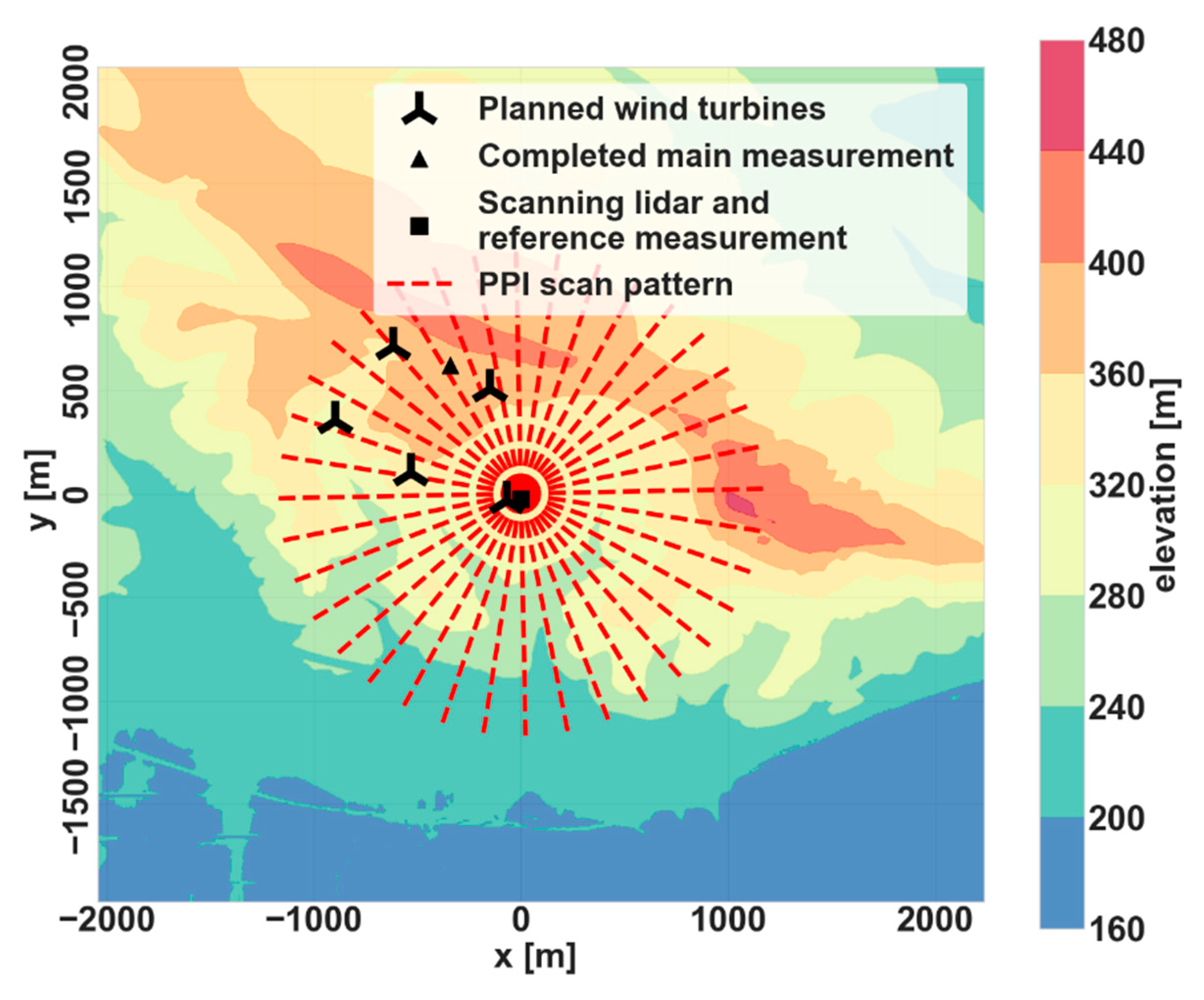
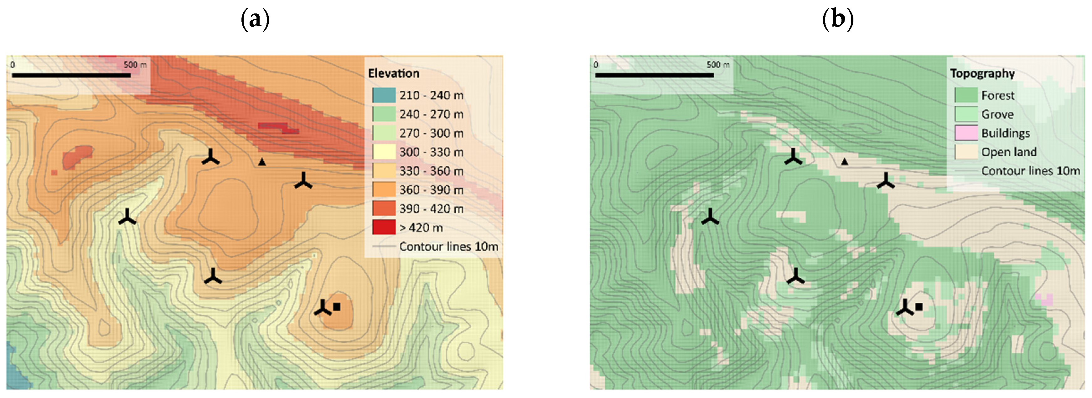
2.2.1. Description of Site

The site studied for this article lies in the municipality of Herleshausen in the state of Hesse (Germany) close to the border of Thuringia and is characterized as moderately complex dominated by forest. In the considered scenario, five wind turbines (with a hub height of 161 m each) are planned in the wind farm Herleshausen on and around a hill at heights between 300 and 400 m above mean sea level, as shown in Figure 2 together with the prevailing land-use type and orography. Elevations between the wind turbine locations planned in this scenario vary up to 50 m, leading to significant speed-up effects and posing a challenge for any wind flow model. For a specification of land-use types see additionally Table 1.

2.2.2. Used Measurements

A TG 6-compliant wind measurement with a vertically profiling wind lidar was carried out at the site already in 2015/16. However, as our study was only conducted subsequently, these measurements could not be used as direct reference measurements. For this reason, we have installed a supplementary sodar device, as shown in Figure 1 and Figure 2, that provided reference measurements of horizontal wind speed and direction (both at 120 m height) and the wind shear exponent (derived from the measurements at 60 m and 120 m) to the wind flow mapping of the scanning lidar and the flow modelling. The installed device is a Doppler miniSoDAR System by Atmospheric Systems Corporation (Boulder, CO, USA) configured to measure at 16 heights between 30 m and 180 m.
The scanning lidar device that was deployed at the site is a Galion 4000 [22], a long-range pulsed Doppler wind lidar and Wood Group product. In optimal conditions, it provides wind measurements in a distance range of up to 4000 m, starting at 80 m, with up to 130 sequential range gates of 30 m each. The laser’s shooting frequency is 100 Hz and the data sampling rate up to 2 Hz, depending on the specific instrument settings configured. The instrument has an all-sky scanning capability allowing e.g., for a PPI scan strategy as pursued in this study. For the detailed settings selected during our campaign, see Table 2.
The two devices were installed next to each other, see Figure 3, at a location that was identified as optimal in terms of the device’s clear view and coverage of the measurements. From this position, next to the planned turbine location WT3, the scanning lidar beams in the configured PPI scan could reach four of the total five planned wind turbine locations in the given scenario. Details of the configured scan are given in Table 2. Measurements with this scan strategy were run for a total period of about four weeks in fall 2019 and winter 2020 (details are also given in Table 2) with an alternative strategy not discussed here pursued in the period in between.

2.2.3. Applied Flow Modelling

In this study, two micro-scale CFD models have been used, FIWind and FITNAH. Fraunhofer IWES Wind Simulation Environment (FIWind) is an in-house tool developed by Fraunhofer IWES based on OpenFOAM. The version used in this work is based on OpenFOAM-5. The second model is Flow over Irregular Terrain with Natural and Anthropogenic Heat Sources (FITNAH) [23,24] which is a meso-scale type model adapted and advanced by GEO-NET for wind mapping and resource assessment.
Both the above mentioned CFD models are steady-state Reynolds-Averaged Navier-Stokes (RANS) models. The flow is considered incompressible under the Boussinesq approximation. Despite the similarities in the core physics, there are several significant differences between the models: for the FIWind setup, an Atmospheric Surface Layer (ASL) model has been used based on [25], which means that the Coriolis force is ignored. FITNAH, on the other side, includes an Atmospheric Boundary Layer (ABL) model which—in contrast to FIWind—has the capability to predict veer. Another major difference is the type of mesh used: unlike FITNAH, which is a structured code, FIWind can use an unstructured mesh. In FIWind a cylindrical domain with horizontally uniform grid is used for all wind directions whereas in FITNAH a rectangular domain with a horizontally uniform grid is used. Both models include a canopy model for forest modelling representing the canopy by extra source terms in the momentum and turbulence equations. The land-use map as per Figure 2 has been used and the roughness values and forest parameters in Table 1. The plant area density profiles for forest and grove type follow [26]. More details about the general FIWind formulation can be found in [25,27].
In order to have a good basis for a comparison between the two models, the differences in the model setups are kept as small as possible. The same grid resolution of 25 m has been used with the same land-use and forest parametrization, thus the same roughness and plant area density profiles. Only neutral conditions have been considered with 36 simulated wind directions in FIWind and 12 directions in FITNAH, both uniformly distributed. The difference in the number of modelled wind direction sectors is mainly due to limitations in computational resources. Details of the model setups are summarized in Table 3. As mentioned before, only one reference wind speed is necessary since the velocity field can be scaled later. Only neutral stratification has been considered to eliminate the uncertainty associated with the choice of thermal parameters. Moreover, there are some differences in the implementation of the thermal solvers in the two codes, which is however eliminated by modelling neutral conditions only.

3. Results

First, in Section 3.1, we describe how the data from the entire measurement campaign was sorted and assigned to individual flow cases. In Section 3.2, we investigate a single flow situation that corresponds to one 30-min dataset, and in Section 3.3 we present a statistical analysis of four selected flow cases.

3.1. Data Coverage

After processing the data, a two-dimensional capture matrix, summarizing the distribution of the recorded data with respect to the reference parameters, was derived to map the coverage of individual flow cases. The dimensions of the capture matrix are reference wind direction φ r e f and vertical wind shear exponent α r e f as obtained from the on-site reference data, i.e., the sodar recordings in our case. The reference wind direction is measured at 120 m above the sodar instrument, and the values α r e f are derived by fitting a power-law profile to the wind speed measurements at the two heights 120 m and 60 m, as described above. The data are then binned according to wind direction bins / intervals of 30° and wind shear exponent bins/intervals of 0.2, resulting in the matrix shown in Figure 4. The two-dimensional data distribution is investigated in order to select the most relevant flow cases. For our study, these are cases with an inflow wind direction from the sectors around 210° and 240° and a wind shear exponent in the range between 0.1 and 0.5, i.e., in the bins around 0.2 and 0.4.
In principle, all flow cases that are considered as relevant based on the data from the main measurement and a suitable long-term reference dataset should be covered by the additional measurement involving the scanning lidar with a sufficient number of samples. In our study, this could not be realized to full extent due to the limited and rather short length of the campaign. This is why we focus on four flow cases only to demonstrate the principle of capability of the proposed methodology.

3.2. Single Flow Situation

For a single flow situation, we consider an individual 30-min dataset comprising the reference sodar measurements, the corresponding averaged PPI scan obtained by the scanning lidar, and the projected flow simulations by the two numerical models with boundary conditions as defined by the reference measurements. The flow situation we selected for the purpose of demonstration was recorded on 12 February 2020 01:30 UTC and is characterized by a reference wind direction of φ r e f = 240 ° and a wind shear exponent of α r e f = 0.4 .
Measured and simulated data matrices ( v L O S ,   i j ) m e a s . / n o r m . and ( v L O S ,   i j ) s i m . / n o r m . as well as their deviations ( Δ v L O S ,   i j ) , presented as contour plots over the underlying terrain, are shown in Figure 5. The majority of identified deviations follows the terrain with most of them being related to speed-up effects due to the hills, as in the south-west of the deployed scanning lidar device. When the wind approaches from south-west, it speeds up right before the hill on which the device is installed. This speed-up is overpredicted by both models but being more visible in the FITNAH results. The grey areas indicate a mismatch between the scanning lidar’s and the virtual lidar’s blind region, i.e., the corresponding region (in the measurement or the projected simulation data, respectively) where the LOS direction is perpendicular to the wind direction. For this region we expect a higher uncertainty of the scanning lidar measurements due to the measurement principle and geometry, respectively, as further detailed in Appendix B. But the width of the grey region also increases as the simulated wind direction deviates from the actual prevailing wind direction. For the presented flow simulation the input direction (at 120 m) has been 229° and 244° for FITNAH and FIWind, respectively, where the larger mismatch of FITNAH is solely due to the smaller number of simulated wind direction sectors.

3.3. Selected Flow Cases

As already mentioned above, we have further selected four different flow cases, which are predominant in the capture matrix for the site conditions. These are the wind direction sectors around 210° and 240° combined with the wind shear exponent bins around 0.2 and 0.4, resulting in the four aforementioned cases. In this work, the cases with shear exponent 0.2 are considered more neutral compared to 0.4. Although 0.2 shear exponent is higher than the classical 1/7 shear exponent for neutral conditions, it is more reasonable in this case since we have a complex terrain with heterogeneous forest. This topic has been discussed in an early technical note [28] and more recently in [29]. In both articles, researchers showed the variation in shear exponent based on measurements with respect to terrain complexity and stability. In many of these observations, the neutral conditions have a shear exponent around 0.2 with a wide scatter.
All recorded individual flow situations, i.e., processed 30 min datasets of scanning lidar measurements, with reference wind conditions lying in these wind direction and shear exponent bins were collected and averaged to give the contour plots in Figure 6 ( φ r e f = 210°) and Figure 7 ( φ r e f = 240°), panels (a) and (b). As in Figure 5, we compare measured and simulated LOS data, considering for each wind direction sector (around 210° and 240°, respectively) two shear exponent bins covered by the measurement data. Simulated data remain the same since the input shear exponent or stability is not changed for the models and simulations. The comparisons with the corresponding measurement therefore show how well the simulations cover the different shear conditions. These comparisons in panels (d, e) and (g, h) are to be considered together with the contour plots in Figure 8 and Figure 9, respectively, which show the statistical uncertainties of the collected measurements. For this the standard error of the averaged PPI data is shown. Blind spots are clearly visible where obstacles have reduced the data availability. The statistical uncertainty has also been considered as lower threshold for the deviations shown in Figure 6 and Figure 7.
We can make the following observations:
-
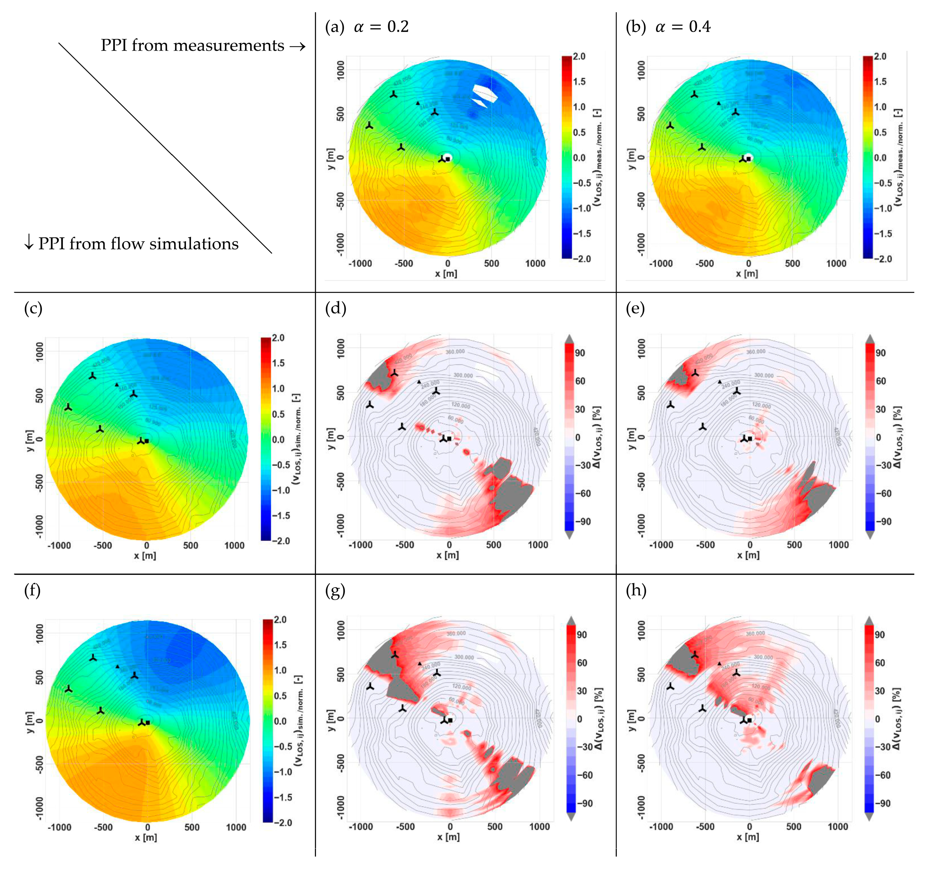
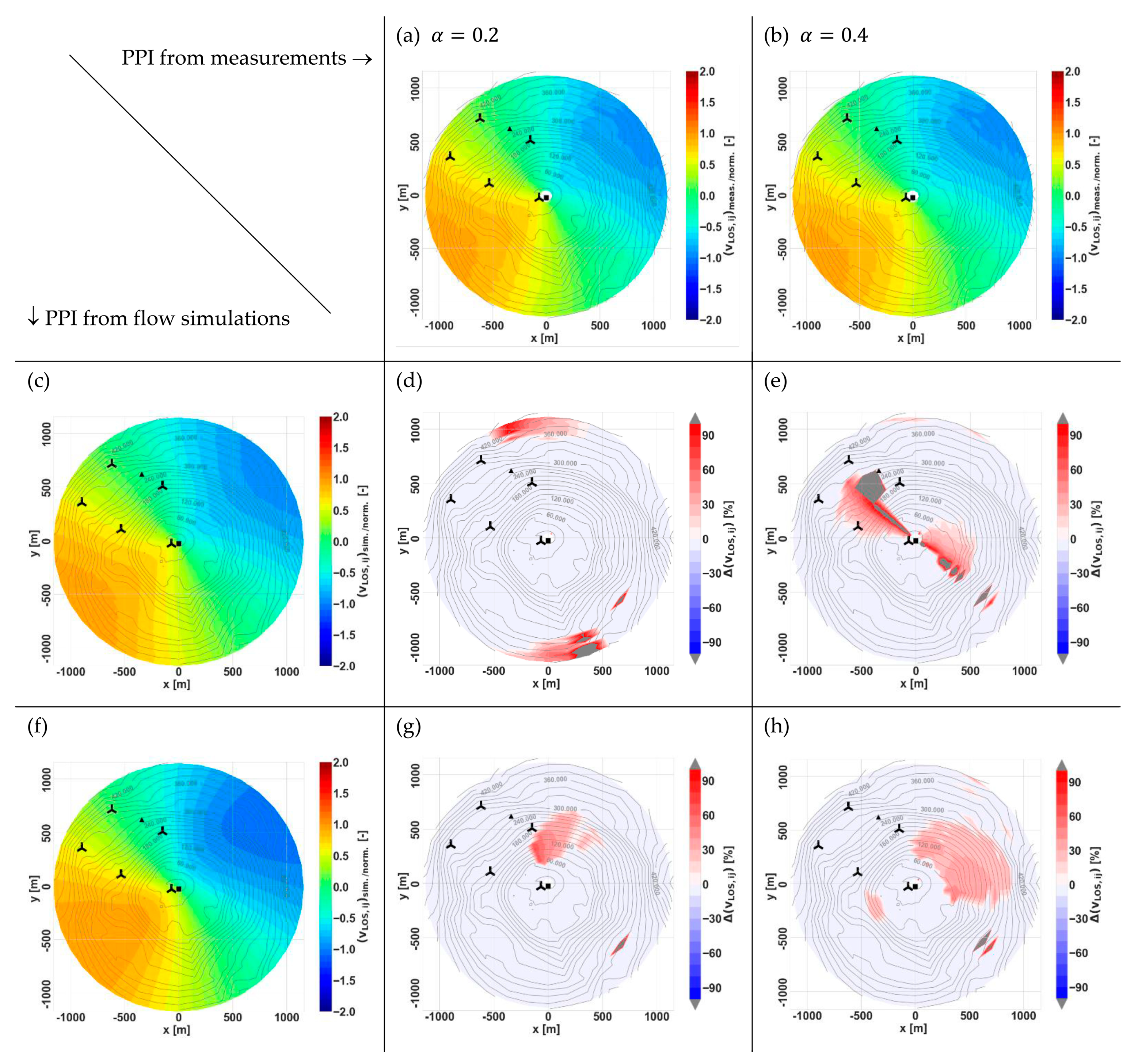
When comparing the contour plots for the individual flow situation in Figure 5 and the averaged flow cases in Figure 7, with the same wind direction sector (240°) studied here, it is obvious that any local inhomogeneities, which are seen in the single flow situation comparison and can be connected with the non-stationarity of the wind conditions, are now averaged out.
-
The conical gray patterns again indicate a misalignment of the measurements with the simulations—for the averaged flow cases, this misalignment is however in a similar order for the two models.
-
For both wind directions shown in Figure 6 and Figure 7, the absence of the veer, i.e., wind direction shear (or rotation of wind with increasing height), in FIWind is indicated in terms of the pronounced deviations of the simulation results to the measurements at the outer parts of the PPI contour plots, which correspond due to the conical shape of the scan to higher altitudes. The results for FITNAH do not show these deviations to this extent, which may be explained by the fact that the veer is covered by the model as pointed out in Section 2.2.3.
-
Furthermore, we observe an over-speeding around the hill on which the scanning lidar was placed for the FITNAH results. This effect is reduced for the case with the lower shear exponent α r e f = 0.2 . Since the same terrain data is used as input to FITNAH and FIWind, we assume this over-speeding to be due to the other boundary conditions, i.e., the considered wind profile and again the reference wind direction.

4. Discussion

In this section we discuss the obtained results by addressing the following points: first, we discuss the insights gained and the potential of the introduced methodology; then we look at its limitations; and finally, we explain how the methodology can be applied within the framework of a WRA study and thus achieve the set goal of advancing a WRA in complex terrain with scanning lidar measurements.

4.1. Potential of the Found Results

The objective for the introduction of the scanning lidar measurements has been to detect deviations of the numerical data or the models, respectively, from the measurements that could lead to an error in the estimated wind potential following the standard WRA procedures. Indeed, the results presented in Section 3 indicate that projecting numerical flow simulations on the scanning lidar geometry and comparing these data to the real measurements by the deployed scanning lidar device can reveal large deviations. Some of these deviations are due to a sensitivity to the setup of the numerical model and particularly the number of simulated wind direction sectors. Such resolution effects need to be carefully considered when interpreting this kind of calibration and deriving uncertainties from it. But, once this is controlled, the deviation maps can provide useful insight in areas for which the speed-up effects of the flow are not represented correctly or in the missing of certain physical effects in the one or the other model. The latter was indicated for the example of veer that is not included in one of the models. Wind shear and veer effects are covered by the scanning lidar measurements as the implemented PPI scan describes a cone (with an elevation angle ϕ > 0 ) and thus cuts through the three-dimensional wind field at different heights depending on the range or distance from the instrument. For the observed effect we cannot say with absolute certainty that it is indeed veer—the PPI scan only gives a cone-shaped section through the three-dimensional wind field, so it could be any other effects leading to the same projection.

4.2. Limitations and Challenges to the Introduced Methodology

As already mentioned, some deviations result from the fact that the simulated and measured wind directions and shear exponents only match to a limited extent. These deviations can be reduced, in principle, by reducing the size of the bins, i.e., increasing the resolution for the comparison. However, this is not always possible due to limited computational resources, especially having the application of the procedure in a standard WRA study in mind. The limited resolution of reference wind directions could be taken into account by weighting the individual flow situations averaged in a bin, which was however not done here. The respective resolution with the size of the bins must be taken into account in the final assessment of uncertainties to be derived based on the proposed procedure, which is discussed in the last paragraph of this section. Moreover, only one stability condition was considered here, namely neutral. For the measurements it is, however, difficult to isolate purely neutral conditions, which results in some uncertainty regarding the interpretation of the results. The measurements could be filtered and both turbulence intensity and shear exponent can be used as proxy for thermal stability. In such complex terrain with forested patches, it would be actually more accurate to use turbulence intensity for each stability class in relative terms with respect to neutral conditions.
Another limitation exists in the assumed stationarity. The measurements are averaged, first over 30 min periods and then over all individual situations found for a particular flow case, to be comparable to the steady-state simulations. Depending on the stratification of the atmosphere and the prevailing turbulence length scales, the initial averaging may not always be sufficient to get rid of the local inhomogeneities as it is seen in the studied flow situation in Section 3.2. Remaining inhomogeneities are mixed with terrain-dependent deficiencies of the models. The further clustering to flow cases helps to separate the latter whereby the corresponding bin sizes are to be determined with care. For a more thorough handling of stationarity, the data may be first filtered to exclude mesoscale fluctuations following e.g., the procedure in [30] before a more quantitative method is applied to check the stationarity of the statistics of interest (cf. for instance [31]). Studying the statistical uncertainty of the averaged measurements, in terms of the standard error as shown in Figure 7 and Figure 9, may give a hint on the effectiveness of the averaging even without a more in-depth investigation of stationarity.
The applied normalization also requires particular attention. In order to bring the simulations and measurements to a comparable state, we removed the information of the boundary wind speed by applying a corresponding normalization. For this we have assumed that the wind field distribution over the terrain is independent from the boundary wind speed itself but depends only on the terrain and atmospheric stability. One of the factors which may challenge this assumption is the steepness of the terrain. For high steepness, it is common to observe flow separation, resulting in different distributions of the wind field for low and high wind speeds. Other effects that may play a role here and be necessary to be taken into account are those related to the Froude number or the buoyancy of the capping inversion which may lead to flow modifications such as gravity waves. A more refined normalization procedure may take care of this effect.
For an assessment of the uncertainties related to the methodology, we should consider the following further aspects. First, both the simulated and the measured data are subject to discretization—for the simulations defined by the numerical grid, for the scanning lidar measurement by the chosen azimuth and range gate resolution. Due to the different initial geometries, there may be uncertainties in the projection of the numerical data. The measurement data are, further, characterized by a finite measurement volume that extends only along the LOS for our application. For a pulsed lidar, we have a constant sampling volume for all range gates and corresponding constant range resolution. A third aspect to consider is the uncertainty of the reconstructed wind speed with respect to azimuth and wind direction. Scanned components that are perpendicular to the mean wind direction vanish, so that the areas in the vicinity are characterized by a higher degree of uncertainty. A simplified analytical investigation of these geometric uncertainties is summarized in Appendix B. Finally, the uncertainty assessment has to be applied on a wide range of atmospheric conditions in order to unlock the full potential of the proposed methodology.

4.3. Application within WRA Study

The purpose of the introduced methodology is to calibrate the output data of a numerical flow model with the data from a scanning lidar measurement, and with this potentially reducing the uncertainties of a wind resource estimate. In the most general metrological definition, calibration means the comparison of the values measured by a so-called device under test, which are here the flow models, with those of a calibration standard of known accuracy [32]. The calibration standard is in our case the prepared set of radial wind speed measurements by the scanning lidar. With a suitable verification procedure (not further discussed in this article) we can make sure that the accuracy of our calibration standard is known, which does not necessarily mean that the associated uncertainties are particularly low. However, because we work with direct measurements of the radial velocities and do not apply any further reconstruction methods to the measurement data, we can actually assume relatively low uncertainties even in complex terrain.
The outcome of the comparison that comprises the calibration can result in one of the following conclusions:
-
no significant errors are found for the device under test,
-
a significant error is found but no adjustment is considered, or
-
an adjustment is undertaken to correct the error to some acceptable level.
Often the term calibration is only used for this latter adjustment which however is not fully correct according to the strict metrological definition. Of particular practical importance is the accompanying quantification of uncertainty: an estimated uncertainty can be related both to the level of significance and acceptance referred to in the evaluation of the comparison. An adjustment (in our case, of the flow model or its settings and boundary conditions) may help to reduce the uncertainties but not beyond the significance level that is defined by the uncertainty of the scanning lidar measurements used for calibration and the limitations of the undertaken comparison as e.g., the mentioned limited resolutions.
It is a legitimate question whether enough significance remains in the end for the results of this calibration to have a relevant impact on the wind resource estimates within a WRA study. Although we have not yet been able to show this in the present study (mainly due to the limited period and coverage of the undertaken measurements), we assume that this is the case. The introduced methodology offers an opportunity to quantify the uncertainty of the applied flow models and means a paradigm shift from the usual way of dealing with the uncertainties of flow model simulations. Determining the uncertainties via this type of calibration and no longer just roughly estimating them does not necessarily mean that the determined values in the first step are lower. But in the long term, we think, this approach offers a basis for using and developing flow models in a more targeted way and thus achieving higher-quality wind resource estimates.

5. Conclusions

In this article, we have shown how a single additional scanning lidar device can be used to calibrate the output data of a numerical flow model and with this potentially reduce the uncertainties of the final wind resource estimate. This in particular provides a large opportunity when considering flow patterns and not just single points in different ambient conditions. In detail, the methodology consists of mapping the characteristic flow over the site and terrain of interest and comparing the flow model simulations, which are an integral part of the standard wind resource assessment, to these measurements. By using the scanning lidar measurements obtained from a PPI scan as they are and projecting the flow model simulations onto the geometry defined by this scan, measurement uncertainties can be kept low and the significance of the comparison is maximized.
The methodology was demonstrated based on the data of a measurement campaign for the site of Herleshausen in central Germany characterized by moderately complex terrain. The simulations of two different flow models, FIWind and FITNAH, were compared with the obtained measurements. Before, the measurement data were filtered based on a combined range-CNR filter, allowing us to reproduce a large amount of the flow over the considered terrain. The considered flow models tend to overestimate at least specific points of the projected and scaled wind fields by up to 90%. A tuning of the models may be a natural further step of the methodology but was not within the scope of the presented analysis.
Although this study did not comprise a complete wind resource assessment, the results found demonstrate the potential of the methodology. We can conclude that the use of scanning lidar technology in WRA studies offers a new and promising opportunity to quantify the uncertainty of the applied flow models, which can otherwise only be estimated very roughly. The application of the technology is targeted in such a way that additional costs are kept as low as possible and an optimal intersection between added value and additional expenses is found.

Author Contributions

Conceptualization, J.G. and A.P.; provision of simulation and measurement data, A.P. and H.K. and L.S. and C.W.; data analysis, A.P.; writing—original draft preparation, J.G. and A.P.; writing—review and editing, all; uncertainty modelling input—P.J.M.; funding acquisition, J.G. and J.B. All authors have read and agreed to the published version of the manuscript.

Funding

The presented results have been produced within the framework of the EWiNo project funded by the Federal Ministry for the Economic Affairs and Energy on the basis of the decision by the German Bundestag under the grant number 0324225A/B. FIWind simulations were performed at the high-performance computing cluster EDDY, located at the University of Oldenburg (Germany), and funded by the Federal Ministry for Economic Affairs and Energy under grant number 0324005.

Data Availability Statement

Not applicable.

Acknowledgments

We thank the wind farm developer ENERTRAG for giving access to the site to carry out the measurements campaign as well as providing the detailed scenario for this study.

Conflicts of Interest

The authors declare no conflict of interest.

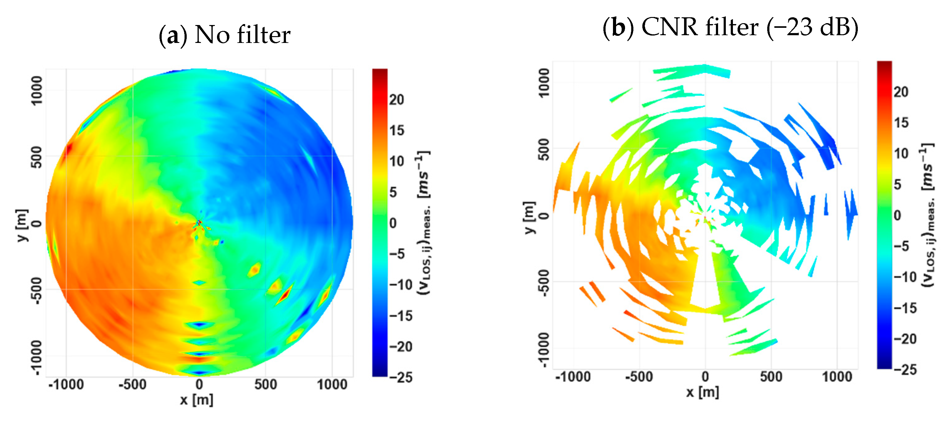
Appendix A. Filter Applied to Scanning Lidar Data

All scanning lidar data that were evaluated for this study were pre-processed by applying a combined CNR and range filter which is described in the following and illustrated in Figure A1. Unfiltered data of a wind lidar, as shown in Figure A1a, often contain artefacts that are generated by particularly high or low backscatter due to e.g., obstacles/hard targets or low aerosol concentrations. A standard approach is to consider only recordings with a certain signal strength and e.g., a carrier-to-noise ratio (CNR) within a defined range. Lower CNR thresholds, as also shown in Figure A1b, are very common and limit among others the maximum measurement height of a vertically profiling lidar or the range of a more or less horizontally scanning lidar, respectively. But upper thresholds are sometimes applied as well to exclude situations with unusually high backscatter.
Figure A1b illustrates that a too conservatively chosen threshold value for a CNR filter, here 23   dB , may exclude a large amount of data and also data regions that show no artefact. For this reason, it may be advisable for some applications to consider also other types of filters. For this study we have used a simplified filter (compared to approaches seen by [33,34]) that improves availability by combining a CNR filter with a lower threshold value of 30   dB with a range filter. This additional step removes peaks along the line of sight based on the expected spread of radial wind speeds. Range filtering is used extensively in image processing, as described in [35], and already applied to long-range wind lidar data in [36]. For this type of filter, a threshold value is considered which is depending on the azimuth angle θ i and corresponds to the maximum recorded dispersion σ of the radial wind speeds along this direction, i.e.,:
Th i = max ( σ i ,   r = 0 ,   ,   σ i ,   r = r m a x ) .
As shown in Figure A1c, this range filter performs quite well in deleting obvious artefact regions in the exemplary PPI scan. In combination with a reduced CNR filter—see Figure A1d—it is possible to remove all unwanted data points without losing too much data.
Figure A1. Illustration of different filters for the processing of the radial wind speed measurements of the scanning lidar; for explanations see text.
Energies 14 03280 g0a1aEnergies 14 03280 g0a1b

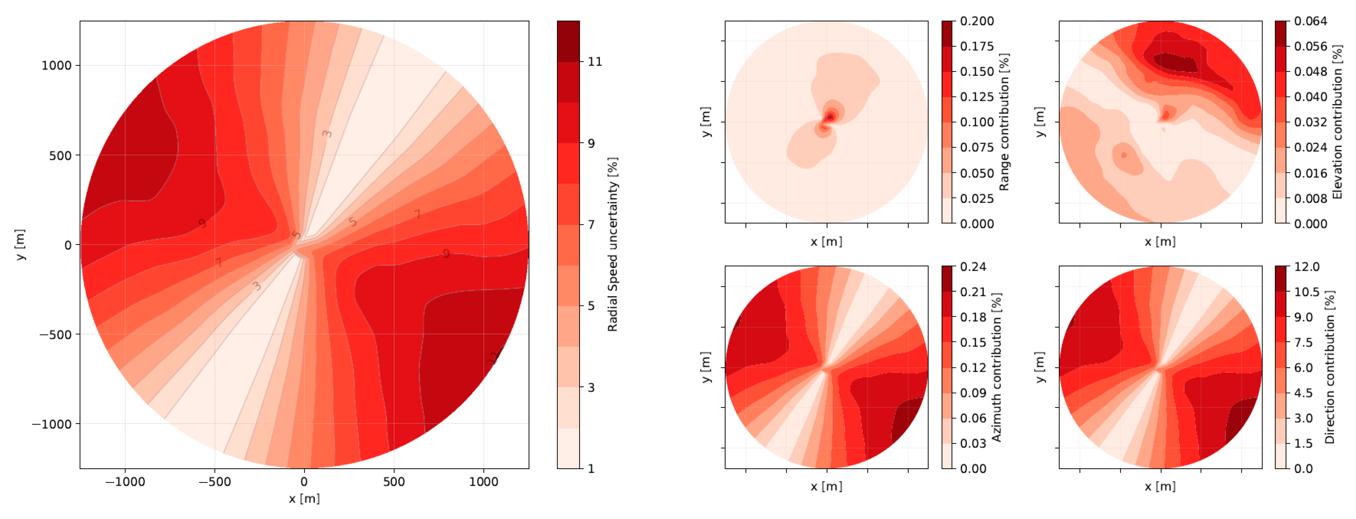
Appendix B. Scanning Lidar Uncertainty Modelling

The PPI scan data of a scanning lidar device, as we have used them for this study, are composed of individual LOS measurements each defined by a well-defined geometry. The geometric parameters—i.e., explicitly the range r , azimuth and elevation, θ and ϕ , respectively—are to be considered together with an uncertainty each that propagates through to the measured LOS wind speed. This propagation can be comprehended analytically as it is outlined in [37].
Figure A2 shows the derived contributions for one of the flow cases we have studied for the Herleshausen site—with a reference wind direction of φ = 210 ° and wind shear exponent of α = 0.2 . The underlying terrain was used as input as for the numerical flow simulations described above, and the fixed elevation angle of the PPI scan was set to 20 ° as in the real measurements. As reference wind speed we have considered 1 (normalized), and uncertainty contributions are given as percentage values with reference to this. For azimuth and elevation we have considered an input uncertainty of 0.1 ° , respectively, for the range an uncertainty of 1   m , and for the measured wind speed an uncertainty of 1 % .
Comparing the three uncertainty contributions from range, elevation and azimuth, the contribution of the last of these three is the largest with a greater impact for LOS directions perpendicular to the prevailing wind direction. The elevation uncertainty is clearly determined by the terrain and has its largest contribution where the azimuth uncertainty vanishes for the considered flow case.
As an extension of the model developed in [37], we have added another contribution due to the uncertainty in reference wind direction. This uncertainty contribution may be caused both by a measurement uncertainty of the recorded reference wind direction and the misalignment of wind directions from numerical models and measurements for the comparison and derivation of deviations. This direction contribution, also shown in Figure A2, follows the same pattern as the azimuth contribution but with significantly larger values when considering an input wind direction uncertainty of 5 ° as suggested for this study. Combining all individual contributions in an overall geometric uncertainty, the direction uncertainty is clearly dominant. This emphasizes the necessity for reducing this impact by e.g., introducing a finer binning for the comparisons of numerical and measured data and with this improving the matching of observed and simulated wind directions.
Figure A2. Analytically derived uncertainty contributions for LOS measurements of PPI scan—here for the flow case defined by φ = 210 ° and α = 0.2 . Uncertainties are given as percentage values with respect to a reference wind speed normalized to 1.
Energies 14 03280 g0a2

References

  1. BMWi (German Federal Ministry of Economic Affair and Energy) Renewable Energy Sources Act (EEG 2017). Available online: https://www.bmwi.de/Redaktion/DE/Downloads/E/eeg-2017-gesetz-en.pdf?__blob=publicationFile&v=8 (accessed on 31 January 2021).
  2. Lee, J.C.Y.; Fields, J.M. An Overview of Wind Energy Production Prediction Bias, Losses, and Uncertainties. Wind Energy Sci. 2021. [Google Scholar] [CrossRef]
  3. Clifton, A.; Smith, A.; Fields, J.M. Wind Plant Preconstruction Energy Estimates: Current Practice and Opportunities; NREL/TP-5000-64735; National Renewable Energy Laboratory: Golden, CO, USA, 2016.
  4. Brower, M.C. Wind Resource Assessment: A Practical Guide to Developing a Wind Project; John Wiley & Sons, Inc.: Hoboken, NJ, USA, 2012. [Google Scholar] [CrossRef]
  5. MEASNET: Evaluation of Site-Specific Wind Conditions. Version 2. April 2016. Available online: https://www.measnet.com/wp-content/uploads/2016/05/Measnet_SiteAssessment_V2.0.pdf (accessed on 31 January 2021).
  6. FGW. TR 6—Bestimmung von Windpotenzial und Energieertrag; Revision 11; Fördergesellschaft Windenergie und andere Dezentrale Energien: Berlin, Germany, 2020. [Google Scholar]
  7. IEC. IEC CD 61400-15: Wind Energy Generation Systems—Part 15-1: Site Suitability Input Conditions for Wind Power Plants; Committee Draft (CD); IEC: Geneva, Switzerland, 2020. [Google Scholar]
  8. Tang, X.; Stoevesandt, B.; Fan, B.; Li, S.; Yang, Q.; Tayjasanant, T.; Sun, Y. An on-site measurement coupled CFD based approach for wind resource assessment over complex terrains. In Proceedings of the 2018 IEEE International Instrumentation and Measurement Technology Conference (I2MTC), Houston, TX, USA, 14–17 May 2018; pp. 1–6. [Google Scholar] [CrossRef]
  9. Saarnak, E.; Bergström, H.; Söderberg, S. Uncertainties Connected to Long-Term Correction of Wind Observations. Wind Eng. 2014, 38. [Google Scholar] [CrossRef]
  10. IEA Wind Expert Group Study on Recommended Practices 15. Ground-Based Vertically Profiling Remote Sensing for Wind Resource Assessment, First Edition. January 2013. Available online: https://community.ieawind.org/publications/rp (accessed on 31 January 2021).
  11. Vasiljevic, N.; Vignaroli, A.; Bechmann, A.; Wagner, R. Digitizing scanning lidar measurement campaign planning. Wind Energy Sci. 2020, 5, 73–87. [Google Scholar] [CrossRef] [Green Version]
  12. Vasiljevic, N.; Lea, G.; Courtney, M.; Cariou, J.-P.; Mann, J.; Mikkelsen, T. Long-Range WindScanner System. Remote Sens. 2016, 8, 896. [Google Scholar] [CrossRef] [Green Version]
  13. Wang, H.; Barthelmie, R.J.; Clifton, A.; Pryor, S.C. Wind measurements from arc scans with Doppler wind lidar. J. Atmos. Ocean. Technol. 2015, 32, 2024–2040. [Google Scholar] [CrossRef]
  14. Barkwith, A.; Collier, C.G. Lidar observations of flow variability over complex terrain. Meteorol. Appl. 2011, 18, 372–382. [Google Scholar] [CrossRef]
  15. Puccioni, M.; Iungo, G.V. Spectral correction of turbulent energy damping on wind lidar measurements due to spatial averaging. Atmos. Meas. Tech. 2021, 14, 1457–1474. [Google Scholar] [CrossRef]
  16. Drobinski, P.; Carlotti, P.; Redelsperger, J.-L.; Masson, V.; Banta, R.M.; Newsom, R.K. Numerical and Experimental Investigation of the Neutral Atmospheric Surface Layer. J. Atmos. Sci. 2007, 64, 137–156. [Google Scholar] [CrossRef]
  17. Pichugina, Y.L.; Tucker, S.C.; Banta, R.M.; Brewer, W.A.; Kelley, N.D.; Jonkman, B.J.; Newsom, R.K. Horizontal-Velocity and Variance Measurements in the Stable Boundary Layer Using Doppler Lidar: Sensitivity to Averaging Procedures. J. Atmos. Ocean. Technol. 2008, 25, 1307–1327. [Google Scholar] [CrossRef]
  18. van der Laan, M.P.; Andersen, S.J.; Réthoré, P.-E. Brief Communication: Wind-Speed-Independent Actuator Disk Control for Faster Annual Energy Production Calculations of Wind Farms Using Computational Fluid Dynamics. Wind Energy Sci. 2019, 4, 645–651. [Google Scholar] [CrossRef] [Green Version]
  19. van der Laan, M.P.; Andersen, S.J.; Kelly, M.; Baungaard, M.C. Fluid Scaling Laws of Idealized Wind Farm Simulations. J. Phys. Conf. Ser. 2020, 1618, 062018. [Google Scholar] [CrossRef]
  20. Buhr, R.; Kassem, H.; Steinfeld, G.; Alletto, M.; Witha, B.; Dörenkämper, M. A Multi-Point Meso–Micro Downscaling Method Including Atmospheric Stratification. Energies 2021, 14, 1191. [Google Scholar] [CrossRef]
  21. Svenningsen, L.; Slot, R.M.M.; Thøgersen, M.L. A novel method to quantify atmospheric stability. J. Phys. Conf. Ser. 2018, 1102, 012009. [Google Scholar] [CrossRef]
  22. Wood Galion Lidar Unit. Available online: https://www.woodplc.com/capabilities/digital-and-technology/software,-applications-and-analytics/galion-lidar-unit (accessed on 31 January 2021).
  23. Gross, G. The exploration of boundary layer phenomena using a nonhydrostatic mesoscale model. Meteorol. Z. 2002, 11, 295–302. [Google Scholar] [CrossRef]
  24. Gross, G.; Frey, T.; Trute, P. Die Anwendung numerischer Simulationsmodelle zur Berechnung der lokalen Windverhältnisse in komplexem Gelände. DEWI-Magazin 2002, 20, 28–36. [Google Scholar]
  25. Chang, C.-Y.; Schmidt, J.; Dörenkämper, M.; Stoevesandt, B. A Consistent Steady State CFD Simulation Method for Stratified Atmospheric Boundary Layer Flows. J. Wind Eng. Ind. Aerodyn. 2018, 172, 55–67. [Google Scholar] [CrossRef]
  26. Bonan, G.B.; Patton, E.G.; Harman, I.N.; Oleson, K.W.; Finnigan, J.J.; Lu, Y.; Burakowski, E.A. Modeling Canopy-Induced Turbulence in the Earth System: A Unified Parameterization of Turbulent Exchange within Plant Canopies and the Roughness Sublayer (CLM-Ml V0)’. Geosci. Model Dev. 2018, 11, 1467–1496. [Google Scholar] [CrossRef] [Green Version]
  27. Akbarzadeh, S.; Kassem, H.; Buhr, R.; Steinfeld, G.; Stoevesandt, B. Adjoint-Based Calibration of Inlet Boundary Condition for Atmospheric Computational Fluid Dynamics Solvers’. Wind Energy Sci. 2019, 4, 619–632. [Google Scholar] [CrossRef] [Green Version]
  28. Irwin, J.S. A Theoretical Variation of the Wind Profile Power-Law Exponent as a Function of Surface Roughness and Stability. Atmos. Environ. 1979, 13, 191–194. [Google Scholar] [CrossRef]
  29. Xu, C.; Hao, C.; Li, L.; Han, X.; Xue, F.; Sun, M.; Shen, W. Evaluation of the Power-Law Wind-Speed Extrapolation Method with Atmospheric Stability Classification Methods for Flows over Different Terrain Types. Appl. Sci. 2018, 8, 1429. [Google Scholar] [CrossRef] [Green Version]
  30. Lenschow, D.H.; Wulfmeyer, V.; Senff, C. Measuring second-through fourth-order moments in noisy data. J. Atmos. Ocean. Technol. 2000, 17, 1330–1347. [Google Scholar] [CrossRef]
  31. Foken, T.; Göockede, M.; Mauder, M.; Mahrt, L.; Amiro, B.; Munger, W. Post-field data quality control. In Handbook of Micrometeorology; Springer: Dordrecht, The Netherlands, 2014; pp. 181–208. [Google Scholar]
  32. JCGM 200:2012 International Vocabulary of Metrology—Basic and General Concepts and Associated Terms (VIM) 3rd Edition. Available online: https://www.bipm.org/utils/common/documents/jcgm/JCGM_200_2012.pdf (accessed on 31 January 2021).
  33. Beck, H.; Kühn, M. Dynamic Data Filtering of Long-Range Doppler LiDAR Wind Speed Measurements. Remote Sens. 2017, 9, 561. [Google Scholar] [CrossRef] [Green Version]
  34. Manninen, A.J.; O’Connor, E.J.; Vakkari, V.; Petäjä, T. A generalised background correction algorithm for a Halo Doppler lidar and its application to data from Finland. Atmos. Meas. Tech. 2016, 9, 817–827. [Google Scholar] [CrossRef] [Green Version]
  35. Bailey, D.G.; Hodgson, R.M. Range filters: Local intensity subrange filters and their properties. Image Vision Comput. 1985, 3, 99–110. [Google Scholar] [CrossRef]
  36. Würth, I.; Ellinghaus, S.; Wigger, M.; Niemeier, M.J.; Clifton, A.; Cheng, P.W. Forecasting wind ramps: Can long-range lidar increase accuracy? J. Phys. Conf. Ser. 2018, 1102, 012013. [Google Scholar] [CrossRef] [Green Version]
  37. Vasiljevic, N.; Courtney, M.; Tegtmeier Pedersen, A. Uncertainty model for dual-Doppler retrievals of wind speed and wind direction. Atmos. Meas. Tech. Discuss. 2020. [Google Scholar] [CrossRef]
Figure 1. Elevation map of the site under study with the scanning lidar position in its center. Symbols represent the locations of wind turbines in a scenario for the wind farm Herleshausen, the lidar used for the previous wind resource assessment, and the reference sodar measurement (which is at the same position as the scanning lidar). Colors indicate terrain elevations above mean sea level—details of scan are given in Table 2.
Energies 14 03280 g001
Figure 2. Planned wind turbines in the considered scenario and measurement setup, symbols as in Figure 1, with (a) terrain orography, and (b) land-use map.
Energies 14 03280 g002
Figure 3. On-site installation of scanning lidar (left) and reference sodar (right) with illustration of scan pattern, color contours show example measurements of radial wind speed within scan. Cone angle and ranges seen here are an example used for illustration only.
Energies 14 03280 g003
Figure 4. Capture matrix of concurrent scanning lidar and reference sodar measurements binned by wind direction ( φ r e f ) and shear exponent ( α r e f ) as derived from the sodar data. Numbers and colors give the percentage of 30 min samples within the respective bin. The total number of samples is 8872.
Energies 14 03280 g004
Figure 5. Measured and simulated PPI patterns, as well as their deviations, for a selected individual flow situation (12 February 2020 01:30 UTC)—(a) ( v L O S ,   i j ) m e a s . / n o r m . from scanning lidar measurements, (b,d) ( v L O S ,   i j ) s i m . / n o r m . from numerical simulations with FIWind and FITNAH, respectively, (c,e) the corresponding deviations ( Δ v L O S ,   i j ).
Energies 14 03280 g005
Figure 6. Measured and simulated PPI patterns, as well as corresponding deviations, for the averaged flow cases with φ = 210 ° and α = 0.2 (middle column) and α = 0.4 (right column), respectively—(a,b) ( v L O S ,   i j ) m e a s . / n o r m . from scanning lidar measurements, (c,f) ( v L O S ,   i j ) s i m . / n o r m . from numerical simulations with FIWind and FITNAH, respectively, (d,e), (g,h) the corresponding deviations ( Δ v L O S ,   i j ). Measurements for α = 0.2   and   0.4 were averaged from 80 and 102 individual flow situations, respectively.
Energies 14 03280 g006
Figure 7. Measured and simulated PPI patterns, as well as corresponding deviations, for the averaged flow cases with φ = 240 ° and α = 0.2 (middle column) and α = 0.4 (right column), respectively—(a,b) ( v L O S ,   i j ) m e a s . / n o r m . from scanning lidar measurements, (c,f) ( v L O S ,   i j ) s i m . / n o r m . from numerical simulations with FIWind and FITNAH, respectively, (d,e), (g,h) the corresponding deviations ( Δ v L O S ,   i j ) . Measurements for α = 0.2   and   0.4 were averaged from 140 and 105 individual flow situations, respectively.
Energies 14 03280 g007
Figure 8. Standard error (defined as standard deviation divided by the number of samples) for the averaged measurement data, i.e., normalized wind speed in LOS direction ( v L O S ,   i j ) m e a s . / n o r m . , shown in Figure 6a,b.
Energies 14 03280 g008
Figure 9. Standard error (defined as standard deviation divided by the number of samples) for the averaged measurement data, i.e., normalized wind speed in LOS direction ( v L O S ,   i j ) m e a s . / n o r m . , shown in Figure 7a,b.
Energies 14 03280 g009
Table 1. Specifications of land-use types as used in the models.
Roughness LengthHeightPlant Area Index
Forest0.6 m20 m4.2
Grove0.5 m16 m0.9
Buildings0.5 m7 m-
Open land0.1 m--
Table 2. Specifications of measurement campaign for scanning lidar and reference sodar measurements.
Period of (Concurrent) Measurement31 October to 11 November 2019,
7 to 26 February 2020
(Corresponds to 912 30-min Datasets)
Scanning lidar measurement specifications:
Range of azimuth angles θ i 0–360° in steps of 10°
(36 beams in scan)
Fixed elevation angle ϕ 20° (with system 364 m ASL and 3 m above ground)
Range gates r j 42 range gates with 30 m resolution starting at 80 m
Completion time of scan95 s
Reference sodar measurement specifications:
Range of measurement heights30–180 m in steps of 10 m
Measurement configuration 3 beams: 1 vertical, and x-/y-direction along 16°-cone
Transmitter frequency4.5 kHz
Sampling frequency0.25 Hz
Table 3. Specifications of FIWind and FITNAH model setup for the study presented in this article.
FIWindFITNAH
Direction sectors36 (first centered at 5°)12 (first centered at 0°)
Input wind speed10 ms−15 ms−1
Height of input wind speed100 m9000 m
Atmospheric stabilityneutralneutral
Grid spacing25 m25 m
Publisher’s Note: MDPI stays neutral with regard to jurisdictional claims in published maps and institutional affiliations.

