Abstract
Developing an accurate concentrated solar power (CSP) performance model requires significant effort and time. The power block (PB) is the most complex system, and its modeling is clearly the most complicated and time-demanding part. Nonetheless, PB layouts are quite similar throughout CSP plants, meaning that there are enough historical process data available from commercial plants to use machine learning techniques. These algorithms allowed the development of a very accurate black-box PB model in a very short amount of time. This PB model could be easily integrated as a block into the PM. The machine learning technique selected was SVR (support vector regression). The PB model was trained using a complete year of data from a commercial CSP plant situated in southern Spain. With a very limited set of inputs, the PB model results were very accurate, according to their validation against a new complete year of data. The model not only fit well on an aggregate basis, but also in the transients between operation modes. To validate applicability, the same model methodology is used with a data from a very different CSP Plant, located in the MENA region and with more than double nominal electric power, obtaining an excellent fitting in the validation.
1. Introduction: Concentrated Solar Power
Renewable energy is one of the key elements of sustainable development. Although there are others, the most usable sources are wind and solar energy. Photovoltaic (PV) and concentrated solar power (CSP) are both feasible technologies used nowadays in commercial power plants. CSP plants turn the heat of solar radiation into superheated steam and use it to generate electric power on a thermic cycle. In this technology, the installation cost is very high, but the operative cost is low.
Concentrated solar power (CSP) uses mirrors to concentrate direct, normal irradiation into a small area. Large CSP plants include heat storage systems to generate electricity at night or under a cloudy sky. The four major CSP technologies are parabolic trough, linear Fresnel, central tower, and Stirling dish. Unlike PV, CSP plants can dispatch energy as requested by the grid. This paper is focused on parabolic trough CSP plants with heat storage.
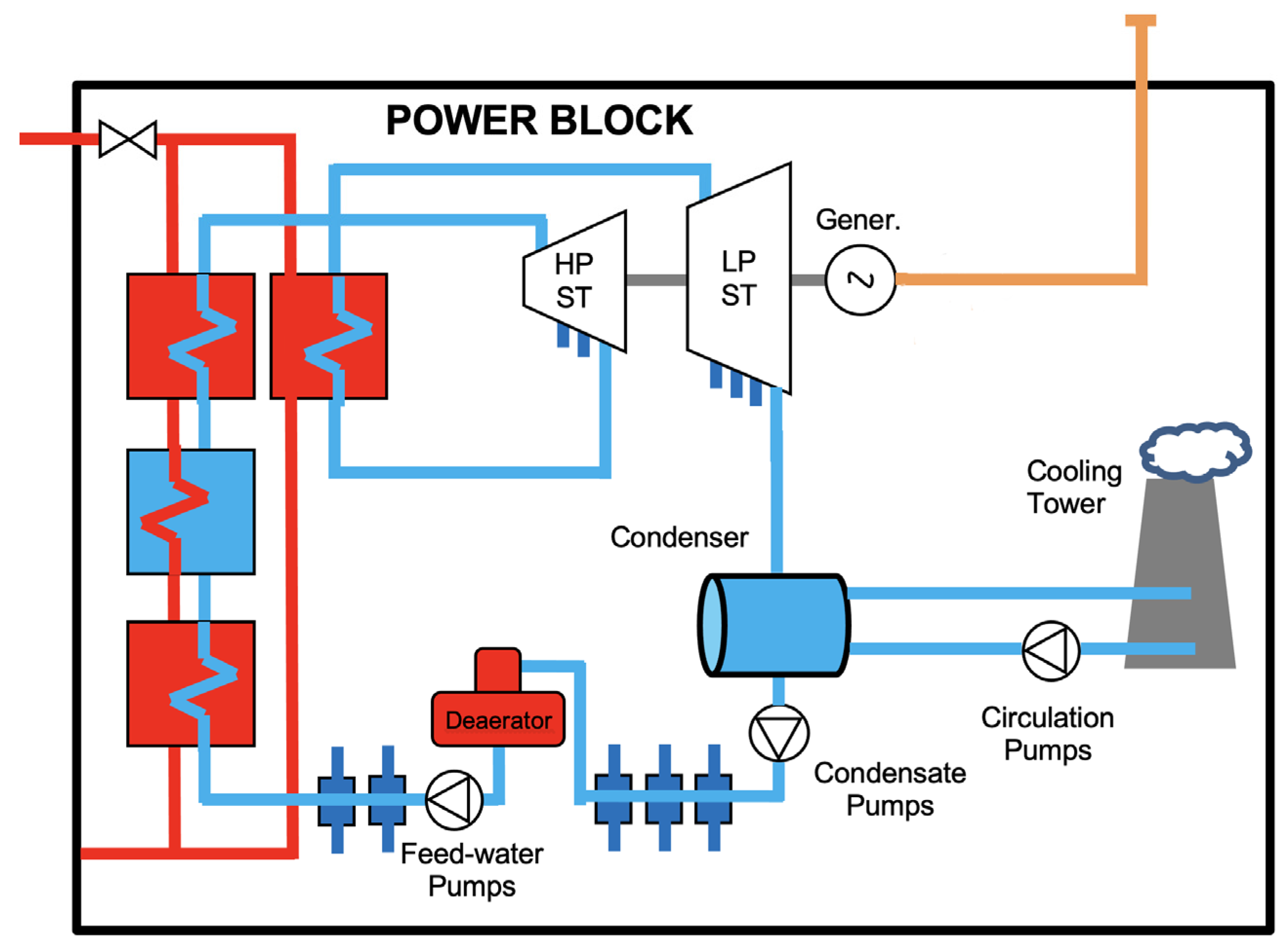
CSP has three main blocks: the solar field (SF), the thermal energy storage system (TES) and the power block (PB). The thermal energy absorbed by the solar field is transferred to steam at a high temperature. The Rankine cycle includes heaters, turbines, generators, condensers, and other elements. The PB of the CSP plant used as a reference in this paper is made of heat exchanger trains composed of reheaters, superheaters, boilers, and preheaters. This HX transforms the water into high-pressure, high-temperature steam, which enters the Rankine cycle. Also known as the water/steam cycle, it has both STs (steam turbines): a LPT (low pressure turbine) and an HPT (high pressure turbine). It has all the preheaters, one for each extraction. The steam is condensed in the ACC (air cooled condenser) or the cooling tower (selected according to localization and technical issues). The general layout of a CSP with TES is shown in Figure 1.
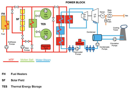
Figure 1.
Generic parabolic trough layout.
CSP technology is not yet widely deployed, with a global cumulative installation of only about 6 GW recorded in 2018. The CSP market reach $37.9 billion by 2019 [1]. The parabolic trough segment is expected to dominate the CSP market during the next decade. The CSP plants cumulative installation figures are remarkable, but the comparative with the enormous growth of PV installed capacity (more than 300 GWh and growing at increasing rates) shows that CSP’s development was much slower. PV generation has benefited from a huge reduction in installation costs, while cost reduction in CSP has been much lower. Thus, new improvements are required to allow CSP technologies to be able to compete in the energy pool with non-renewable energies and to expand to other countries like China, India, and MENA region ( Middle East and North Africa). The decrease in the levelized cost of energy (LCOE) at CSP plants cannot come exclusively from a reduction in the costs of the components because these have high costs due to the materials used and the difficulty of their manufacturing, but rather from improvements in their design and operation [2]. For this, it is not enough to design a plant that works, but rather have the right design for the meteorological, operating and retribution conditions of each site. In addition, as indicated in the study of the H2020 MUSTEC [3], the cost and performance of CSP plants depend not only on single components, but mostly on the know-how of how to assemble them and operate the entire station in the most efficient manner. Only a few companies have the knowledge needed to install and operate these plants. Improvements in decision-making regarding localization and plant design must be based on the most accurate performance model (PM). The CSP performance model (PM) is a model that simulates the amount of power and energy exported to the grid, among other operational variables. The more accurate the performance model, the better the plant design can be adjusted to the conditions of each project.
2. State of the Art: The CSP Power Block Performance Model
In the feasibility analysis of a CSP plant, electric production is estimated considering the site’s meteorological conditions and the schema of the solar field, the power block and the heat storage system. The behavior of the plant is simulated through the development of a CSP Performance Model (PM). The PM is used to estimate the LCOE (levelized cost of energy) [4,5] and to explore the tradeoffs between thermal storage capacity, cost, and other system parameters to optimize operation before the signature of the PPA (power purchase agreement).
CSP plant PMs began to be developed in the 1990s. SOLERGY [6] and EASY [7] were some of the first developments made at Sandia National Laboratories. The PM developed by Flagsol [8] has a very high level of detail. The one proposed by Patnode [9] simulates the solar field using TRNSYS software and uses simultaneous equation-solving software (EES) to model the Rankine cycle.
A very important model, due to its wide dissemination, is the system advisor model (SAM) [10]. SAM is a modeling open-source software for renewable energy systems, developed by the National Renewable Energy Laboratory (NREL). SAM combines annual time series power production models with financial models to estimate the levelized cost of energy (LCOE) and other metrics for renewable energy projects. At first, SAM used the general-purpose, commercial TRNSYS transient system-modeling software, but nowadays, the CSP models run in a new transient simulation framework written in C++, improving simulation time [11]. It is currently the standard software for CSP technologies because it is freely distributed and has adequate accuracy. This PM was developed to be used in the feasibility studies, and it did not aim to simulate transients. PMs can also be used in other stages of the project including O and M follow-up, and thus it is necessary to simulate all the operational conditions of the CSP plant. The Quasi-Dynamic Performance Model (QD-PM) [12], which was developed, among others, by some of the authors of this paper, is a PM that tries to offer the accuracy of dynamic models with less effort and by adapting to the different stages of the project life cycle. QD-PM has a modular approach, with a specific block for every system and with a finite-state machine that integrates the behavior of all of them. QD-PM introduces a quasi-dynamic approach to improve fitting in the transition between operation modes. QD-PM can be used either in the feasibility stage or in the design phase, as well as during plant performance follow-up. It has been used for many CSP plants, and it is still used nowadays. The main disadvantage is the amount of time needed to develop a specific model (about two man-months), which could be excessive for the very initial steps of the project.
Among all the blocks, the most difficult to be modeled is the power block. The PB uses a Rankine cycle, the same one as coal power. The only thing that changes is the heat source. The same software tools used for coal plant simulation can be used. For example, Llorente used Wolfram’s Mathematica 7 software as a development tool [13]. In the ITEA2 EUROXYSLIB European project, the ThermoSysPro library was developed to provide a generic library of the modeling and simulation of power plants. It was mainly designed for the static and dynamic modeling of power plants but can also be used for other energy systems such as industrial processes [14].
In QD-PM [12], the PB model is divided into a model of heat transfer and thermal inertia (implemented in Simulink) and a Rankine cycle model (implemented in Thermoflex software). All the exchangers have a static model, except for the boiler, which is simulated considering its thermal inertia and transient phenomena (as in the start-ups). To obtain a quasi-dynamic model, multiple static snapshots are made, with enough cases (the combination of the Thermoflex inputs) to model the Rankine cycle correctly. Although it is complex, it is quick compared to a complete dynamic model.
PB modeling is complex because it has many boundaries, which are defined by the supplier (warm-up curves, start-up curves, thermal shock, etc.). Its development implies a high computational cost. Speeding up PM development is a very relevant issue when a CSP project proposal is being prepared, allowing for shortening the time needed for each design test and allowing more possibilities to be evaluated.
3. Goal and Methodology
Reliable and accurate solar thermal power plant models already exist, but a decrease in the time required for their development would lower preparation costs and provide the necessary time margin to optimize proposals. Because the block that required the longest development time was the power block, the goal was to expedite its development using machine learning techniques.
The starting point of the research was the similarity between the PBs of different CSP plants. The designs of the solar fields and the thermal storage systems are highly dependent on the specific conditions of the location and the components used, but it is common for PBs to be very similar to each other. The underlying idea modeled performance with a black-box model, not the operation model, as was done in the physical PB. It was done using historical data from built plants. It was desired that the modeling should reflect all operating situations and be as simple as possible.
The model’s scope was to accurately predict the gross power generated by the PB in every moment. To do so, from a thermal process point of view, several variables were involved:
- HTF mass flow passing through the PB.
- HTF temperature at the inlet of the PB.
- Ambient temperature.
- Relative humidity.
These inputs defined the amount of thermal power entering the steam turbines (ST) and the vacuum in the ACC or condenser. Nevertheless, other variables could be considered. The Figure 2 shows the boundaries of the model, what was considered and what could be expected.
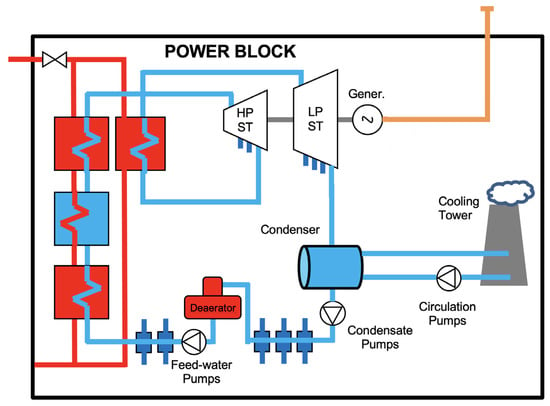
Figure 2.
PB diagram.
To develop the model, the machine learning technique must be robust regarding the appearance of outliers and with a great capacity for generalization (avoiding overtraining issues) For this reason, it was decided to use support vector regression (SVR) and no other options such as artificial neural networks.
4. Support Vector Regression
Supervised learning represents an alternative to physical modeling. It is based on a representative data set wherein the values of the input and output variables are known, and the relationship between the dependent variables is determined as a function of the independent or input variables. The modeling problem contemplated here required a quantitative answer, and it was, therefore, considered a regression problem.
Within supervised learning, there are a wide variety of techniques such as Bayesian statistics, decision trees, genetic programming and neural networks, to name a few of the most used. More recently, support vector machines (SVM) and specifically, support vector regression techniques (SVR), have shown their usefulness. In [15], different modeling techniques were compared against the electricity production of hydropower plants, using SVM as the technique, with more accurate results. Their objective was to define the relationship between the input and output variables as a geometric optimization problem, described as a convex quadratic optimization problem with linear constraints, which could be solved by non-linear optimization.
Support vector machines were defined in the work on statistical learning theory by Vapnik in the 1990s [16]. They were raised to solve binary classification problems, but they were adapted to solve classification and regression problems. It is intended to select a separation hyperplane equidistant to the closest examples of each class. For this, only the data with a distance from the hyperplane greater than the “distance margin” are considered (support vectors). This technique can be used for modeling problems such as regression (SVR, support vector regression). A good description of the basis of SVR can be found in [17].
This operation, as a binary classifier, can be used to solve multidimensional function estimation problems. For this purpose, the regression hyperplane best-suited to the training dataset was selected. A margin distance was considered that expected all the data to be in an n-dimensional band or tube around the described hyperplane, thus ensuring that they were less distant than the margin distance. To define the hyperplane, the support vectors were used, which were the farthest points from the hyperplane margin.
In a case with two inputs and for a dataset of training data
(x1, y1), (x2, y2), …, (xi, yi), ⊂ X i = 1, 2, …, n.
Given a linear function as
where W is the weight vector, b the bias term, SVR searches for the function where the deviation from the training dataset point is less than ε, with minimum W. This search is transformed into a non-linear optimization problem that can be solved in its dual form using the Lagrange method.
SVR is a technique that tries to optimize the generalization bounds. They rely on defining a loss function that ignores errors situated within a certain distance from the true value. This type of function is often called an epsilon-intensive loss function. The input data is mapped on an n-dimensional feature space, using a nonlinear mapping function, and a linear model is constructed in this feature space.
SVR accuracy depends, extremely, on the selection of some parameters: the distance margin, the punishing coefficient (parameter C) that determines the punishment for experiential error (greater values implies more overtraining risks but smaller fitting) ) and the hyper-parameters of the kernel function
5. Data Treatment
Machine learning requires a data set with all the information needed for generalization. As heat flow depends on solar field output, a whole year’s data is considered representative of a CSP plant’s performance.
The training and validation of the SVR model followed these steps:
- SVR Training: A whole year of data were used to train the model and tune the parameters. The data were obtained from a plant situated in Spain that was denominated as Plant A, with a rated power of 50 MWe;
- Validation with new data from the same CSP plant A. A new complete year of data was collected after the year used for training, and it was used to validate the model’s performance.
- Validation of this modeling methodology for other CSP plants of any power. Steps 1 and 2 were done using data from another plant, denominated here as Plant B. This plant was in North Africa and had a rated power of 120 MWe.
All the data used were captured from the data acquisition systems of plants under normal operation. The variables downloaded from the data acquisition system of each plant data log were:
- DNI (direct normal irradiation) from all the meteorological stations.
- Ambient temperature from all the meteorological stations.
- RH (relative humidity) from all the meteorological stations.
- Flow through the SGS (steam generation system).
- SGS inlet temperature.
- Date.
The data corresponding to two years of operation of Plant A and one year of operation of Plant B were collected. All data was averaged considering 1 min intervals, obtaining a set of 1,051,200 records from Plant A’s data logger and 575,600 records from Plant B’s logger. Previous works [12] determinate that a timestep of 3-5 minutes is enough to see the effect of fast transients due to quick weather changes. Plant A’s dataset was divided into two, with each corresponding to a complete natural year, from January 1st to December 31st. The first year was used for training and the second one for validation purposes. In Plant B, the same procedure was applied. with datasets of six months each.
The data quality was very good. In the previous data treatment, data related to the following situations were deleted:
- Outliers or incorrect values, mainly from problems in data acquisition (sensor offset in the flow meter, error in the communication of the signal in meteorological stations).
- Null values.
- Data from the time intervals when due to different circumstances, the plant was not in operation (breakdowns, maintenance, operation tests).
The number of outliers was so low (far less than 1% of the total data) that deleting them was considered the best choice, discarding other alternatives. It was detected that the flow meter measurement was higher than zero when the plant was stopped. Thus, a threshold was established to assure this flow meter offset was not considered.
6. Model Development
The decision about the selection of the input variables was based on extensive experience in CSP non-data-driven modeling and the controls of several plants already in commercial operation. The starting point was to consider that the system would be able to follow the transients without information coming either from the solar field or from the thermal energy storage. However, the solar field had relevant thermal inertia, and there were some concerns about the necessity of introducing other inputs as irradiation values (with some delay reference to the thermal inertia) and the state of the heat storage.
Relative humidity and the ambient temperature are inputs in the usual Rankine physical model. Nevertheless, the instrument reliability and tolerance of the hygrometer were the reasons for not including humidity as one of the input variables. The inputs which data was collected are the hot temperature fluid (HTF) flow and temperature, measured at the inlet of the PB. The gross power was selected as the output variable.
The training and fitting of the model was conducted using the Statistics and Machine Learning Toolbox of MATLAB R2020b, of MathWorks, Inc. (USA). This is a widely used numeric computing environment. The toolbox included the functions needed to train and fit the model. In addition, the SVR model could be exported easily to Simulink, allowing its integration with PMs like QD-PM [12].
The generalization and robustness of SVRs are their key advantages, and they are based in the ability to solve nonlinear problems using kernel methods. The main inconvenience is the computational cost, which grows more than linearly with the increase in number of records. Using the newest, 8-core Intel i7 CPU allowed training the model in minutes. However, one of the aspects that greatly hinders the training phase of an SVR is the definition of the kernel used to increase the dimensions of the data set. Although there are some guidelines, it is necessary to try several options and then carry out a model adjustment. Given the number of records involved as well as the evaluation of the kernels and their hyper-parameters, the computational cost of all the training is huge.
A screening was done to try to establish the best kernel function for the system and the inputs required for proper accuracy. The kernels used were lineal, polynomial and Gaussian. Training was achieved using the kernel function available in the Statistics and Machine Learning Toolbox of MATLAB, which defined the function, as can be seen in Table 1.

Table 1.
Kernel functions.
With the training set of Plant A, the results with the linear kernel were quite bad, but the Gaussian kernel and the polynomial offered very good models with adequate hyper-parameters. For all kernels, it was necessary tunning the parameters using a grid search. To evaluate accuracy, 15% of the data were removed from the training test and used to evaluate the performance of the model. The model estimation fit the output data very accurately, and the best results were obtained using the polynomial kernel, by a slight difference.
To check if ambient temperature was a relevant input due to its relatively small variation during the periods of operation of the plant, some models were trained while removing it from the input set. The comparison was made using a new, complete year of data, and the results are shown in the next section.
7. Validation, Plant A
This model was developed to be included in a CSP plant performance model, in the same manner as the QD-PM. To ensure the generalizability of the model, the SVR models obtained after training faced an entirely new data set, corresponding to a full year of operation. The aim was not only to verify overall accuracy, but also to ensure that the model showed the evolution in the transients. As transients corresponded to relatively small periods of time, the model might not have had precision in these areas, but it showed a small average fit error.
The best SVR models (kernel and hyper-parameters) were selected in the training stage, according to the accuracy of the estimation of the 15% of the data previously removed from the data test. This SVR models were used to simulate the complete year, using data from the year following the one used in training. We included in the comparison SVR models that included, or not, ambient temperature as inputs, according to the naming showed in Table 2. OPT-1 and OPT-2 were the most accurate models using Gaussian kernels, both not including and including ambient temperature as inputs. The OPT-3 and OPT-4 were the models developed using polynomial kernels. The OPT-5, which used a linear kernel, was included to allow comparison.

Table 2.
Validation with Plant A data. (Tamb is the ambient temperature, Tin is the PB inlet temperature and Fin is the PB inlet flow).
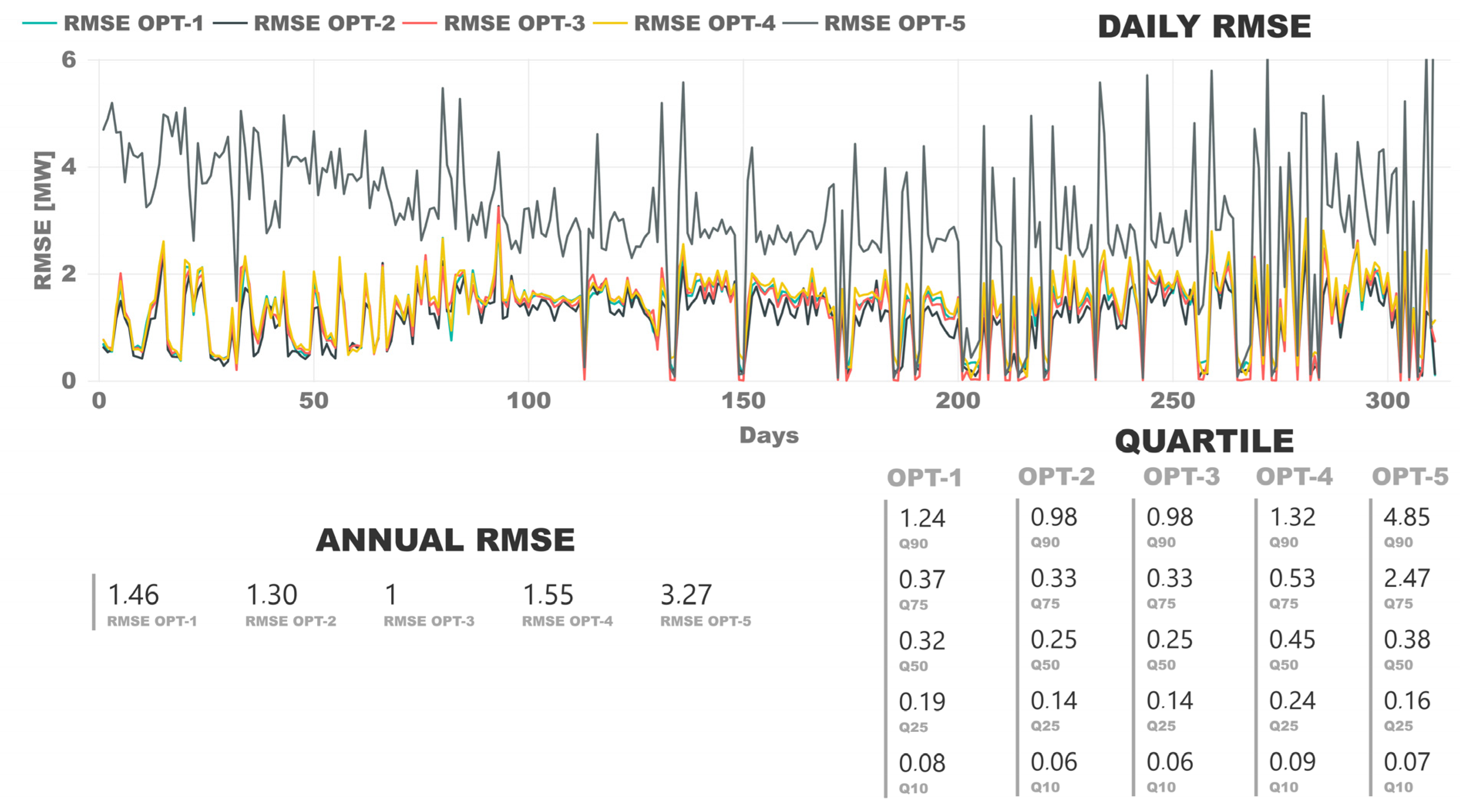
The validation of the trained models was the process wherein the models’ outputs were compared with real observations to judge correspondence with reality. The validation process used, as input, a complete year of data that was not used in the training phase. As a first step, data were grouped on a daily and yearly basis. The root mean square error (RMSE) was calculated for each period. In Figure 3, the graph shows the values of the RMSE of each day (from 1 January, day 1 in the graph); on the left lower canvas, the RMSE is shown for the complete year period; and on the right, the quartiles of the RMSE of cumulative daily for each SVR model.

Figure 3.
Comparison of model RMSE with validation data.
The linear kernel had the worst results, as expected according to the training stage. The Gaussian and polynomial kernels had good accuracy. The best fit was obtained with the OPT-3 (polynomial kernel, including ambient temperature). The days when the daily RMSE was zero usually corresponded to situations in which the plant had been shut down for most of the day. It should be remembered that the plant had a rated power of 50 MWe, and that the instantaneous power values varied between 20–30 and 55 MWe, as the plant could operate 10% above nominal. The gross power as output was simulated every minute. The RMSE values below 1 MW, in 90% of the cases, and always with some exceptions below 2 MW, were of extraordinary accuracy, exceeding the authors’ previous expectations, taking into account that this data came from a real CSP plant in commercial operation and subjected to various meteorological conditions and operating modes.
The OPT-1 and OPT-4 models were trained without using ambient temperature as an input. The results of both models were good, but worse than those in which ambient temperature was included as input. This occurred independently of the kernel. Therefore, it was considered that although the ambient temperature data had a small variance, it was sufficiently significant, and its introduction allowed for a better fitting model. On the other hand, if such data were not available for an installation, this would not prevent the use of these data to generate the model of its PB, since the results obtained would be sufficiently good and representative.
However, to be accurate regarding average values was not the only goal of model development. It was also important that the model could follow different operation modes. Under normal operation mode, every day, the plant started up when irradiation was enough, rose to nominal operative mode, gave heat to the TES if it was possible, used the heat flow from the TES to extend operation when irradiation decreased and so on, day by day. There were many different operation issues over all the seasons, and the model needed to reflect that. This was not as relevant in terms of average values because most of the gross power was produced in nominal operation, but it was essential for the model to be used in O and M supervision.
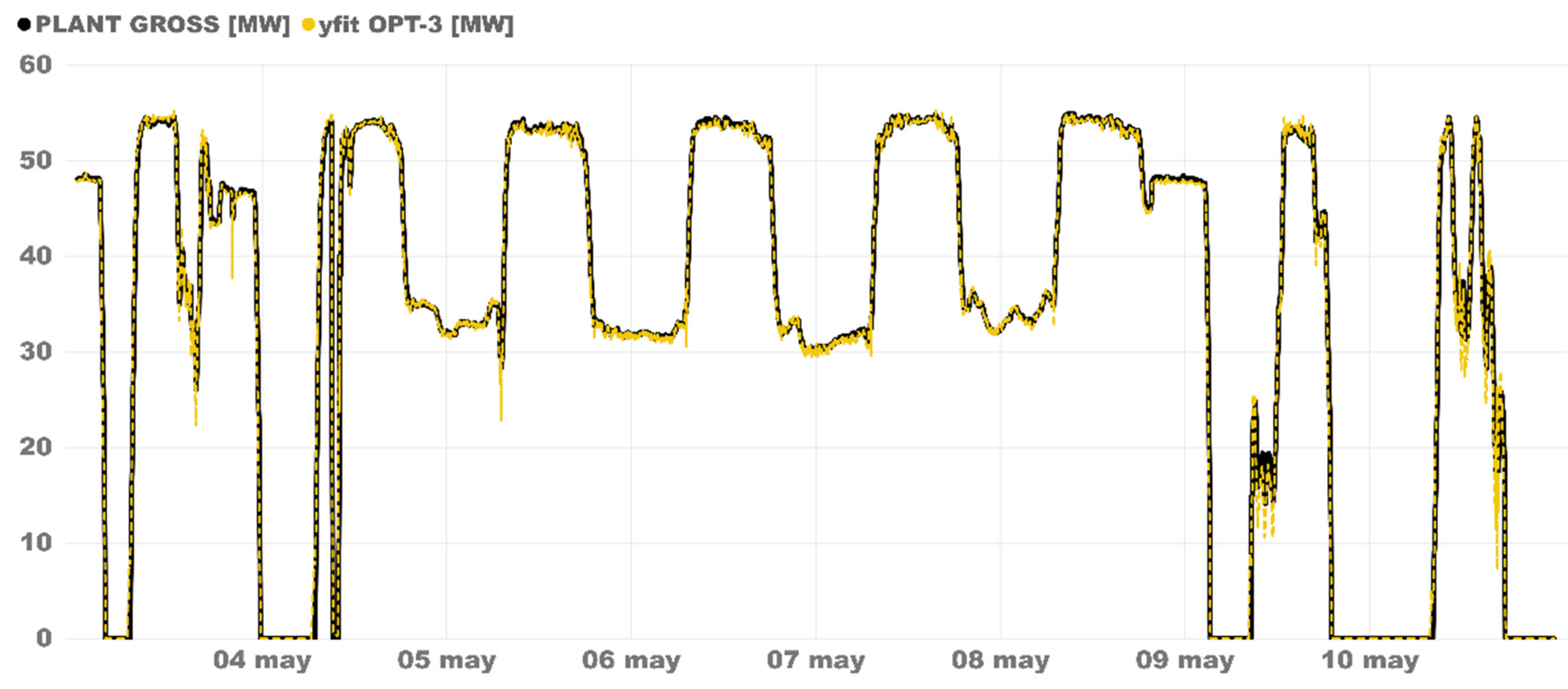
We studied how the model followed transients, with extremely satisfactory results. The fit was extremely good in all conditions, including the unusual ones. In Figure 4, the best SVR model (OPT-3 polynomial kernel) outputs are showed against validation data in a week where the operation was very unusual. From May 5th to 9th, Plant A was on 24 h continuous production. This only happens when there is enough DNI to produce and charge at a nominal rate for many hours. In this case, the discharge rate was diminished by a little to maintain the production untilthe next sunrise using the heat storage output. This operation mode was very interesting because it would entail a lower O and M cost. In addition, May 4th and the weekend were very unusual. As can be seen in Figure 4, the SVR model fits extraordinarily well with the real data. The model overreacts a little in the transients and predicts a higher reduction when the plant reduces the load drastically, but the effect of this inertia disappears within a very few minutes. At the end, the desired goal of modeling physical behavior rather than the combination of the operation mode and the equipment was achieved.
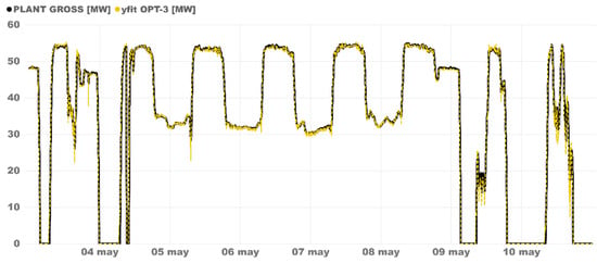
Figure 4.
OPT-3 model validation in a continuous operation week.
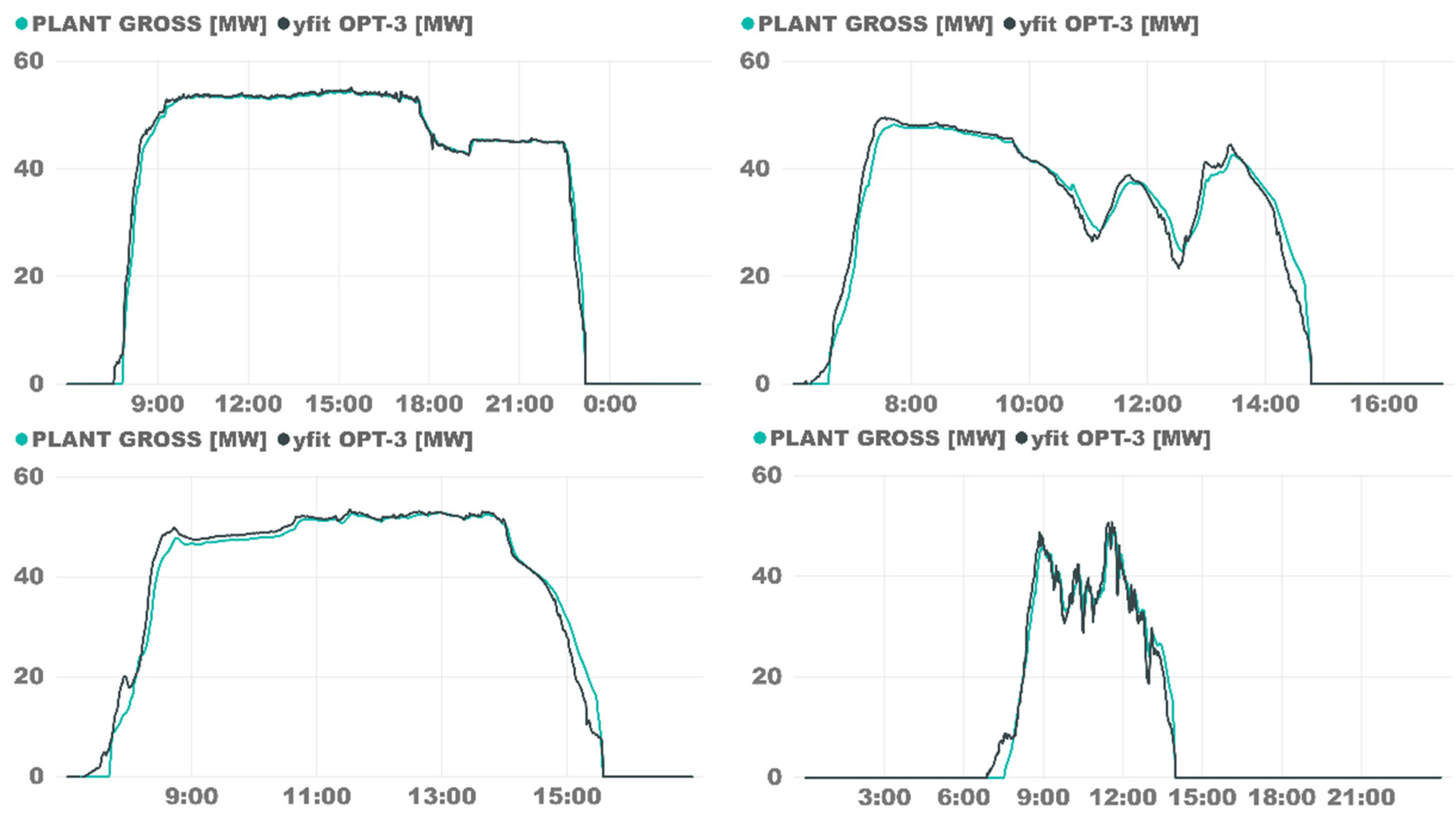
Figure 5 shows several days in detail; from now on, in the daily plots, the black line is the gross power predicted, and the turquoise blue is the measured plant gross power. The upper left graph was an almost-standard day, with nothing special to highlight aside from the transient before the TES discharge, which was not properly done. In the contiguous plot, the day was far worse and much unstable than the first one; the SVR model keeps its accuracy, but it can be observed that the fit curve always has a delay compared to the real gross power. The first graph in the second row was a day in which the TES was barely used for charging and discharging; the steady state was predicted almost perfectly, but the transient had a higher error. Transient effects have greater variability and complexity and depends on the previous stationary conditions, but the simulation fits with very low error.. The last graphs (down, right) refer to a cloudy day, which is the most complicated situation to predict. Nevertheless, the model was capable of accurately predicting the output.
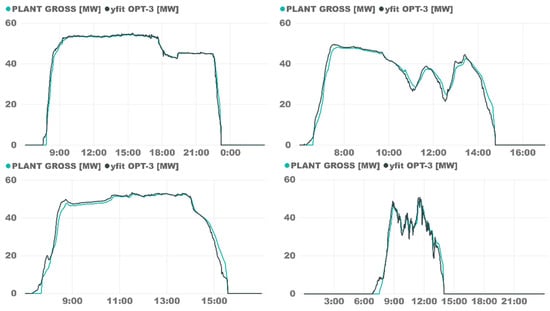
Figure 5.
OPT-3 model validation on specific days.
It can be noted that all days displayed in Figure 5 have one point in common: The model is not fully capable of having the same accuracy at the start-up as it has at the shutdown. The start-up process was much more complex, depending on several constraints that were handled differently by one operator or another.
8. Validation in Another Plant: Plant B
The desired goal was to be able to simulate any PB from historical data for any plant, not just for one specific plant. This would permit to generating a PB model library that could be used in the design of new CSP plants. The Plant A, used in the previous part as source of the data, was in operation from some years. Their operators are very experienced, and the operative is quite stable. To evaluate if this way to develop the PB model is applicable in any case, a very different CSP plant was selected: Plant B. The first difference is the nominal power of the Plant B double the Plant A one. The second difference is Plant B is more recent, and it is necessary to use the data from the starting of their operation, when the operator is beginning the learning curve. Due it had only been in operation recently, only one year’s data was available. The training and validation were done in the same way as with the Plant A data. As the polynomial kernel offered the best results, we used it in reference training models with and without ambient temperature (OPT-7 and OPT-8 models). We also trained comparative reference models with Gaussian (OPT-6) and linear (OPT-9) kernels. In Table 3, a list of the models used in the validation is shown.

Table 3.
Validation with Plant B data. Tamb is the ambient temperature, Tin is PB inlet temperature and Fin is the PB inlet flow.
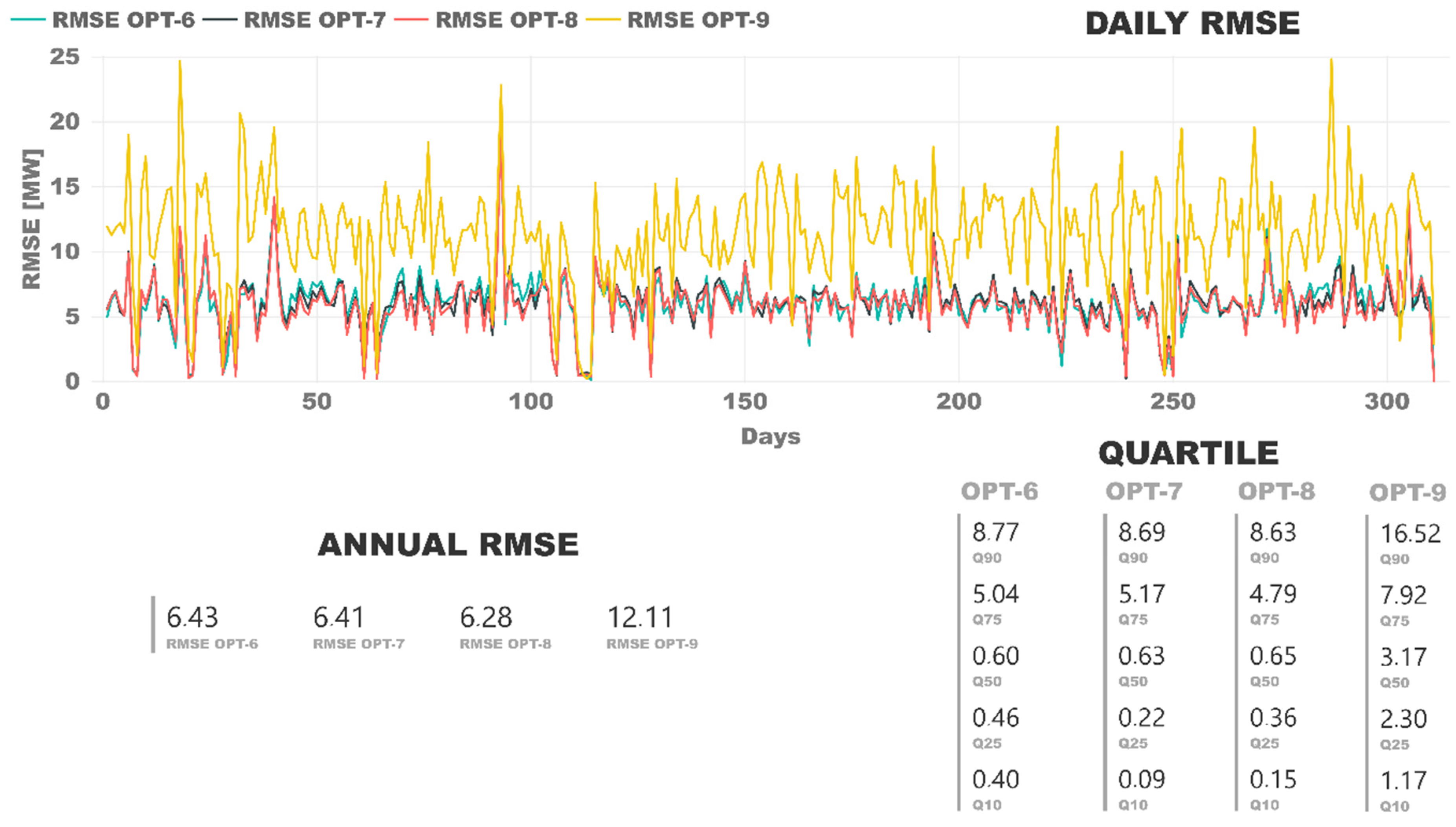
Figure 6 shows the summary of the RMSE values, on average, for a day and for a complete year. It should be noted that Plant B had much higher-rated power, which explained why the RMSE values were greater than in Plant A. The annual analysis established that the worst model was OPT-9, which was a linear kernel-based SVR model, as in Plant A. Both the Gaussian and polynomial kernels were again the most accurate ones, and the polynomial kernel was the best option. The best SVR model was the OPT-8, trained using a polynomial kernel, as in Plant A. However, the results compared to the Gaussian kernel were so close that both kernels were good choices to train the SVR model.
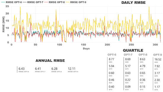
Figure 6.
Comparison of Model RMSE with Plant B validation data.
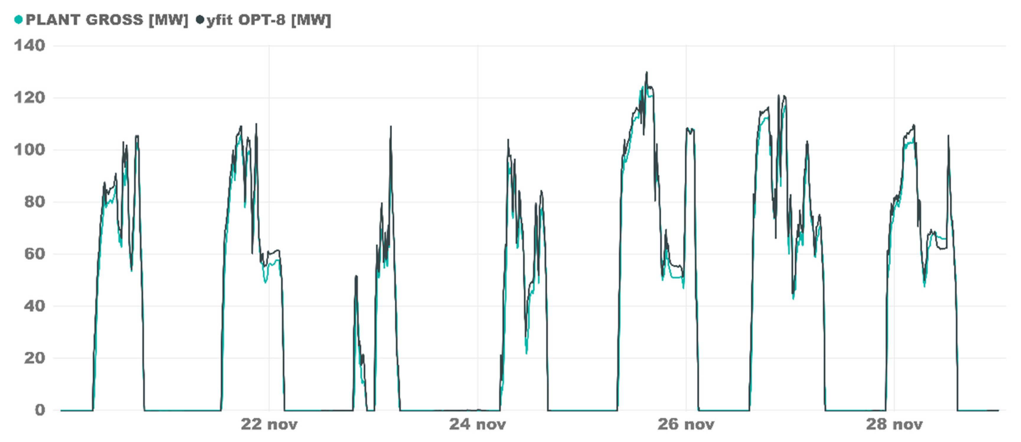
An overview of how the model predicted the gross power generation is shown in Figure 7. On the graph, several complex transients are shown such as the big transients between SF-only mode and discharge-only mode. Not only the stationary operation is simulated, also, the ramp-up and shutdown operations was predicted almost perfectly.
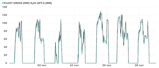
Figure 7.
OPT-8 Plant B model validation in a continuous operation week.
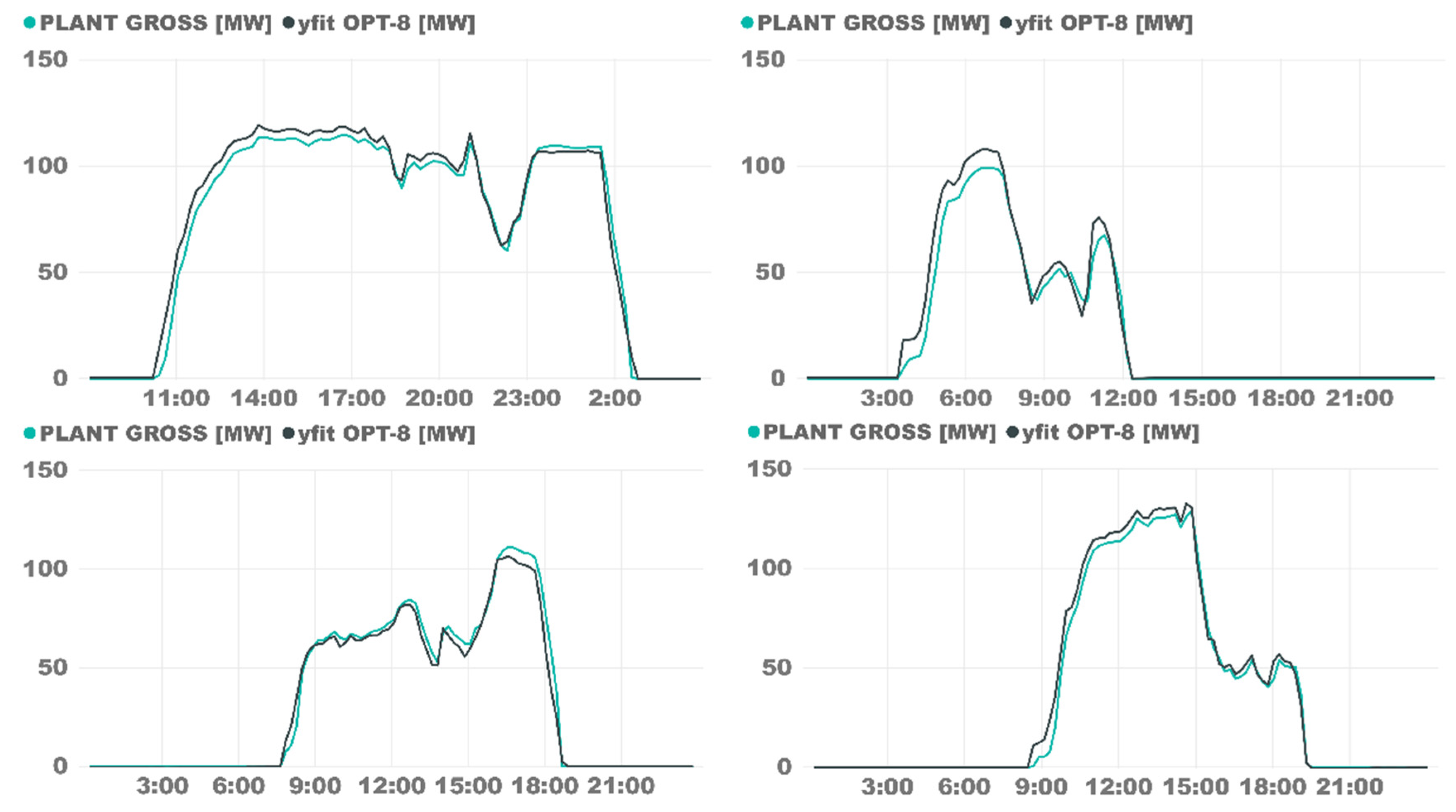
The dataset of Plant B had a lower quality due to the state of the plant (raising the operation management learning curve) and the much more complex data format. Despite this, the SVR model was accurate in all operation models, as in Plant A. Figure 8 shows how the model fits real outputs as a stratified sample of the different operational situations. In the upper left graph, there is a sunny day with a big transit between SF-only mode and TES discharge operation, in which the model fits real outputs with high accuracy. The contiguous plot is of a cloudy day with higher operational difficulty; however, the SVR model also predicted correctly, with some overestimating. The plots in the lower row represent not-so-usual situations; the left one is a prioritizing storage situation, and on the right, there is a situation involving discharging the TES at a lower load. Even so, the SVR model was capable of accurately predicting the outcome.
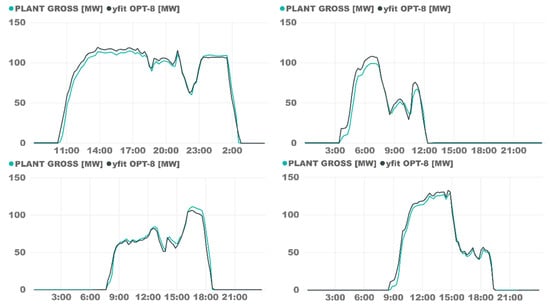
Figure 8.
OPT-8 plant B model validation on specific days.
9. Conclusions
Optimizing the design and the operation of CSP plants is necessary to increase their competitiveness against other renewable energy sources. For bids’ presentation stages, initially, and for the phases that follow, it is necessary to have a performance model as accurate as possible.
This model incorporated blocks that represented all the main systems of the plant. The block that required by far the most effort and cost in its modeling was the PB. Because these systems can be similar in some plants, historical data could be used for modeling. PB modeling requirements include: accuracy, an assurance of generalization, and the ability for reproducing transients. The techniques based on SVM, such as SVR, introduced characteristics that made it possible to ensure generalization, which was why they were the ones chosen for this development. A full year of data taken at one-minute intervals was used for model training. After the tests, very good results were obtained with a polynomial kernel. The SVR models were validated using a new complete year of data, corresponding to a later period. The fitting was excellent in the most common situations. It recognized the transients but overestimated certain variations (not considering all the thermal inertia of the system). To ensure that this method was generally applicable, the process was repeated, using data from another plant of a very different size. The validation showed the same excellent fitting. Therefore, SVR was a suitable tool to simulate this system. It offered results that allowed for composing models that could be used as PM blocks of new designs that used the same PB, allowing creation from a library of PB models.
The main advantages were:
- The accuracy of the model was extremely good in all situations, including transients.
- Development efforts were reduced. The human effort of the development of a physical model could be a Man-Month (or more). If we have data from other plants with similar PBs, we can develop an SVR in a week and a half.
As PBs are quite similar in many CSP plants, if their data are available, it is possible to quickly develop a SVR model of the PB and integrate it into a complete CSP performance model, offering very good accuracy with a very reasonable development time. As CSP project revenues are dependent on the relationship between the initial investment and the net energy produced in the life cycle, having a better CSP performance model allows for the reduction of the financial risk of the project.
Author Contributions
Problem definition and conceptualization: R.P.M.; Methodology: J.V.A.C., M.A.V.B.; Model training: A.G.G.; Validation: A.G.G., J.V.A.C. and A.R.F.; Writing: A.G.G., J.V.A.C. All authors have read and agreed to the published version of the manuscript.
Funding
This research was funded by the GRUPIN program of the University of Oviedo.
Institutional Review Board Statement
Not applicable.
Informed Consent Statement
Not applicable.
Conflicts of Interest
The authors declare no conflict of interest.
Glossary
| ACC | Air cooled condenser |
| CSP | Concentrated solar power |
| DNI | Direct normal irradiation |
| HPT | High pressure turbine |
| HTF | Heat transfer fluid |
| HX | Heat exchangers |
| LCOE | Levelized cost of energy |
| LPT | Low pressure turbine |
| O &M | Operation and maintenance |
| PB | Power block |
| PM | Performance model |
| PPA | Power purchase agreement |
| SAM | System advisory model |
| SF | Solar field |
| TES | Thermal energy storage |
References
- Vision Gain. Solar Tracker Market Report 2019-2029; Vision Gain: London, UK, 2019. [Google Scholar]
- Siva Reddy, V.; Kaushik, S.C.; Ranjan, K.R.; Tyagi, S.K. State-of-the-art of solar thermal power plants—A review. Renew. Sustain. Energy Rev. 2013, 27, 258–273. [Google Scholar] [CrossRef]
- Lilliestam, J. Whither CSP? Taking stock of a decade of concentrating solar power expansion and development, deliverable 4.2 of the H2020 project. MUSTEC 2020, 57. [Google Scholar]
- Bishoyi, D.; Sudhakar, K. Modeling and performance simulation of 100 MW LFR based solar thermal power plant in Udaipur India. Resour. Technol. 2017, 3, 365–377. [Google Scholar] [CrossRef]
- Zhang, Y.; Smith, S.J.; Kyle, P.; Stackhouse, P.W. Modeling the potential for thermal concentrating solar power technologies. Energy Policy 2010, 38, 7884–7897. [Google Scholar] [CrossRef]
- Stoddard, M.; Faas, S.; Chiang, C.; Dirks, J. SOLERGY- A Computer Code for Calculating the Annual Energy from Central Receiver Power Plants; Sandia National Laboratory: Albuquerque, NM, USA, 1987. [Google Scholar]
- Lippke, F. Simulation of the Part-Load Behavior of a 30 MWe SEGS Plant; No. SAND-95-1293; Sandia National Lab.: Albuquerque, NM, USA, 1995. [Google Scholar]
- Price, H.W. Validation of the FLAGSOL Parabolic Trough Solar Power Plant Performance Model; No. NREL/TP-471-7297; CONF-950336-19; National Renewable Energy Lab.: Golden, CO, USA, 1994. [Google Scholar]
- Patnode, A. Simulation and Performance Evaluation of Parabolic Trough Solar Power Plants; University of Wisconsin-Madison: Madison, WI, USA, 2006. [Google Scholar]
- Wagner, M.; Blair, N.; Dobos, A.A. Detailed Physical Trough model for NREL’s Solar Advisor Model: Preprint: 11; No. NREL/CP-5500-49368; National Renewable Energy Lab.: Golden, CO, USA, 2010. [Google Scholar]
- Dobos, A.; Neises, T.; Wagner, M. Advances in CSP Simulation Technology in the System Advisor Model. Energy Procedia. 2014, 49, 2482–2489. [Google Scholar] [CrossRef]
- Gonzalez, A.G.; Cabal, J.V.A.; Montequin, V.R.; Balsera, J.V.; Menéndez, R.P. CSP Quasi-Dynamic Performance Model Development for All Project Life Cycle Stages and Considering Operation Modes. Validation Using One Year Data. Energies 2020, 14, 14. [Google Scholar] [CrossRef]
- Llorente García, I.; Álvarez, J.L.; Blanco, D. Performance model for parabolic trough solar thermal power plants with thermal storage: Comparison to operating plant data. Sol. Energy. Oct. De 2011, 85, 2443–2460. [Google Scholar] [CrossRef]
- Hefni, B.E. Dynamic Modeling of Concentrated Solar Power Plants with the ThermoSysPro Library (Parabolic Trough Collectors, Fresnel Reflector and Solar-Hybrid). Energy Procedia. 2014, 49, 1127–1137. [Google Scholar] [CrossRef]
- Operacz, A.; Szeląg, B.; Grahl-Madsen, M. Possibility of the Modelling of Electricity Production from Hydropower0; Jóźwiakowski, K., Kasprzyk, M., Eds.; EDP Sciences: Ulis, France, 2019; Volume 86, p. 00008. [Google Scholar]
- Cortes, C.; Vapnik, V. Support-vector networks. Mach Learn. Septiembre De 1995, 20, 273–297. [Google Scholar] [CrossRef]
- Smola, A.J.; Schölkopf, B. A tutorial on support vector regression. Stat. Comput. 2004, 14, 199–222. [Google Scholar] [CrossRef]
Publisher’s Note: MDPI stays neutral with regard to jurisdictional claims in published maps and institutional affiliations. |
© 2021 by the authors. Licensee MDPI, Basel, Switzerland. This article is an open access article distributed under the terms and conditions of the Creative Commons Attribution (CC BY) license (https://creativecommons.org/licenses/by/4.0/).


