Abstract
Reservoir modeling to predict shale reservoir productivity is considerably uncertain and time consuming. Since we need to simulate the physical phenomenon of multi-stage hydraulic fracturing. To overcome these limitations, this paper presents an alternative proxy model based on data-driven deep learning model. Furthermore, this study not only proposes the development process of a proxy model, but also verifies using field data for 1239 horizontal wells from the Montney shale formation in Alberta, Canada. A deep neural network (DNN) based on multi-layer perceptron was applied to predict the cumulative gas production as the dependent variable. The independent variable is largely divided into four types: well information, completion and hydraulic fracturing and production data. It was found that the prediction performance was better when using a principal component with a cumulative contribution of 85% using principal component analysis that extracts important information from multivariate data, and when predicting with a DNN model using 6 variables calculated through variable importance analysis. Hence, to develop a reliable deep learning model, sensitivity analysis of hyperparameters was performed to determine one-hot encoding, dropout, activation function, learning rate, hidden layer number and neuron number. As a result, the best prediction of the mean absolute percentage error of the cumulative gas production improved to at least 0.2% and up to 9.1%. The novel approach of this study can also be applied to other shale formations. Furthermore, a useful guide for economic analysis and future development plans of nearby reservoirs.
1. Introduction
In recent decades, unconventional oil and gas resource development has been carried out, mainly in the United States and Canada. This has been facilitated by the development of horizontal drilling and multi-stage hydraulic fracturing technology. Since unconventional reservoirs have nano-Darcy permeability, horizontal drilling with multi-stage hydraulic fracturing is used to expand the hydrocarbon drainage to maximize production [1]. Reservoir modeling for productivity prediction in such systems is an extremely complicated task, owing to the need to simulate fluid flow in a network of induced natural fractures coupled to geomechanical effects and other processes such as non-Darcy flow, adsorption-desorption and water blocking [2,3,4]. Various numerical simulation methods that simulate multi-stage hydraulic fracturing behavior in horizontal wells are continuously being studied [5,6,7,8,9].
However, reservoir simulation models considering complex geological factors cannot realistically be applied to this technique as the computational load quickly becomes large and time-consuming. Applying technologies such as massively parallel execution can accelerate the execution of large-scale reservoir simulation models. However, complex flow phenomena of unconventional reservoirs combined with poor field data make the results of any reserves estimation highly uncertain.
Thus, the decline curve analysis (DCA) proposed by Arps [10] is still widely used to predict the reserves of conventional and unconventional wells. The DCA to be applicable, a reservoir should be in boundary dominant flow (BDF) with constant bottom hole pressure. However, due to the low permeability of the shale formation, the linear flow in the early stage of production is dominant. To overcome this limitation, various new DCA methods have been proposed. It is divided into multi-segment Arps based DCA [11,12,13] and post-Arps single-segment DCA method [14,15,16,17].
DCA requires a wise judgement based on an engineer’s experience or insight. In the case of Arps equation, it is necessary to select decline exponent (b) and decline rate (D), According to Power Law Exponential Decline (PLED), Duong and Stretched Exponential Production Decline (SEPD) method and the Logistic Growth Model (LGM), depending on the flow domain regime or the amount of production data, the engineer’s prediction results can lead to positive or conservative predictions. Hu et al. [18] compared the suitability of Arps and post-Arps single-segment DCA methods from Eagle Ford shale wells. As a result, the multi-segment DCA method was most suitable. Duong model overestimated, and SEPD underestimated the estimated ultimate recovery (EUR), so both methods found a similar problem of finding the point of switching from linear flow to BDF flow. A series of DCA method is greatly useful for predicting future production profile with little data. However, it is difficult to predict pre-drilling productivity or reflect the influence of factors related to hydraulic fracturing and well completion of shale formations.
Thus, in recent years, researchers have begun to develop alternative models to replace reservoir simulation and DCA model [19,20,21,22]. For example, some studies have proposed an advanced, fast analytical model based on complex analysis methods [23,24]. It is an analytical model but requires only a minimum of input parameters and can be achieved with a simple spreadsheet. Furthermore, a probabilistic methodology has been developed to evaluate the economics of a shale gas project while taking into account the uncertainty of the input parameters [25]. For production prediction, a proxy model or a surrogate model can be developed to approximate the solution of a complex storage simulation model. It is not possible to produce exactly the same output as the reservoir model using a much less complex proxy model. However, it can be quite beneficial to roughly calculate the desired output. The proxy models developed in petroleum engineering can generally be classified into four groups according to the development approach: statistics-based approaches, reduced physics approaches, reduced-order modeling approaches and machine learning and artificial intelligence (AI)-based technologies.
In recent years, many studies have applied data-driven machine learning techniques to analyze the hydrocarbon production of shale reservoirs. Mohaghegh [26] quantitatively assessed the impact of shale gas development by analyzing the correlation and pattern recognition between productivity and other factors such as rock mechanical properties, hydraulic fracturing data and reservoir properties. Exploratory data analysis (EDA) has been used to predict the cumulative production of a shale play using a variety of supervised learning techniques, such as regression analysis, support vector machines (SVM) and gradient boosting tree machines (GBM) [27]. In addition, a classification and regression tree (CART) has been performed using regression analysis to identify the importance of input data and to select useful input data for production prediction, to improve the predictive performance of the model [27,28,29,30,31].
Alabbodi et al. [32], Mohaghegh et al. [33] and Li et al. [34] developed a data-driven artificial neural network (ANN) model to predict the EUR of shale reservoirs. In addition, Han and Kwon [35] and Han et al. [27] conducted a study to improve the predictive performance of the model using cluster analysis, an unsupervised learning technique, using a machine learning model and data from Eagle Ford shale reservoirs. In recent studies, a variety of data mining approaches have been performed for the hydraulic fracturing design for reservoir in the Montney formation and the completion of well data. In addition, various supervised learning models were applied to predict productivity [36,37,38,39]. A novel approach using principal component analysis (PCA) was proposed to predict the production behavior of the shale reservoir. PCA creates new low-dimensional components that can better describe the data distribution of multivariate data. The main variables that simulate the early-mid-term behavior of the shale reservoir were extracted [40,41].
The above studies are infancy production prediction studies using data mining techniques. In addition, it has a limitation in that it is a model that does not reflect categorical variables related to well information as a result of hydraulic fracturing and well completion. The main purpose of this study is to elucidate the methodology when using a data-driven deep learning proxy model utilizing a large amount of database from shale reservoirs. We propose a procedure to apply sensitivity analysis of hyperparameters in deep learning, machine learning based variable importance analysis (VIA), and PCA to build reliable and accurate predictive models.
This paper consists of the following. First, we present an overall data preprocessing process that involves identifying characteristics and types of data based on statistical analysis, as well as identifying outliers inherent in datasets using domain knowledge. Moreover, input and output data selection and overall deep learning–based data composition methods are proposed. The focus of study is to derive input–output data relationships through machine learning modeling workflow description and correlation. In order to improve the prediction performance with the proposed model, the contribution of principal component (PC) extracted by converting multidimensional variables into low-dimensional variables through PCA was analyzed. It also performs a VIA based on random forest (RF), GBM and extreme gradient boosting tree (XGBoost) are performed. Finally, hyperparameter analysis is performed to determine hyperparameters, such as data normalization, the use of the dropout method, activation function and the number of hidden layers and neurons, which should be considered when developing a deep learning model.
2. Materials and Methods
2.1. Exploratory Data Analysis
The EDA devised by statistician Tukey [42] presented the importance and methodology of summarizing and visualizing data. The EDA finds hidden patterns in a lot of data, as it is used for data mining and big data analysis. This is a useful tool to understand the overall characteristics of the data before applying the machine-learning algorithm. The EDA is generally classified as summary statistics and visualization. The summary statistics include measures of centralization, such as mean, median, mode, variance, range and interquartile range, as well as covariance and correlation coefficients that simultaneously consider several variables. As such, summary statistics are a way to identify the overall characteristics of the data using one or several values given. Visualization includes a variety of techniques, such as histograms, original diagrams, scatterplots, boxplots and stem-leaf plots. The plot identifies the characteristics of one or several variables and their associations with each other. Visualization using graphs has the advantage of facilitating easy identification of the characteristics of data without advanced data analysis knowledge. In particular, the matrix plot has the advantage of helping users to grasp the relationships of multivariate variables at once and to find the distribution of data and the ideal values.
2.2. Deep Neural Network
An ANN is a machine learning model created by imitating the human neuron structure. The relationship between input and output is established by summing the assigned weights between the neurons and adjusting the sum to bias terms to obtain the output, depending on the strength of the connection by which the input describes the output. The process of establishing the input–output relationship of an ANN is called training. An ANN can have one or more hidden layers between the input and output. ANNs with multiple hidden layers are commonly referred to as deep neural network (DNN) [43,44]. Figure 1 shows a schematic diagram of a feed-forward–based shallow neural network and a DNN structure. The hidden layers often contain multiple neurons, and neurons of different layers are connected by a weighting connection. The neurons in each hidden layer have an activation function, which is selected to establish an ANN input–output relationship. The activation function of all hidden-layer neurons is a nonlinear function, except the last hidden layer connected to the output. The weighted combination output of neurons at input signals (x1, x2, x3, …, xm) is expressed mathematically as follows:
where ai is the weighted combination output of the i-th neuron (of a total of m neurons) in the n-th hidden layer, wij is the interconnection weight between the i-th neuron in the current n-th hidden layer and the j-th neuron of the previous layer, bi is the bias of the i-th neuron of the n-th hidden layer and xi is the output of the previous layer or input of the n-th layer.
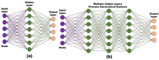
Figure 1.
Schematic of (a) shallow neural network and (b) deep neural network.
2.2.1. One-Hot Encoding
Owing to the development of algorithms in machine learning, methods for dealing with various data types have been proposed. The types of training data are generally divided into categorical and numerical data. The ANN training process was conducted primarily based on numerical data. Therefore, categorical data had to be transformed into numerical data in the classification problem and was additionally used to train the ANN models. The one-hot encoding method is the most representative method used to encode categorical data into numeric data, encoding categorical data into binary vectors with a maximum of one valid value. In Figure 2, each column represents the category to which the sample data (property of fracturing fluid) belongs, representing the units containing “1” in each category of property of fracturing fluid.
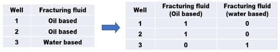
Figure 2.
Application of one-hot encoding for categorical variables.
2.2.2. Activation Functions
The activation function of a neural network has a significant influence on the predictive performance of the model. When the activation function is not used, the input of each node is a linear function of the output result of the node in the previous layer. In this case, regardless of the number of layers in the neural network, the output result is only a linear combination of the input, and the hidden layer is not considered for learning. The output result is no longer a linear combination of the input result only if the neural network model uses a nonlinear activation function. Table 1 shows five commonly used activation functions (i.e., linear, tanh, sigmoid, softplus and ReLU).

Table 1.
Mathematical expression of common activation functions.
2.2.3. Adam Optimization Algorithm
The adaptive momentum (Adam) optimization algorithm estimates the adaptive learning rate for all parameters involved in weight learning. It is a computationally efficient and very concise technique with a primary gradient with small memory requirements for the stochastic optimization process. This optimizer is used for DNN problems in high-dimensional spaces and huge datasets that calculate learning rates individually for various parameters from approximations containing first and second moments. The mathematical notation is as follows Equation (2).
where η is the initial learning rate, gt is the gradient at time t along ωj, xt is the exponential average of the gradient along ωj, yt is the exponential average of squares of gradient along ωj and is a small constant to avoid a zero denominator.
2.3. Principal Component Analysis
Data table X is first created in the form of m × n matrices by Equation (3). Furthermore, each row and column of X represents sample data and data categories, respectively. is an orthonormal matrix, where .
The newly calculated d can be calculated by Equation (4).
A subset of the data can be obtained by projecting to produce an r × k matrix. Y is defined by the following Equation (5).
The PCA algorithm is implemented in 5 steps. First, the average of the values in each column of the matrix is calculated and subtracted from all elements of that column. Second, calculating the covariance of the datasets. The covariance is a useful measure of the strength of relationships between different data categories or columns. The covariance for the data set itself is equal to the variance for that data set. Third, calculating the eigenvectors and eigenvalues of the squared covariance matrix: PC is arranged in decreasing order of the eigenvalues based on each eigenvector. The eigenvector or PC with the highest eigenvalues is called the first PC. The second major component follows until the last column. The data projected onto the first major component is of utmost importance. Fourth, the base vector is usually determined from the eigenvectors using a threshold applied to the eigenvalues. Lastly, the threshold has a direct impact on the preservation and calculation of important information. This is an essential process for calculating the principal component ratio.
where are n eigenvalues of covariance matrix C in descending order and is threshold. matrix Y is new data set of in the matrix X, in the eigenvector for W.
2.4. Variable Importance Analysis
The RF, GBM and XGBoost algorithms define two measures of variable importance analysis, as follows. Used to rank variables, for RF, the first measure is the rate of increase in the mean square error (%IncMSE) of the prediction for each tree, permutating out-of-bag data and The Gini Index (Equation (8)) is used to measure the quality of the partitioning (NodePurity) for all variables (nodes) in the tree. Whenever a node is split in a variable, the gini impurity for both child nodes is less than the parent node. Adding the gini reduction for each individual variable for every tree in the forest gives you a fast variable importance that is very consistent with the permutation importance measure. The higher the %IncMSE and IncNodePurity values, the more important the predictors. For GBM and XGBoost, the first indicator is calculated by the partial gain of each shape to the model based on the split total gain of this variable, and the second measure is the relative number of times the shape is used in the tree (frequency). The higher the gain and frequency ratio, the more important the predictor. Acquisition of the optimal subset of variables is a continuous search process and generally involves the following four steps [32]. The first step creates a subset. Second, the predictive performance of a subset of variables is evaluated. Third, the stop time of the variable search algorithm is determined. Lastly, it is used to verify the validity of the selected subset of variables.
where pi is the relative frequency of class i in Gini from C classes.
3. Dataset Preparation
The data used in this study come from shale reservoirs of the Montney Formation in Canada. The Lower Triassic Montney Formation is vastly wide, including about 130,000 km2. It also increases above 300 m from the west before starting outcrops in the Rocky Mountains. However, it is usually between 100 m and 300 m thick. As shown in Figure 3, most of the formations consist of siltstones that contain a small amount of sandstone originally collected at the bottom of a deep sea, while more porous sandstone and shell beds have been deposited in the shallow-water environment to the east. The depth of formation also generally increases from northeast to southwest with increasing reservoir pressure (5~20 kPa/m) and decreasing natural gas liquid (NGL) and oil content. In this region, volatile oil, gas condensate and dry gas zones are evenly distributed, and the main purpose of this study is to predict gas production.
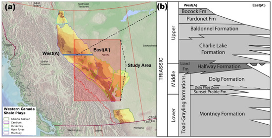
Figure 3.
Location of the 1239 shale gas wells used in this study.
The well data used in this study were extracted for 1239 horizontal wells from the geoSCOUT database system of geoLOGIC Systems Ltd. (Calgary, Alberta, Canada). There are 14 parameters in this study, the dependent variable to be predicted is 12 months cumulative gas production, and the number of independent variables is 13 (Table 2). In this study, 8 continuous variables were considered as input variables, of which true vertical depth, latitude (LAT), longitude (LON), continuous variable, well direction, well status and categorical variables are important variables that can replace geological factors. Previous studies predicting the production of shale reservoirs did not take into account geological factors [36,37]. It was assumed to be the same in the same formation. Due to the development characteristics of the shale reservoir (fast and intensive development process of numerous wells), it is impossible to obtain rock properties, porosity and permeability and reservoir pressure from all wells by performing both logging and well tests. Research was also carried out for the purpose of applying the coordinate well to replace or supplement geological factors [45,46,47]. In this study, a DNN model was developed that considers well direction and well status, which are categorical variables. The categorical parameters can be classified into three types: well status, completion and fracturing fluid. The independent variable had five categorical variables (Table 3). The first is the direction of the horizontal well. Horizontal drilling is performed in the opposite direction of the 90° or 270° azimuth to the minimum principal stress, which is an important rock mechanical property in horizontal well drilling of shale gas development. This is because it can improve the relevance of the more artificial fractures, and natural fractures are fractures in the opposite direction of the natural fractures or stress. Thus, it is an important factor in horizontal drilling. Well completion type is a factor that affects connectivity depending on the presence or absence of a casing when production occurs in the production zone of the reservoir. In the case of the technical group, it refers to the type of well completion technology in the case of multi-stage hydraulic fracturing. Ball and Seat cost is more than CT Cut/Port with packer installed. However, the initial production is known to be superior. Finally, four types of fracturing fluid are used: oil, slickwater, surfactant and water. Various fluids give more fracture pressure in the hydraulic fracturing process.
Table 2.
List of variables characteristics in the study datasets.
Table 3.
Data type and data counts of categorical variables.
To develop a data-driven deep learning model, eight additional independent variables were used. Table 4 shows summary statistics for data used as continuous variables (minimum, maximum, median and standard deviation). Standard deviation is an important variable used in standardization when creating a dataset. When creating a neural network-based machine learning model, a re-scaling process is performed to reduce the range of data. The purpose of normalization is, first, to not distort the difference between the ranges of values, and second, to change the values of the numeric columns in the data set to a common scale [48]. If the scale range is too large, noise data is generated, which increases the possibility of overfitting. It also causes the disappearance of connections between neurons through the activation function [49,50]. If the scales are different, the possibility of data characteristics being biased in one direction increases. In this study, data scaling was performed through the standardization of Equation (9).
where, z and are the standard score and is mean score, respectively. Xs is a score of datasets, is the standard deviation.
Table 4.
Summary statistics of numerical variables.
For continuous variables, true vertical depth (TVD), LAT and LON were used for the well type, which are important parameters to replace the well location and geological information. In the case of TVD, the minimum is 898 m to a maximum of 3863 m, and the location of the wells used in the DNN model is distributed from NW to SE. For the fracturing fluid and proppant, both the absolute amount and the amount injected per stage were used as independent variables. When hydraulic fracturing is performed, the two injected properties are considerably important factors. The standardization method is essential because the standard deviations of total fluid pumped (TFP) and total proppant placed (TPP) differ by more than 2 million gallons and 3 million pounds, respectively.
The response variable of primary interest in this study measures well cumulative gas production over a 12-month period (CGP12). The distribution of data and outliers was checked through EDA. Figure 4 shows the presence of outliers through a boxplot graph of typical four continuous variables (TPP, PPS, TFP, FPS). In the boxplot, the range of the box is the value of the first quartile (Q1) to the third quartile (Q3) when each variable is sorted in descending order. The value of the next Q3-Q1 is called the number of interquartile ranges (IQR) by the Equation (10).
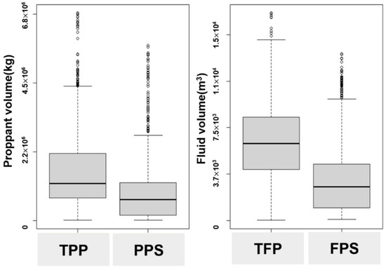
Figure 4.
A box plot analysis of hydraulic fracturing related parameters.
The thick line in the center of the box indicates the median value. The straight lines above and below the box are the minimum (minboxplot) and maximum values (maxboxplot). A point that deviates from the minimum and maximum values is an outlier.
An outlier is represented as a point if it is outside the minboxplot and maxboxplot values. For example, in Figure 4, the TPP variable has a minboxplot of 7.0 × 10³ and a maxboxplot value of 4.4 × 10⁶. The TPP values with higher than the maxboxplot were identified as outliers. As a boxplot result, outliers of 27 and 49 wells were found for TPP and TFP variables, respectively, which is 2.2% or 4.0% of the total data. Some outliers were also found in other parameters such as PPS and FPS, and a total of 96 wells were identified as outliers through box plots. Excluding duplicate well data, outliers for a total of 89 wells were identified. It was removed from the process of organizing training data. The above process is a preprocessing task to prevent overfitting of the supervised learning model.
Figure 5 visualizes the density of data distribution for each category of categorical variables and expresses the range of data distributed according to CGP12 using box plots and histograms. Figure 6 examines the pairwise scatter plot of the response to the predictor variable to determine which of the predictor variables has a significant effect on the response. This scatterplot matrix shows the relationship between all possible input and output variables. Using an empirical histogram of all variables along the diagonal. The figure also shows a positive or negative correlation between pairs of predictors. A positive relationship between CGP12, TPP (0.52), TFP (0.51) and stages (0.52) was confirmed in Figure 6 through the Pearson coefficient (R).
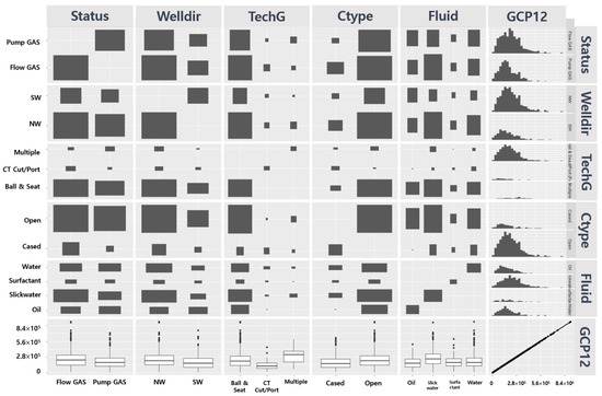
Figure 5.
Matrix plot showing the data distribution and histograms of categorical variables.
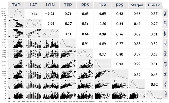
Figure 6.
Scatterplots showing the relationship between the parameters, histograms of numerical variables and Pearson correlation coefficient values.
Figure 7 shows the results of analyzing each pair of data in a 3D plot based on CGP12. Figure 7a show the cumulative production graph with the x-axis LON, y-axis LAT and z-axis CGP12, depending on the location of the well. This graph provides a visualization element to identify the potential for high production of the Montney Formation. The TPP vs. TFP showed a tendency for higher productivity as TPP and TFP volumes increase, except for some production wells (Figure 7b). In the case of stages vs. TVD, it was confirmed that the more stages, the deeper the TVD, and the higher the production (Figure 7c). Through a series of EDA, 1150 wells were selected as training data for the final DNN model, which was reduced by 89 from 1239 initial well training data.
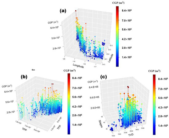
Figure 7.
3D plots graph of cumulative gas production over 12-months relationship to (a) longitude and latitude; (b) total proppant placed and total fluid pumped; (c) Stages and total vertical depth.
4. Process of Deep Learning Modeling
Figure 8 shows the analysis procedure of a production prediction model using data-driven supervised learning in shale and tight reservoirs applied hydraulic fracturing. The study was divided into six steps: (i) Step 1: data collection through the database system; (ii) Step 2: EDA (summary statistical analysis and visualization) for datasets; (iii) Step 3: variable importance analysis(various feature selection method); (iv) Step 4: selection of supervised learning algorithm and training process; (v) Step 5: production prediction; (vi) Step 6: improvement of predictive performance using sensitivity analysis for hyperparameters (retraining process back to Step 4).
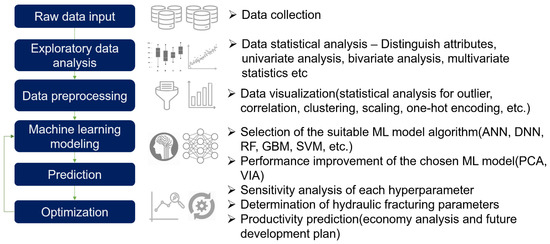
Figure 8.
Flow chart of machine learning modeling for production forecasting based on the data-driven approach.
STEP 1: Collect raw data from the database system and understand the data from domain knowledge.
STEP 2: Compute summary statistics using EDA techniques such as data exploration and univariate bivariate analysis. the datasets using various EDA visualization methods to determine data characteristics (preprocessing categorical and numerical variables) and perform outlier analysis, correlation to derive insights combined with domain knowledge.
STEP 3: Input features are selected through variable importance analysis (feature selection methods: Filtering, Wrapper and Embedded).
STEP 4: Select an appropriate supervised learning model (DNN, RF, GBM, SVM, etc.) and divide the training dataset into training, test and validation data, and extracts the characteristics of multivariate data through the principal component analysis.
STEP 5: Predict production using the generated model.
STEP 6: To improve the predictive performance of the generated model, perform a sensitivity analysis for hyperparameters or input variable optimization. Return to Step 4 and generate a model through retraining, iteratively as needed.
5. Results
In this work, we presented an open-source Python-based Keras deep learning application [51]. The 1150 wells in the database used in this study were analyzed using 70% training data (805 wells), 10% validation data (115 wells) and 20% test data (230 wells). To calculate and evaluate the error between a target variable and an estimated variable of the DNN model, the following three statistical parameters were used as measures: root mean square error (RMSE), mean absolute error (MAE) and mean absolute percentage error (MAPE) of Equations (14)–(16).
5.1. Principal Component Analysis
The principal components (PC) extracted through the PCA refer to variables that can explain the maximum variation (variance) in the entire data. The first principal component (PC 1) is extracted to have the maximum variance of the total (n) variable. The second principal component (PC 2) is extracted in an orthogonal relationship with the existing PC in order to reflect the fluctuations in the data that the PC1 could not explain to the maximum. In this way, up to the n-th PC’s can be calculated, and if all PC are used, the variance of the entire data can be explained. The PCA aims to minimize data information loss due to dimensionality reduction and uses fewer PC’s than the total number of variables. In general, the minimum number of PC’s is used based on 85% or more of the cumulative contribution rate. In Figure 9, the variables that have positive load on PC1 are PPS, TPP, TFP and FPS, and PC2 are Slick water, Ball and Seat, LAT and LON. Figure 10 shows the cumulative contribution rate of the variables of the sum of PC1 and PC2. The five variables in the order of TPP, PPS, Oil, TFP and FPS were found to have a cumulative 50% contribution rate. A production prediction model (PCA-DNN) was trained using a PC’s showing an 85% cumulative contribution rate, and compared with the previous PCA DNN model. The RMSE and MAPE of the test data of before PCA were 0.285 and 29.38%, respectively, and the RMSE and MAPE of the test data of after PCA were 0.229 and 24.47% (Table 5.)
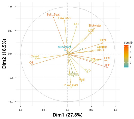
Figure 9.
Bi-plot using PC 1 and PC 2 scores.
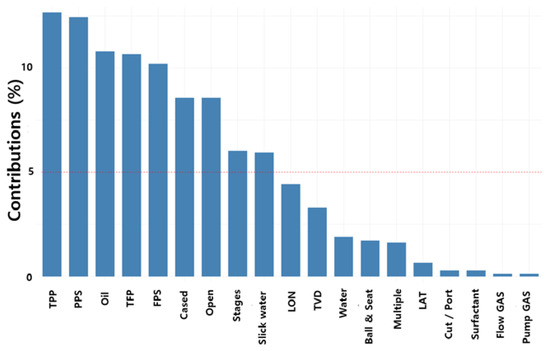
Figure 10.
The contribution of the variable of the sum of PC1 and PC2 to explain the variability in PCA.
Table 5.
Comparison of performance metrics of after principal component analysis.
5.2. Variable Importance Analysis
Figure 11 shows the results of the VIA of eight numerical parameters for cumulative gas production. The main effect of each parameter on cumulative gas production was applied to the tree-based RF, GBM, XGBoost algorithms and the average rank of three algorithms of variable importance analysis. The larger the bar graph value, the more important the parameter. In Figure 11a, the VIA of RF indicates that TVD and TFP are the most important parameters contributing to gas production volatility, with a relative impact of close to 100, followed by TPP and FPS. The GBM shows that TFP is the most important parameter and LON, TVD and TPP follow in that order (Figure 11b). For XGBoost, TPP was the most important variable, and TVD and TFP were confirmed to have significant impact also (Figure 11c).
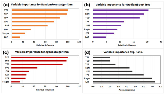
Figure 11.
Variable importance analysis by machine learning algorithms. (a) RF; (b) GBM; (c) XGBoost; (d) the value of average rank of variable importance of CGP for 12 months.
Figure 12 shows the comparison result of the 12 months cumulative gas production data and target data when the DNN model is trained through the input variable selected through VIA. Figure 12a is the comparison result of the learning materials of 805 wells. Figure 12b is the comparison result of 230 test data. It seems to have relatively high predictive performance through the cross plot. The RMSE and MAE of the training data ware 0.215 and 0.305, respectively, and the RMSE and MAE of the test data were 0.239 and 0.421 (Table 6).
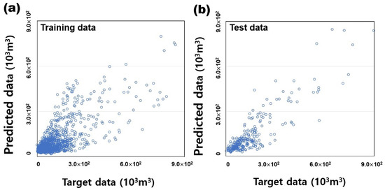
Figure 12.
Results of validation of training and test data for 12 months cumulative gas production. (a) training data; (b) test data.
Table 6.
Comparison of performance metrics of training and test data.
As a result of calculating the average rank of the previous VIA algorithm, it was found that TFP and TPP, which are important variables in hydraulic fracturing and well completion, are important parameters. In addition, it was confirmed that TVD and LON, which represent the location information of the well, are also variables with a relatively high influence. As a result of all comparative analyses, it can be seen that the relative importance of stages, which is the fracture interval, on cumulative gas production is low. The input variables of the DNN model selected as VIA (VIA-DNN) are TFP, TVD, TPP, LON, LAT and PPS. As a result of comparing the prediction performance of the six input variable training data and the entire model, the performance of both RMSE and MAPE is improved by about 20% (Table 7).
Table 7.
Comparison of performance metrics of after variable importance analysis.
5.3. Sensitivity Analysis for Hyperparameters
In this study, We performed hyperparameter sensitivity analysis using a Python-based Keras application. Among PCA-DNN and VIA-DNN, a sensitivity analysis was performed to study the effect of hyperparameters of the VIA-DNN model with excellent predictive performance on the prediction results and to further optimize the established DNN. There are 230 test wells used for sensitivity analysis comparison. Table 8 shows the range of each hyperparameter used for the sensitivity analysis. Figure 13 shows the effect of one-hot encoding to convert five categorical variables into binary vectors. When categorical variables were added to the DNN model as input variables (with one-hot encoding), it was found that the RMSE of 0.207 MAPE was 22.18%, and DNN models using only continuous variables had higher predictive performance than 0.242 MAPE of 26.14%. The key to the dropout method to prevent overfitting is to have some nodes in the DNN dropout with a dropout rate. Therefore, the dropout rate can significantly affect the training effect of the DNN. However, in this study, even if the dropout ratio increased from 10% to 40%, the learning result was not improved compared to the model without dropout. When the dropout ratio is 40%, as shown in Figure 14, the MAPE value differs by more than 5%. The activation function is an important parameter for calculating the relationship between the input data and output data of the DNN model. This can be seen as one of the discoveries that the activation function has greatly contributed to improving the predictive performance of the DNN model. In the case of the ReLU function, the MAPE was found to be at least 0.2% and at least 7.3% higher than the other four activation functions (linear, softplus, sigmoid, tanh). Therefore, ReLU was used in the DNN model (Figure 15a).
Table 8.
Hyperparameter sensitivity analysis range of DNN model.
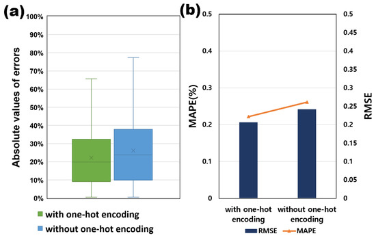
Figure 13.
One-hot encoding sensitivity analysis results of DNN models. (a) absolute error; (b) RMSE and MAPE.
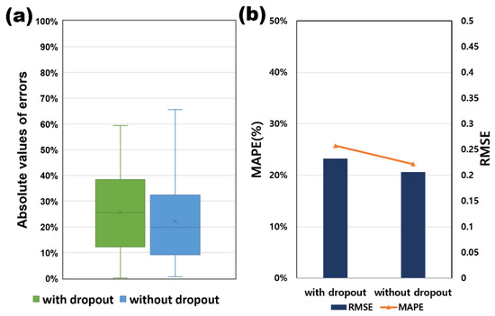
Figure 14.
Dropout method sensitivity analysis results of DNN models. (a) absolute error (b) RMSE and MAPE.
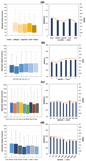
Figure 15.
Sensitivity analysis results for various hyperparameters. (a) activation function; (b) number of hidden layers; (c) number of neurons; (d) learning rate.
Figure 15b,c show the results of the sensitivity analysis of the number of hidden layers and the number of neurons in the hidden layers. When the number of hidden layer neurons increased to three or more, the predicted error gradually increased. The number of each neuron was assumed to be the same, and three hidden layer numbers were used in the previous results. As a result, the prediction error of 150 neurons was the lowest.
The loss function is a function of weights, and the learning rate determines the update speed of the weights in the DNN and determines the value of the loss function. If the learning rate is too large, the amount of weight change in one repetition increases, and if it is too small, the amount of change in weight becomes very small, resulting in slow learning speed and convergence to the local minimum. Therefore, there is an optimized learning rate for each DNN model. To determine the optimal learning rate, the value of the learning rate was compared with seven values between 0.0001 and 0.01. Figure 15d shows that the prediction absolute error increases when the learning rate is larger than 0.001. On the contrary, if the learning rate is lower than 0.001, the prediction absolute error is stable, but in conclusion, the learning rate 0.001 is the best result. Table 9 shows the optimal hyperparameter selection results calculated through the above sensitivity analysis.
Table 9.
Hyperparameter results of DNN model selected through sensitivity analysis.
5.4. Predictive Results of Test Wells Using DNN Model
Using a DNN model that selected the optimal hyperparameters in the sensitivity analysis, we performed a blind test on 4 wells that were not utilized for training out of 1150 test wells to compare and analyze the predicted performance in CGP12 prediction. Table 10 shows the test data used as input variables. The relative error between the actual value and the predicted value was at least 1.42% in test well 4 and 14.78% in test well 3 at the maximum (Table 11). As a result, the DNN model showed generally excellent predictive performance. Through the developed proxy model, it was found that hydraulic fracturing design can be designed, or production can be predicted. It can be modified when designing a field development plan for shale gas development.
Table 10.
Input parameters for four test wells.
Table 11.
Cumulative production predictive performance results for four test wells.
5.5. Comparison with Other Supervised Learning Algorithms
Figure 16 compares the predictive performance of the VIA-DNN, PCA-DNN, RF and SVM algorithms. Each model used 70% of the total data as training data and 10% as validation data, 20% as test data. The RMSE of the test data s was 0.233 for RF, 0.276 for SVM and 0.206 for the DNN. The MAPE indicated excellent predictive performance, with RF being 25.34%, SVM 29.74% and DNN 22.18%. Compared to the other two models, the CGP prediction model based on the DNN (VIA-DNN, PCA-DNN) performs better in the same test data.
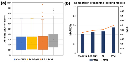
Figure 16.
Comparison of predictive performance for CGP prediction supervised learning models. (a) absolute error; (b) RMSE and MAPE.
6. Conclusions
In this study, we proposed a DNN-based production prediction method using the shale reservoirs datasets for Montney Formation. The datasets include both categorical and numerical variables based on data characteristics as well as hydraulic fracturing, well completion, well location and production operation data based on well characteristics. The main objective of this study is to provide a process for developing a proxy model using to predict the cumulative gas production of a shale reservoirs with multi-stage hydraulically fractured horizontal wells using data-driven deep learning algorithms. The results obtained through this study are summarized as follows.
Firstly, EDA was used to analyze data sets in a variety of ways, including outlier analysis, categorical and numeric variable analysis, and correlation analysis. This allows us to understand the structure and characteristics of the underlying data and can provide useful insights when generating DNN models. We eventually used 1150 as training data from 1239 wells through EDA.
Secondly, PCA is used to reduce the size of the input variable. It can also reduce the dimension of a wide variety of production-related input features, reduce the computational time of calculations and improve the accuracy of the model. In this study, we found that the cumulative contribution to PC was greater than 50% in hydraulic fracturing and well completion variables such as TPP, PPS, TFP and FPS. After PCA, in the case of the DNN model, the MAPE improved by about 4.91% compared to the original DNN model.
Third, the independent variables that have a high impact on CGP12 prediction were identified using VIA based on RF, GBM and XGBoost algorithms. This calculated the average importance ranking of the variables. The results show that the key parameters of total fluid pumping volume, total propane placement volume and completion in hydraulic fracture are important parameters. As a result of all comparative analyses, it was determined that the relative importance of the stages variable, which is the fracture stage spacing, on the cumulative gas production is reduced. The proposed model that removed the input variable through VIA showed that the MAPE improved by about 5.24% compared to the DNN model before the removal of input variable.
Lastly, hyperparameter sensitivity analysis is performed to create DNN models with better predictive performance. It was shown that applying one-hot encoding and not applying the dropout method improved the predictive performance of the DNN model. Furthermore, when the number of hidden layers is three, the absolute error chosen as the objective function for the test data is minimized. The number of neurons in each hidden layer was 150, the activation function was ReLU, and finally, the learning rate was 0.002. These parameters should be performed a sensitivity analysis before applying the DNN model to production forecasts due to exert a significant impact on the accuracy of the data-based model.
The proposed approach in this study is a very useful proxy model for reservoir engineers to plan future production forecasts and analyze economics in future development of nearby reservoirs. Future research will try to improve the workflow by using various additional input functions and data of other formations. In addition, we are trying to apply a deep learning algorithm (e.g., Long short term memory: LSTM, convolutional neural network—recurrent neural network: C-RNN) to a time series prediction problem that can predict future production profiles.
Author Contributions
Conceptualization, D.H. and S.K.; methodology, D.H.; software, D.H.; validation, D.H.; formal analysis, D.H. and S.K.; investigation, D.H.; resources, D.H.; data curation, D.H.; writing—original draft preparation, D.H.; writing—review and editing, D.H. and S.K.; visualization, D.H.; supervision, D.H.; project administration, D.H. and S.K.; funding acquisition, D.H. and S.K. All authors have read and agreed to the published version of the manuscript.
Funding
This work was supported by Institute of Information and communications Technology Planning and Evaluation (IITP) grant funded by the Korea government (MSIT) (2019-0-01561-002, Development and Application of Artificial Intelligence Techniques for Geospatial Information Analysis) and then supported by the National Research Foundation of Korea (NRF) grant funded by the Korea government (MSIT) (No. 2020R1I1A1A01060571).
Institutional Review Board Statement
Not applicable.
Informed Consent Statement
Not applicable.
Data Availability Statement
Not applicable.
Conflicts of Interest
The authors declare no conflict of interest.
Nomenclature
| ai | Weighted combination output of the i-th neuron |
| wi | Interconnection weight between the i-th neuron and j-th neuron |
| xi | Input data |
| bi | Bias of the i-th neuron of the n-th hidden layer |
| Initial learning rate | |
| xt | Exponential average of gradient along j |
| yt | Exponential average of square of gradient along j |
| gt | Gradient at time t along j |
| Constant number to avoid a zero denominator | |
| X | Matrix before transformation with principal component analysis |
| r | Column of matrix of initial datasets |
| c | Row of matrix of initial datasets |
| W | Orthogonal matrix in euclidean space |
| k | Row of matrix transformed by principal component analysis |
| Y | Matrix transformed by principal component analysis |
| Δ | Weight change momentum of adam optimizer |
| n eigenvalues of covariance matrix | |
| Threshold of n eigenvalues of covariance matrix C in descending order | |
| pi | Ratio of class i in the node whose gini index |
| c | Class of random forest node |
| z | Standardization score (z-score) |
| Xs | Score of dataset |
| Mean of dataset | |
| Standard deviation | |
| Minimum values of boxplot graph | |
| Maximum values of boxplot graph | |
| Observation point outside Q1 or Q3±1.5ⅹIQR in boxplot | |
| Xp | Predicted data |
| Actual data |
Abbreviations
| Abbreviation | Full Name |
| ANN | Artificial neural network |
| CART | Classification and regression tree |
| CGP12 | Cumulative gas production of 12 month (103 m3) |
| Ctype | Completion type |
| DNN | Deep neural network |
| EDA | Exploratory data analysis |
| EUR | Estimated ultimate recovery |
| Fluid | Base fracturing fluid |
| FPS | Average fluid pumped per stage (m3) |
| GBM | Gradient Boosting tree Machines |
| IQR | Interquartile range |
| LAT | Latitude |
| LON | Longitude |
| MAE | Mean absolute error |
| MAPE | Mean absolute percentage error (%) |
| PC | Principal component |
| PCA | Principal component analysis |
| PPS | Average proppant placed per stage (kg) |
| RF | Random forest |
| RMSE | Root mean square error |
| Q1 | First quartile |
| Q3 | Third quartile |
| Status | Well status |
| SVM | Support vector machine |
| TehcG | Completion technology group |
| TFP | Total fluid pumped (m3) |
| TPP | Total proppant placed (kg) |
| TVD | True vertical depth(m) |
| VIA | Variable importance analysis |
| Welldir | Well direction |
References
- Xu, B.; Haghighi, M.; Cooke, D.A.; Li, X. Production Data Analysis in Eagle Ford Shale Gas Reservoir. In Proceedings of the SPE/EAGE European Unconventional Resources Conference and Exhibition, Vienna, Austria, 20–22 March 2012. [Google Scholar] [CrossRef]
- Ding, D.Y. Numerical Simulation of Low Permeability Unconventional Gas Reservoirs. Presented at the SPE/EAGE European Unconventional Resources Conference and Exhibition, Vienna, Austria, 25–27 February 2014. [Google Scholar] [CrossRef]
- Al-Alwani, M.A.; Britt, L.K.; Dunn-Norman, S.; Alkinani, H.H.; Al-Hameedi, A.T.; Al-Attar, A.M. Review of Stimulation and Completion Activities in the United States Shale Plays. Paper ARMA 19-2003. Presented at the 53rd US Rock Mechanics/Geomechanics Symposium, New York, NY, USA, 23–26 June 2019. [Google Scholar] [CrossRef]
- Myers, R.R.; Knobloch, T.S.; Jacot, R.H.; Ayers, K.L. Production Analysis of Marcellus Shale Well Populations Using Public Data: What Can We Learn from The Past? In Proceedings of the SPE Eastern Regional Meeting, Lexington, KY, USA, 4–6 October 2017. [Google Scholar] [CrossRef]
- Wu, M.L.; Ding, M.C.; Yao, J.; Li, C.; Huang, Z.; Xu, S. Production-Performance Analysis of Composite Shale-Gas reservoirs by the Boundary-Element Method. SPE Reserv. Eval. Eng. 2018, 22, 238–252. [Google Scholar] [CrossRef]
- Sun, S.H.; Zhou, M.H.; Lu, W.; Davarpanah, A. Application of Symmetry Law in Numerical Modeling of Hydraulic Fracturing by Finite Element Method. Symmetry 2020, 12, 1122. [Google Scholar] [CrossRef]
- Sun, H.; Chawathe, A.; Hoteit, H.; Shi, X.; Li, L. Understanding Shale Gas Flow Behavior Using Numerical Simulation. SPE J. 2015, 20, 142–154. [Google Scholar] [CrossRef]
- Zhang, M.; Sun, Q.; Ayala, L.F. Semi-Analytical Modeling of Multi-Mechanism Gas Transport in Shale Reservoirs with Complex Hydraulic-Fracture Geometries by the Boundary Element Method. In Proceedings of the SPE Annual Technical Conference and Exhibition, Calgary, AB, Canada, 30 September–2 October 2019. [Google Scholar] [CrossRef]
- Davarpanah, A.; Shirmohammadi, R.; Mirshekari, B.; Aslani, A. Analysis of hydraulic fracturing techniques: Hybrid fuzzy approaches. Arab. J. Geosci. 2019, 12, 402. [Google Scholar] [CrossRef]
- Arps, J.J. Analysis of decline curves. Trans. Am. Inst. Min. Metall. Eng. 1945, 160, 228–247. [Google Scholar] [CrossRef]
- Tugan, M.F.; Weijermars, R. Improved EUR prediction for multi-fractured hydrocarbon wells based on 3-segment DCA: Implications for production forecasting of parent and child wells. J. Pet. Sci. Eng. 2020, 187, 106692. [Google Scholar] [CrossRef]
- Tugan, M.F.; Weijermars, R. Variation in b-sigmoids with flow regime transitions in support of a new 3-segment DCA method: Improved production forecasting for tight oil and gas wells. J. Pet. Sci. Eng. 2020, 192, 107243. [Google Scholar] [CrossRef]
- Varma, S.; Tabatabaie, S.H.J.; Ewert, J.L.; Mattar, L. Variation of hyperbolic-b-parameter for unconventional reservoirs and 3-segment hyperbolic decline. In Proceedings of the SPE/AAPG/SEG Unconventional Resources Technology Conference, Houston, TX, USA, 23–25 July 2018. [Google Scholar] [CrossRef]
- Valkó, P.P. Assigning value to stimulation in the barnett shale: A simultaneous analysis of 7000 plus production histories and well completion records. In Proceedings of the SPE Hydraulic Fracturing Technology Conference, The Woodlands, TX, USA, 19–21 January 2009. [Google Scholar] [CrossRef]
- Ilk, D.; Rushing, J.A.; Perego, A.D.; Blasingame, T.A. Exponential vs. Hyperbolic decline in tight gas sands: Understanding the origin and implications for reserve estimates using arps’ decline curves. In Proceedings of the SPE Annual Technical Conference and Exhibition, Denver, CO, USA, 21–24 September 2008. [Google Scholar] [CrossRef]
- Duong, A.N. Rate-decline analysis for fracture-dominated shale reservoirs. SPE Reserv. Eval. Eng. 2011, 14, 377–387. [Google Scholar] [CrossRef]
- Clark, A.J.; Lake, L.W.; Patzek, T.W. Production forecasting with logistic growth models. In Proceedings of the SPE Annual Technical Conference and Exhibition, Denver, CO, USA, 30 October–2 November 2011. [Google Scholar] [CrossRef]
- Hu, Y.; Weijermars, R.; Zuo, L.; Yu, W. Benchmarking EUR estimates for hydraulically fractured wells with and without fracture hits using various DCA methods. J. Pet. Sci. Eng. 2018, 162, 617–632. [Google Scholar] [CrossRef]
- Kulga, B.; Artun, E.; Ertekin, T. Development of a data-driven forecasting tool for hydraulically fractured, horizontal wells in tight-gas sands. Comput. Geosci. 2017, 103, 99–110. [Google Scholar] [CrossRef]
- Amini, S.; Mohaghegh, S. Application of Machine Learning and Artificial Intelligence in Proxy Modeling for Fluid Flow in Porous Media. Fluids 2019, 4, 126. [Google Scholar] [CrossRef]
- Kim, K.; Choe, J. Hydraulic Fracture Design with a Proxy Model for Unconventional Shale Gas Reservoir with Considering Feasibility Study. Energies 2019, 12, 220. [Google Scholar] [CrossRef]
- Knudsen, B.R.; Foss, B. Designing shale-well proxy models for field development and production optimization problems. J. Nat. Gas Sci. Eng. 2015, 27 Pt 2, 504–514. [Google Scholar] [CrossRef]
- Weijermars, R.; Tugan, M.F.; Khanal, A. Production rates and EUR forecasts for interfering parent-parent wells and parent-child wells: Fast analytical solutions and validation with numerical reservoir simulators. J. Pet. Sci. Eng. 2020, 190, 107032. [Google Scholar] [CrossRef]
- Weijermars, R.; Nandlal, K.; Tugan, M.F.; Dusterhoft, R.; Neil, S. Wolfcamp Hydraulic Fracture Test Site Drained Rock Volume and Recovery Factors Visualized by Scaled Complex Analysis Method (CAM): Emulating Multiple Data Sources (Production Rates, Water Cuts, Pressure Gauges, Flow Regime Changes, and b-Sigmoids). In Proceedings of the SPE/AAPG/SEG Unconventional Resources Technology Conference, Virtual, 20–22 July 2020. [Google Scholar] [CrossRef]
- Tugan, M.F.; Sinayuc, C. A new fully probabilistic methodology and a software for assessing uncertainties and managing risks in shale gas projects at any maturity stage. J. Pet. Sci. Eng. 2018, 168, 107–118. [Google Scholar] [CrossRef]
- Mohaghegh, S.D. Reservoir Modeling of Shale Formations. J. Nat. Gas Sci. Eng. 2013, 12, 22–33. [Google Scholar] [CrossRef]
- Han, D.; Jung, J.; Kwon, S. Comparative Study on Supervised Learning Models for Productivity Forecasting of Shale Reservoirs Based on a Data-Driven Approach. Appl. Sci. 2020, 10, 1267. [Google Scholar] [CrossRef]
- Bansal, Y.; Ertekin, T.; Karpyn, Z.; Ayala, L.; Nejad, A.; Suleen, F.; Balogun, O.; Sun, Q. Forecasting Well Performance in a Discontinuous Tight Oil Reservoirs Using Artificial Neural Networks. In Proceedings of the SPE Unconventional Resources Conference, Woodlands, TX, USA, 10–12 April 2016. [Google Scholar] [CrossRef]
- Zhong, M.; Schuetter, J.; Mishra, S.; Lafollette, R.F. Do data mining methods matter? A Wolfcamp Shale case study. In Proceedings of the SPE Hydraulic Fracturing Technology Conference and Exhibition, Woodlands, TX, USA, 3–5 February 2015. [Google Scholar] [CrossRef]
- Lolon, E.; Hamidieh, K.; Weijers, L.; Mayerhofer, M.; Melcher, H.; Oduba, O. Evaluating the Relationship Between Well Parameters and Production Using Multivariate Statistical Models: A Middle Bakken and Three Forks Case History. In Proceedings of the SPE Hydraulic Fracturing Technology Conference, Woodlands, TX, USA, 9–11 February 2016. [Google Scholar] [CrossRef]
- Bowie, B. Machine Learning Applied to Optimize Duvernay Well Performance. In Proceedings of the SPE Canada Unconventional Resources Conference, Calgary, AB, Canada, 13–14 March 2014. [Google Scholar] [CrossRef]
- Alabboodi, M.J.; Mohaghegh, S.D. Conditioning the Estimating Ultimate Recovery of Shale Wells to Reservoir and Completion Parameters. In Proceedings of the SPE Eastern Regional Meeting, Canton, OH, USA, 13–15 September 2016. [Google Scholar] [CrossRef]
- Mohaghegh, S.D.; Gaskari, R.; Maysami, M. Shale Analytics: Making Production and Operational Decisions Based on Facts: A Case Study in Marcellus Shale. In Proceedings of the SPE Hydraulic Fracturing Technology Conference, Woodlands, TX, USA, 24–26 January 2017. [Google Scholar] [CrossRef]
- Li, Y.; Han, Y. Decline Curve Analysis for Production Forecasting Based on Machine Learning. In Proceedings of the SPE Symposium: Production Enhancement and Cost Optimization, Kuala Lumpur, Malaysia, 7–8 November 2017. [Google Scholar] [CrossRef]
- Han, D.; Kwon, S.; Son, H.; Lee, J. Production Forecasting for Shale Gas Well in Transient Flow Using Machine Learning and Decline Curve Analysis. In Proceedings of the SPE/AAPG/SEG Asia Pacific Unconventional Resources Technology Conference, Brisbane, Australia, 18–19 November 2019. [Google Scholar] [CrossRef]
- Rahmanifard, H.; Alimohamadi, H.; Ian, G. Well Performance Prediction in Montney Formation Using Machine Learning Approaches. In Proceedings of the SPE/AAPG/SEG Unconventional Resources Technology Conference, Virtual, 20–22 July 2020. [Google Scholar] [CrossRef]
- Sheikhi, G.Y.; Mehdi, G. Machine Learning Interpretability Application to Optimize Well Completion in Montney. In Proceedings of the SPE Canada Unconventional Resources Conference, Virtual, 28 September 2020. [Google Scholar] [CrossRef]
- Wang, S.; Chen, S. Insights to fracture stimulation design in unconventional reservoirs based on machine learning modeling. J. Pet. Sci. Eng. 2019, 174, 682–695. [Google Scholar] [CrossRef]
- Mahta, V.; Ian, G. On multistage hydraulic fracturing in tight gas reservoirs: Montney Formation, Alberta, Canada. J. Pet. Sci. Eng. 2019, 174, 1127–1141. [Google Scholar] [CrossRef]
- Makinde, I.; Lee, W.J. Principal components methodology—A novel approach to forecasting production from liquid-rich shale (LRS) reservoirs. Petroleum 2019, 5, 227–242. [Google Scholar] [CrossRef]
- Khanal, A.; Khoshghadam, M.; Lee, W.J.; Nikolaou, M. New forecasting method for liquid rich shale gas condensate reservoirs with data driven approach using principal component analysis. J. Nat. Gas Sci. Eng. 2017, 38, 621–637. [Google Scholar] [CrossRef]
- Tukey, J.W. Exploratory Data Analysis; Pearson: London, UK, 1977; ISBN 978-0201076165. [Google Scholar]
- LeCun, Y.; Bengio, Y.; Hinton, G. Deep learning. Nature 2015, 521, 436–444. [Google Scholar] [CrossRef] [PubMed]
- Dash, M.; Liu, H. Feature selection for classification. Intell. Data Anal. 1997, 1, 131–156. [Google Scholar] [CrossRef]
- Lafollette, R.F.; Holcomb, W.D.; Jorge, A. Impact of Completion System, Staging, and Hydraulic Fracturing Trends in the Bakken Formation of the Eastern Williston Basin. In Proceedings of the SPE Hydraulic Fracturing Technology Conference, Woodlands, TX, USA, 6–8 February 2012. [Google Scholar] [CrossRef]
- Gullickson, G.; Fiscus, K.; Peter, C. Completion Influence on Production Decline in the Bakken/Three Forks Play. In Proceedings of the SPE Western North American and Rocky Mountain Joint Meeting, Denver, CO, USA, 16–18 April 2014. [Google Scholar] [CrossRef]
- Schuetter, J.; Mishra, S.; Zhong, M.; Randy, L. Data Analytics for Production Optimization in Unconventional Reservoirs. In Proceedings of the SPE/AAPG/SEG Unconventional Resources Technology Conference, San Antonio, TX, USA, 20–22 July 2015. [Google Scholar] [CrossRef]
- Mustafa, A.N.; Moustafa, E.; Abdelsalam, A.S. Artificial neural network application for multiphase flow patterns detection: A new approach. J. Pet. Sci. Eng. 2016, 145, 548–564. [Google Scholar] [CrossRef]
- Shengwei, Z.; Konstantinos, A. Evaluation of standardized and study-specific diffusion tensor imaging templates of the adult human brain: Template characteristics, spatial normalization accuracy, and detection of small inter-group FA differences. NeuroImage 2018, 172, 40–50. [Google Scholar] [CrossRef]
- Hongyan, Y.; Reza, R.; Zhenliang, W.; Tongcheng, H.; Yihuai, Z.; Muhammad, A.; Lukman, J. A new method for TOC estimation in tight shale gas reservoirs. Int. J. Coal Geol. 2017, 179, 269–277. [Google Scholar] [CrossRef]
- Chollet, F. Keras. 2015. Available online: https://keras.io (accessed on 15 June 2021).


Publisher’s Note: MDPI stays neutral with regard to jurisdictional claims in published maps and institutional affiliations. |
© 2021 by the authors. Licensee MDPI, Basel, Switzerland. This article is an open access article distributed under the terms and conditions of the Creative Commons Attribution (CC BY) license (https://creativecommons.org/licenses/by/4.0/).