Abstract
With the increasing trend toward the miniaturization of electronic devices, the issue of heat dissipation becomes essential. The use of phase changes in a two-phase closed thermosyphon (TPCT) enables a significant reduction in the heat generated even at high temperatures. In this paper, we propose a modification of the evaporation–condensation model implemented in ANSYS Fluent. The modification was to manipulate the value of the mass transfer time relaxation parameter for evaporation and condensation. The developed model in the form of a UDF script allowed the introduction of additional source equations, and the obtained solution is compared with the results available in the literature. The variable value of the mass transfer time relaxation parameter during condensation r depending on the density of the liquid and vapour phase was taken into account in the calculations. However, compared to previous numerical studies, more accurate modelling of the phase change phenomenon of the medium in the thermosyphon was possible by adopting a mass transfer time relaxation parameter during evaporation r = 1. The assumption of ten-fold higher values resulted in overestimated temperature values in all sections of the thermosyphon. Hence, the coefficient r should be selected individually depending on the case under study. A too large value may cause difficulties in obtaining the convergence of solutions, which, in the case of numerical grids with many elements (especially three-dimensional), significantly increases the computation time.
1. Introduction
Despite the impressive advances that have been made in recent years regarding the cooling of electronic systems, the removal of high heat fluxes from high-tech devices is undoubtedly complex and, in some cases, inadequate. The choice of a proper cooling method for electronic systems depends on many factors: the power density and its magnitude, the size of the overall device and its components, the operating environment, and economic aspects.
The simplest division of cooling mechanisms divides them by the state of aggregation of the working medium [1]. The following distinction can be made:
- cooling systems in which the medium does not change its physical state during operation—this can be air, water, or other fluids; and
- techniques using a phase change of the working medium.
In the process of heat transfer in a cooling system, convection plays the most important role, and the measure of its intensity is determined by the heat transfer coefficient h. The value of this parameter can range from several to even several hundred thousand [2,3]. Many fluids have their applications in cooling electronic instruments, of which water proves to be the most effective [4]. By taking additional advantage of its phase change, high values of heat transfer coefficients can be obtained [5].
A thermosyphon is a component that significantly improves heat transfer in electronic devices. Unlike a heat pipe with porous structures, in a thermosyphon, the working medium is returned only by gravitational forces [2]. Therefore, this element should be vertically located. It is also worth noting that the evaporator is located below the condensing section [6]. The heat input in the evaporator forces the movement of the vapour core toward the condenser, where the fluid is condensed [7].
An essential operating parameter of a heat pipe is thermal resistance. It turns out that its value is influenced, among other things, by the bending angle. The results of research conducted by Chen [8] demonstrated that, by increasing the bending angle from 0 °C to 90 °C (i.e., changing from the horizontal to the vertical position), it was possible to decrease the value of thermal resistance from 0.6207 to 0.1885 K/W. A simulation carried out by Fadhl [9] showed that the thermal resistance value also decreased with increasing the fill ratio. An increase in the filling ratio from 0.3 to 1 reduced the temperature difference between the evaporator and condenser walls and, consequently, thermal resistance.
There are many potential applications for phase change in heat pipes. For example, a pulsating heat pipe operating with a graphene-water ethylene glycol nano-suspension can be used for low-temperature heat recovery [10]. Furthermore, there are studies [11] on applying different working mediums, including n-pentane-acetone and n-pentane-methanol mixtures. The experimental results presented in this paper showed that both the fill ratio and the tilt angle were key parameters affecting the system’s thermal performance.
The dispersion of nanoparticles in base fluids can also be used to improve the thermal properties of working mediums. To this purpose, experimental studies have been performed to investigate the problem of the fouling formation [12], and numerical calculations were carried out to determine more accurate values of the thermal conductivity of CuO (II)/water nanofluid [13]. The great importance of performing research on phase change cooling systems was also confirmed by the possibility of improving heat transfer by applying a magnetic field to the kerosene/Fe2O3 nanofluid in a copper oscillating heat pipe [14].
It is also worthwhile to look at the development of numerical codes for solving thermal-fluid problems in thermosyphons. Back in the early 2000s, Basran and Kücüka [15] studied a two-dimensional geometric model of a vertical, closed heat pipe. They defined the heat source and heat removal on the walls of the evaporator and condenser sections using constant temperatures. They showed that the numerical model was adequate for estimating heat transfer in a thermosyphon. While still in the early stages of the development of commercial numerical codes, Liu, Li, and Chen [16] conducted numerous studies to understand the properties of thermosyphons and the effects of various parameters on their performance.
Legierski and Więcek [17] were among the first to apply commercial CFD codes to heat pipe studies. In their work, they included a horizontal heat pipe connecting two tanks. The first, filled with hot water, was connected to the evaporator, while the cool water tank was in contact with the condenser. By implementing user-defined functions (UDF), the evaporator and condenser wall temperatures were updated throughout the simulation. These studies did not consider the phase change of the medium; however, they provided a source of knowledge about the value of the effective thermal conductivity coefficient of the system under study. The simulations resulted in coefficients in the range of 15,000 to 30,000 W/(mK) [17], which is in agreement with the data reported in the literature by the authors of the publication. The simplified numerical studies of the thermosyphon, neglecting the phase change, were carried out by Ramalingam [18].
A huge step in modelling the evaporation and condensation of the working medium in a thermosyphon was the use of Lee’s model [19]. This is currently implemented in ANSYS Fluent and available under the name evaporation–condensation. A simple temperature differencing scheme was used to calculate the mass source terms during evaporation and condensation, which was shown to agree with the experimental data.
The mass transfer equations for evaporation process (T1 > T) have the form [20]:
Similarly, for the condensation process (T < T), the relations can be written as follows:
The Equations (1)–(4) include the coefficient r and r, which is a measure of the intensity of the mass transfer in the evaporation and condensation processes. It is recommended that their value be such to keep the saturation temperature reasonably close to the saturation temperature and to avoid divergence problems. As an empirical coefficient, r and r have different values for different problems. It can be determined from Equations (5) and (6) that [21]:
In the evaporation–condensation model, these are equal to 0.1 1/s.These values were adopted in numerical studies of boiling in serpentine-shaped pipes [22], in the two-phase flow of diesel fuel [23], and in the evaporation and condensation process of a hydrocarbon feedstock in a horizontal heat pipe [20]. The constant values of the r = 0.1 and the r = 0.1 were also adopted by Alizadehdakhel [24] to investigate the effect of the heat input and fill ratio on thermosyphon performance.
In contrast, Lin and Wang [25] simulated the heat transfer mechanism in miniature oscillating heat pipes. To study the two-phase flow behaviour taking place vertically, they proposed their own mathematical and physical model. The simulation used the VOF phase change model in combination with the relations derived by De Schepper [20], which were implemented through UDF. A Continuum Surface Force (CSF) model was used to account for the effect of surface tension. A time-lapse simulation of 60 s was performed to compare the flow visualization with images taken during the experimental study. The analysis predicted the appearance of oscillations of similar frequency in both the condenser and evaporator sections. In addition, the study showed that decreasing diameter positively affected the thermal performance of the thermosyphon.
Fadhl also conducted a study of a cooling system using a thermosyphon. In his work [26], he applied a VOF model using source terms introduced by defined functions. He successfully reproduced the phenomenon of water changing its physical state from liquid to vapour. A two-dimensional geometric model of a 500-mm long thermosyphon was performed. The length of the evaporator, adiabatic, and condenser sections were 200, 100, and 200 mm, respectively. Compared to previous studies, he introduced the dependence of the surface tension coefficient between the liquid and vapour phases as a temperature-dependent variable in the thermosyphon. He assumed a saturation temperature of 373.15 K, which corresponds to an operating pressure prevailing in the thermosyphon equal to atmospheric pressure. Fadhl also ran similar analyses using R134a and R404a [27], and performed studies on a three-dimensional geometric model of the thermosyphon [9].
A similar study was performed by Zhang [28]. He simulated a two-dimensional thermosyphon with a length of 250 mm and an inner diameter of 8.32 mm. He used identical types of boundary conditions as Fadhl. He assumed a heat input of 40, 60, and 80 W; however, his work did not specify the coolant temperature and heat transfer coefficient values. Compared with Fadhl’s study, he lowered the saturation temperature of water to 308.55 K and also reduced the time step of the transient simulation from 0.0005 [26] to 0.0001 s. He took the value of the fill ratio equal to 0.6. As a result of the simulations, he obtained very accurate calculation results compared to those obtained in his experiment.
However, the values of coefficient r and r need not always be 0.1 1/s, as in the cases mentioned above. In other studies [29,30], values equal to 100 1/s were assumed. CFD analysis of water droplet evaporation under atmospheric conditions [31], on the other hand, required a much smaller value of this coefficient—in the range of 0.001–0.04 1/s. On the contrary, in simulations of the evaporation process performed by Das [32], the optimal value of the mass transfer time relaxation parameter during evaporation and condensation was in the range of 0.3–0.9 1/s. Numerical experiments determined this coefficient because it depends on local thermodynamic conditions, humidity, and other numerical and model parameters.
In a numerical study of thermosyphons, Xu [33] adopted four different values of r and r 0.8; 0.9; 0.95; and 1 1/s. This reduced the error in determining the temperature distribution by an average of 2% compared to using the evaporation–condensation model. It was also possible to significantly reduce the error in the thermal resistance values. On the other hand, in Kafeel’s simulations [34], the values of the relaxation coefficient for evaporation were 0.09; 0.3; and 0.5 1/s, while for condensation, the value of the relaxation coefficient was calculated from the mass transfer rate during evaporation. The study found that an increase in the mass transfer time relaxation parameter during evaporation resulted in a decrease in the overall thermosyphon temperature due to the increased evaporation rate of the working fluid. In a subsequent publication, [35], the value of r was taken as 0.1, while r was determined in a similar way as in the work [34].
The studies of oscillating heat pipes by Wang [36] are also noteworthy. He also used Lee’s model in analysing the phase change of the working medium. In the first case, the values of the mass transfer time relaxation parameters during evaporation and condensation remained unchanged at 0.1 1/s. In the second variant, these coefficients were 0.1 and 973.356 1/s; in the third 1 and 9733.56 1/s; and in the fourth 10 and 97,335.6 1/s, respectively. These simulations allowed us to investigate the effects of the r and r coefficients on the resulting temperature distribution and thermal resistance values.
It turned out that the results of the CFD analysis most similar to experimental studies were achieved using the fourth variant of calculations. While the temperature values in the adiabatic and evaporator sections were largely convergent with each other, the temperature differences in the condenser for the first three cases were as high as several tens of degrees Celsius. Similar conclusions can be drawn from the analysis of the thermal resistance error. Relative to the experimental study, this error was 410% in case one, 203% in case two, 64% in case three, and 6% in case four.
A valuable numerical study of the thermosyphon was also realized by Kim [37]. He assumed a domain with identical dimensions as in Fadhl’s work and the same boundary conditions, fluid properties, and simulation parameters. However, he investigated the effect of the mass transfer time relaxation parameter during condensation (r), which had been constant in most papers. It turned out that during the simulation, its value varied from 0 to 100 1/s and depended both on the mass transfer time relaxation parameter during evaporation and on the liquid and vapour phase densities (Equation (7)).
By making the coefficient r dependent on these parameters, he obtained more accurate results for the average evaporator wall temperature.
Recent numerical studies included not only the development of the mathematical model but also the modification of the geometrical model of the thermosyphon by introducing fins [38], considering the working medium as methanol [39] or nanofluid [40] or studying the influence of boundary conditions [41].
The cited publications highlighted the need to modify Lee’s model to further investigate the phase change. Reducing the error between experimental and numerical simulation results was possible by manipulating the mass transfer time relaxation parameter values for both evaporation and condensation.
To the best of the authors’ knowledge, none of the studies considered the possibility of determining the value of coefficient r from Equation (7) while changing coefficient r from the Lee model’s default value of 0.1. The fact mentioned above motivated the authors to manipulate the value of the mass transfer time relaxation parameter for evaporation and condensation. Several works have confirmed that increasing this coefficient, especially for the evaporation process, is associated with a reduction in the error between simulation and experiment. Furthermore, the determination of the mass transfer time relaxation parameter during condensation as dependent on the liquid and vapour phase densities allows its value to depend on the simulation time. Hence, developing a modified computational model combining both relationships can contribute to more accurate CFD analysis results.
The objective of this work was to numerically investigate the impact of both the r and r values on the temperature distribution along the thermosyphon and the value of thermal resistance.The unmodified Lee model (Case 1) for the geometric model described in the articles [9,37] was used in the research on the thermosyphon. Then, based on this, three new computational models (Case 2, Case 3, and Case 4) were developed, in which the coefficient r takes the values of 0.1, 1, and 10 1/s, respectively. The value of coefficient r was made dependent on both the value of coefficient r and the density of the liquid and vapour fractions. Subsequently, the results obtained by the above models were compared with the results of CFD analysis by Fadhl [9], and Kim [37], as well as the experimental results [9].
2. Methodology
2.1. Computational Domain
Both the dimensions of the computational domain and the assumptions about the computational model were adopted from experimental studies developed by Fadhl [9]. In this experiment, the heat was injected into the system through the evaporator using a 500 W heater. A variable voltage transformer was used to control the electrical power supplied to the walls of the evaporator.
To minimize the heat loss to the environment, the author of the experiment wrapped the evaporator with layers of fire-proof and thermal insulation. Then, the walls of both the evaporator and the adiabatic sections were wrapped with layers of high-temperature thermal ceramic insulation. The heat was removed from the condenser section by a double pipe concentric heat exchanger. The working medium in the thermosyphon was water. Fadhl determined the characteristics of the thermosyphon based on the temperature values on the walls. Temperature measurement was carried out using thermocouples. Their arrangement is shown in Figure 1.
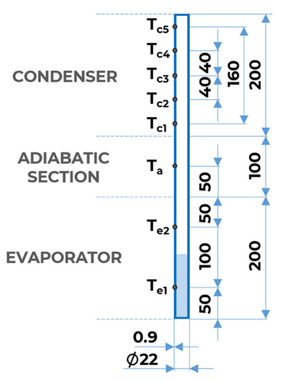
Figure 1.
Geometrical model of a closed thermosyphon.
Previous research [42,43] suggested designing the thermosyphon so that the evaporator section area is smaller than that of the condenser section. This makes it possible to generate a higher heat flux in the evaporator, increase the thermal driving force in the system and increase the efficiency of the thermosyphon. However, in order to compare experimental and numerical results, we decided to reproduce the geometric model described in the reference [9]. A two-dimensional geometric model of the thermosyphon was developed, representing its 500 × 22 mm cross-section (Figure 1). The lengths of the condenser, evaporator, and adiabatic sections were 200, 200, and 100 mm, respectively, while the width of the thermosyphon wall was 0.9 mm.
The geometric model, shown in Figure 2, was created using ANSYS Spaceclaim software. It consists of two internal areas, the top (fluid_up) and the bottom (fluid_down), which correspond to the working medium. The division was made because of the need to give these areas different initial conditions, with the height of the bottom section being equal to 50% of the height of the evaporator section. In contrast, the outer part of the domain is the wall of the thermosyphon.
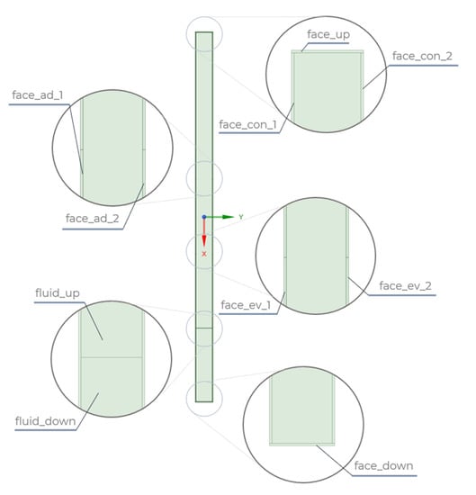
Figure 2.
Partitioning the geometric model of the thermosyphon into areas.
Similarly to the fluid, the division into different areas was also applied. The wall consists of the top and bottom surfaces (face_up, face_down), the adiabatic part (face_ad_1, face_ad_2), the area corresponding to the condenser (face_con_1, face_con_2), and the evaporator (face_ev_1, face_ev_2). Making this division further enabled the sections to be given different boundary conditions. At the geometric model creation stage, a share topology function was additionally assigned to the model to merge it to generate a consistent mesh.
2.2. Computational Model
2.2.1. Mathematical Model
In the developed system, there is heat transfer described as a function of spatial coordinates and time. Parallel fluid transport occurs in this case. In the model studied, heat is directed to the walls of the evaporator, where the conduction occurs, and then heat is transferred to the fluid, where the phase of the working medium changes. When considering the solid domain, heat transfer by convection was assumed to be neglected. Heat transport has been described by the Fourier–Kirchhoff equation [44].
Numerical solutions based on the finite volume method are much more difficult for multiphase flows than for single-phase flow. The reason for this is the existence of non-stationary interfaces between phases. In contrast, physical properties, such as density and viscosity, change at the surfaces connecting the two phases. The Volume of Fluid technique was used to model the phase change phenomenon of the working fluid by defining the motion of all phases and defining the motion of the interfaces.
This technique is used to model immiscible fluids with a clearly defined boundary. However, the method cannot be used to analyse two gases because they mix at the molecular level. This model allows analysis of, for example, two immiscible liquids, the separation of a liquid stream, or the motion of large bubbles in a liquid. In these cases, the assumption of a noticeably large interface length compared to the size of the computational domain must be satisfied [45].
The VOF model is based on the fact that each cell in the domain is occupied by one phase or a combination of two phases. In other words, if the volume fraction of liquid were defined by the value , while is the volume fraction of vapour, the following three conditions are possible:
- = 0; the cell is fully occupied by liquid;
- = 1; the cell is fully occupied by vapor,;
- 0 < < 1; the cell is located at the interface between the two phases.
For the third case, the following relation can be written:
The governing equations are used to describe the motion of a working fluid in a thermosyphon.
The continuity equation can be written by the expression [46]:
The solution of the above equation for the volume fraction for one of the phases is used to track the interfacial boundary. Thus, the continuity equation of the VOF model for the secondary phase (liquid) can be expressed as [47]:
An additional term S (mass source term) is used here and used to calculate the mass transfer during evaporation and condensation.
The presented continuity equation (Equation (11)) can be called the volume fraction equation. It is not solved for the primary phase (vapour) but only for the secondary phase (liquid). When a cell is not completely occupied by a primary phase or a secondary phase, a mixture of phases exists. Thus, the density of the mixture is given as the density averaged over the volume fractions and takes the following form [48]:
The forces acting in the system come from gravity, pressure, friction, and surface tension. To account for the effect of surface tension along the interface, the Continuum Surface Force (CSF) model proposed by Brackbill [49] was added to the momentum equation:
This equation takes into account additional coefficients, such as the surface tension and the surface curvature.
Considering the above forces, the momentum equation for the VOF model takes the form of [50]:
The average value of the dynamic viscosity can be calculated using the equation:
The energy equation for the VOF model has the following form [50]:
The source term for the energy equation (S) is used to calculate heat transfer during evaporation and condensation. The VOF model uses temperature as a mass-averaged variable, and thermal conductivity is calculated as:
The VOF model also approximates the value of internal energy (e) in the form:
In the equation, the values of e and e are based on specific heat (c and c) of the phase and common temperature determined by the equation of state:
The source terms S and S were introduced into the model using the Lee model. The mass source terms during evaporation and condensation for the liquid and vapour phases were shown in earlier discussions through Equations (1)–(4). In addition, the energy equations must be considered [20]:
In the Lee model studies, different values of r and r coefficients were implemented. Thus, the four cases described in Table 1 were examined.

Table 1.
Values of r and r for the given cases.
In order to solve Equations (11), (14) and (16), appropriate boundary conditions must be assumed. These are schematically shown in Figure 3. The top, bottom, and corresponding adiabatic section walls were assigned a zero heat flux density value. The third type boundary condition was assumed for the condenser walls, while a constant heat flux density value was specified for the evaporator walls. Values for average condenser temperature T, coolant temperature T, and heat flux in condenser section and evaporator section were taken in accordance with the experimental studies [9].
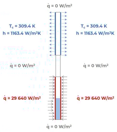
Figure 3.
Assigning boundary conditions to appropriate surfaces.
The heat transfer coefficient for the evaporator section was determined using Equation (23). For this purpose, the lateral area of the condenser section was determined A, and the coolant temperature value was calculated from the logarithmic mean of the temperature difference at the inlet and outlet of the tube. The heat flux density was calculated from the heat flux applied to the evaporator section (Equation (24)). This also depends on the area of the inner wall of the evaporator A, that is, the length of this section l and the inner diameter of the thermosyphon d.
Then, the properties of the phases involved in the modelled phenomenon were determined. It was assumed that two phases would be simulated: a primary phase—water vapour, and a secondary phase—liquid water. The density of liquid water was determined to be temperature-dependent. For this purpose, it was determined using a polynomial function. The most important properties are shown in Table 2.
Table 2.
Continuous and discrete phase properties [27].
The properties of copper, the material from which the walls of the thermosyphon were made, were also determined. These are shown in Table 3.
Table 3.
Properties of copper.
The Phase Interaction settings were also selected. The mechanism of mass transfer from the liquid to the vapour through the evaporation and condensation model developed by Lee (evaporation–condensation) was chosen. A constant saturation temperature of 373.15 K was determined.
The value of the surface tension coefficient between the liquid and vapour phases was also taken as a temperature-dependent value. It was determined using Equation (25) [27].
The working conditions of the domain were also defined. These are characterized by:
- operating pressure (p = 101,325 Pa); and
- average temperature in the domain (T = 298 K).
A pressure-based solver was used for the calculations. The type of phenomenon under study was set to transient. The effect of gravitational force was included in the calculation; the direction of gravitational acceleration was the same as the direction of the OX axis, and its value was taken as 9.81 m/s.
The explicit formulation of the multiphase model was adopted in the simulation, which differs from the implicit formulation in the type of equations solved in sub time steps. The first method functions as a default setting while allowing the use of the Geo-Reconstruct volume fraction discretization scheme, ensuring that a clear interface between phases is obtained and preventing the appearance of numerical diffusion.
The simulation uses the Implicit Body Force calculation formula to support calculations of cases characterized by, for example, the gravitational force acting on substances with significant density differences. This allows obtaining convergence faster at the expense of directly computing the momentum equation. The application of simplifications consists in that the gravity term is not included in the momentum equation. A significant role, in this case, is played by appropriate mathematical tools to achieve convergence of the solution, after which the effect of gravity (calculated indirectly) is added at the end.
The SIMPLE method was used to calculate the coupled pressure and velocity fields, while the gradient was determined by the Least Squares Cell-Based diagram, pressure by PRESTO!, the volume fractions by Geo-Reconstruct, and the energy and momentum were calculated by the Second Order Upwind differential scheme. The formulation of the transient problem was determined by the First Order Implicit method. The under relaxation factors for pressure and momentum were reduced in the analysis to values of 0.2 and 0.4, respectively, to contribute to a stable solution.
The residuum for solving the continuity and momentum equation was assumed to be 10, while that for the energy equation was assumed to be 10. The initial temperature was assumed to be equal to the saturation temperature (373 K). We also determined that the evaporator area was 50% filled at the start of the simulation (fill ratio = 0.5).
The total simulation time of the heat transfer phenomenon was set to 15 s. Achieving a Courant number less than 1.5 was possible by adopting a variable time step length initial value of 0.001 s, a minimum 10 s, and a maximum of 0.002 s. The maximum number of iterations within a time step was set to 100. The calculations were performed in ANSYS FLUENT software, and the UDF script was used to input additional source terms.
2.2.2. Adopted Mesh
In the next step, three structured numerical grids were created to investigate the grid independence study. The surface mesh size was set equal to 1 mm. To distinguish between the individual numerical grids, they were assigned different local settings in terms of the number of elements on each edge (Table 4). The described meshes are shown in Figure 4.
Table 4.
Characteristics of the numerical grids.
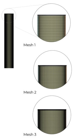
Figure 4.
Numerical grids subjected to grid independence study.
In the next step, the numerical grids were compared in terms of the results obtained. The dependence of the mean temperature of the condenser walls (Figure 5) and the adiabatic section (Figure 6) with respect to time and the value of thermal resistance of the thermosyphon (Table 5) were considered. All cases were calculated for the evaporation–condensation phase transition model.
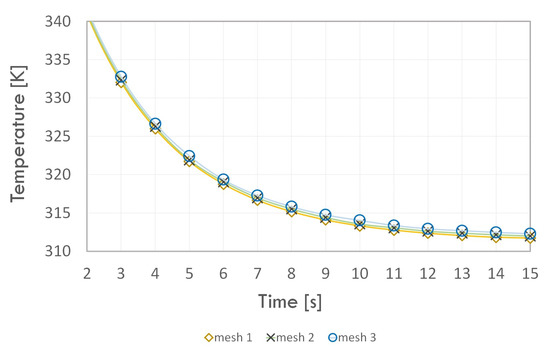
Figure 5.
Average condenser wall temperature versus time.
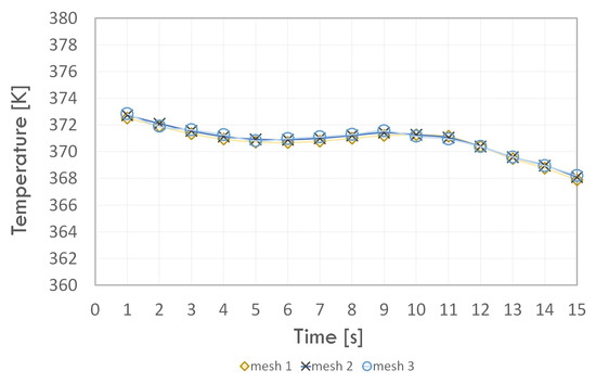
Figure 6.
Average adiabatic section wall temperature vs. time.
Table 5.
Thermal resistance value for each grid.
By analysing the wall temperature dependence of each section for the three numerical grids, we concluded that the introduction of higher density mesh elements in the fluid and solid domain area did not have much effect on the temperature value. Moreover, the value of the thermal resistance error for Grid 1 compared to Grid 3 did not exceed 1%; hence, Grid 1 was used in further study. The minimum orthogonal quality value of the selected grid was equal to 0.60, which means that it can be successfully used in the next stage of analysis.
3. Calculation Results and Analysis
The results in the form of temperature distribution along the thermosyphon at the 15th second of the simulation are shown in Figure 7. The temperature measurement points on the walls were selected based on the position of the thermocouples used in the study [9]. The CFD calculations based on the Lee model included in the four cases carried out for this paper were compared with experimental measurements and CFD calculations by Fadhl [9] and Kim [37].
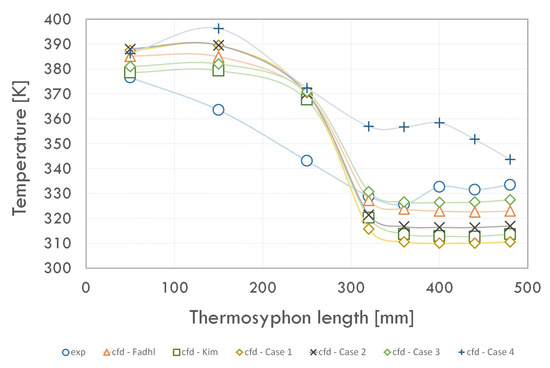
Figure 7.
Temperature distribution on thermosyphon walls.
We concluded that the results of all the CFD analysis performed deviate (at some measurement points) from the experimental results. However, using the source terms described in the UDF file used (Case 2–3) allowed for a better prediction of the temperature distribution along the thermosyphon compared to the evaporation–condensation model. The results obtained with this solution had a lower error than those obtained using the Lee model. The adoption of a variable value of the mass transfer time relaxation parameter during condensation (r) for Case 2 and Case 3 enabled a more accurate prediction of temperature in the condenser and evaporator. However, assuming the value of the parameter r = 10 (Case 4) led to an overestimation of the temperatures along the entire thermosyphon.
For the phenomenon studied under the given conditions, the value of this coefficient is r = 1 (Case 3). Assuming the value of mass transfer time relaxation parameter during evaporation equal to r = 0.1 (Case 2) resulted in more apparent underestimation of condenser temperatures and overestimation of evaporator temperatures relative to experimental studies. By comparing the results of the CFD analysis performed by Fadhl [9] and Kim [37], the model described by Case 3 can predict the evaporator temperature to a similar extent and, at the same time, allows for a more accurate determination of the condenser wall temperature.
Figure 8, Figure 9 and Figure 10 show the average wall temperature values for each section during the simulation run. For the evaporator section (Figure 8), the temperature value of the wall for all cases in the first second of the simulation did not differ much and was in the range of 378–380 K. This was due to the assumption that the same initial condition was in the form of the initial temperature of 373.15 K. Then, an increase in the wall temperature was observed. However, this value increased the fastest for Cases 1 and 4. A slightly slower increase in temperature in the evaporator section occurred for Case 2.
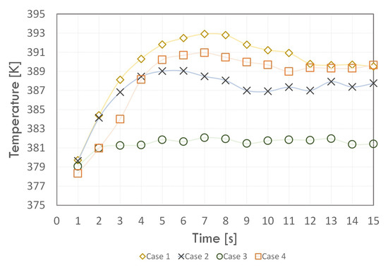
Figure 8.
The time dependence of the average evaporator wall temperature.
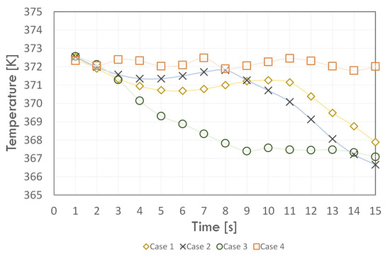
Figure 9.
The mean temperature trend of the adiabatic zone.
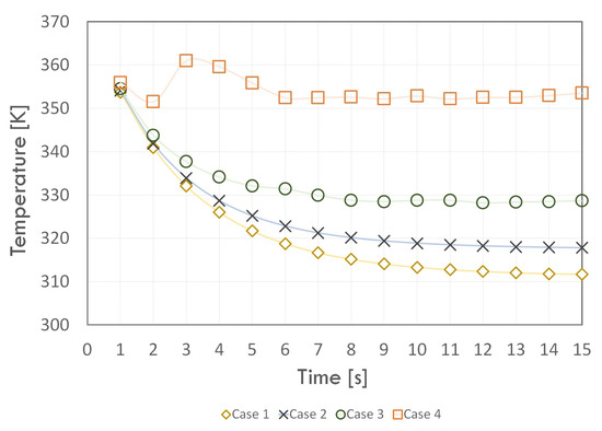
Figure 10.
The condenser wall temperature change.
However, for Case 3, the temperature of the evaporator walls increased only to 2 s of simulation and then stabilised within 382 K. For Cases 1, 2, and 4, the temperature value reached its maximum value, then it slowly decreased, and, for about 12 s of the analysis, it stabilised. The average evaporator wall temperature was stabilised due to steady heat flux. The temperature value in the last time step (15 s) for Cases 1 and 4 was almost 390 K, while for Case 2, it was almost 388 K.
The wall temperature of the adiabatic section (Figure 9) for each case had variable values during the simulation; however, the final value for Cases 1, 2, and 3 were very similar. At the beginning of the simulation, the average wall temperature of the adiabatic section was practically the same for all cases due to the initial condition. For Case 4, during the whole simulation time, it varied between 372 and 373 K. However, for the other cases, the temperature decreased at the beginning of the simulation: for Case 2 to a value of about 371.5 K, for Case 1 to a value below 370.5 K, and for Case 3 to a value of about 367.5 K. For Case 3, the temperature value stabilised from the 9 s of the simulation and was 376.5 K. For Case 2, a decrease in the temperature value was observed from the 8 s of analysis to a value of almost 366.5 K in the last time step.
On the other hand, for Case 1, the value of the average temperature of the adiabatic section walls decreased from the 11 s of the simulation, reaching a final value of 368 K. On the other hand, for the condenser walls (Figure 10), the temperature for all cases decreases and stabilises in successive time steps. As for the other sections, in the initial time steps, the value of the condenser wall temperature had a similar value. In contrast to the other cases, for Case 4, the temperature initially decreased, then in a time of 3 s, it reached a maximum value of more than 360 K. Then, it decreased, and, after 6 s, it reached a constant value of about 353 K. For the other cases, the temperature initially decreased.
The condenser wall temperature reached a constant value around 312, 318, and 329 K for times of 12, 8, and 12 s and Cases 1, 2, and 3, respectively. Hence, the previous conclusions regarding the negative effect of taking too high a r value, i.e., r, on the phase change phenomenon remain valid. Taking the value of r = 1, with a variable value of r, led to temperature values close to the experimental data. However, the value of r < 1, especially for the condenser section, caused an overestimation of the average value of the wall temperature at each time step. The average temperature was stabilized the fastest for Case 3 and each section.
Table 6 shows the thermal resistance value calculated from the experiment and individual CFD studies. The thermal resistance R of the tested thermosyphon was calculated from Equation (26) [9]. Its value depends on the heat flux delivered to the evaporator and on the values of the mean wall temperatures of the evaporator T and condenser T.
Table 6.
Thermal resistance values.
Figure 11 shows the variation of thermal resistance values over time for the simulations performed in this work and summarises the relative percentage error for the experimentally determined value. At the simulation beginning, a similar thermal resistance was observed for each case (below 0.07 K/W) and then the value increased. For Case 4, the thermal resistance had a different trend from the other cases—up to the 2 s of the analysis, there was an increase, then a decrease, and then an increase again. The thermal resistance value stabilised in 6 s of simulation, and its value was almost 0.1 K/W. For Cases 1–3, the thermal resistance value increased and then stabilised from the 8 s of simulation. The final values of thermal resistance were almost 0.21, 0.19, and 0.14 K/W for Cases 1, 2, and 3, respectively.
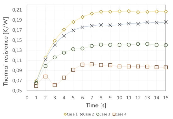
Figure 11.
Thermal resistance values versus simulation time.
We concluded that the multiphase model introduced using the UDF script in Case 3 best reflected the temperature values in all sections of the thermosyphon. It also provided a much smaller value of thermal resistance error compared to the other cases as well as the studies done by Kim [37], and Fadhl [9]. Although the phase change model proposed in Case 4 introduced the smallest thermal resistance error, it dramatically overestimated the condenser temperatures, and thus this result appears to be unreliable. Figure 12 shows the distribution of the volume fraction of the liquid phase at given time points. It is possible to observe with them the boiling phenomenon where heat is removed from the evaporator section.
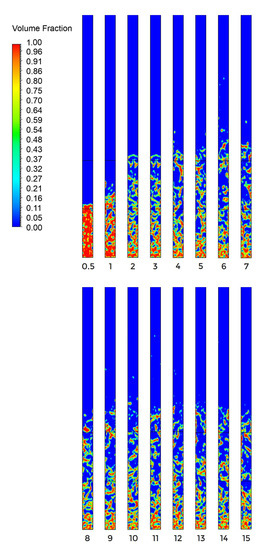
Figure 12.
Distribution of the liquid fraction at selected time steps (Case 3).
A blue colour illustrates only liquid, whereas a red colour stands for the presence of only vapour. The liquid initially filled 50% of the evaporator, which was heated by applying a constant heat flux to the evaporator section’s wall. Subsequently, heat was conducted through the walls of the thermosyphon, and, in the areas where the liquid reached the value of the saturation temperature, a phase change occurred. As a result, nucleation sites began to form, and subsequently vapour bubbles were formed. The bubbles were transported upwards, where they broke up, and consequently an increase in the vapour volume fraction was observed. After two seconds (Case 3), the vapour volume fraction did not change rapidly due to steady-state heat transfer.
As a result of the study, we decided to compare the value of the heat transfer coefficient in the evaporator section. This value for the condenser walls was determined by applying a boundary condition. The value of the heat transfer coefficient in the evaporator walls was calculated based on experimental investigations, relevant correlations, and numerical studies carried out by the authors (Cases 1–4), and simulations performed by Fadhl [9] and Kim [37] are presented in Table 7.
Table 7.
Heat transfer coefficients.
Regarding Labuntsov’s correlation (Equation (27)), the value of the heat transfer coefficient in the evaporator can be written by the formula [51]:
The correlation produced by Kruzhilin (Equation (28)) to obtain the heat transfer coefficient in the evaporator section is [52]:
The value of can be determined using Equation (29) as described in Robinson’s study [53] based on the heat flux density applied to the evaporator q, the evaporator wall temperature as well as the saturation temperature :
Equation (29) was used to determine for both the experimental and CFD study carried out by the authors of the article as well as Fadhl and Kim. The temperature for all cases was taken as the value of the wall temperature at half the height of the initial evaporator filling with the working medium (50 mm from the bottom base of the thermosyphon).
Then the comparison of the values of , determined from experimental and numerical studies, proceeded. We concluded that, although the difference in the values of was significant, the uncertainty of the temperature measurement during the experiment [9] introduced an uncertainty of the coefficient equal to about ±1000 W/m2K. This shows that the value of the heat transfer coefficient was sensitive to even small temperature changes. The application of the = 1 and the variable value of the (Case 3) in comparison with the other cases (Cases 1, 2, and 4) allowed us to obtain the lowest error (referring to the experimental studies).
The fact that Kim’s numerical study resulted in a more accurate value of indicates a lower error during the measurement of the evaporator temperature. However, the model developed by Kim reproduced the temperature values in the condenser with less accuracy. Although the experimental results differ from the results obtained using correlations [51,52], numerous studies show that correlations are sensitive to the value of the fill factor [54,55,56]. In addition, the results of calculations using other correlations can vary significantly, as described in the thesis [9].
4. Summary and Conclusions
In this paper, the phenomenon of phase change of the medium in the thermosyphon was numerically simulated. For the CFD analysis, a UDF script was created to allow additional source equations to be entered. This script was used in the study of a two-dimensional thermosyphon model, thus, considering four cases of calculations depending on the values of the assumed r and r coefficients.
- By comparing the results obtained in the different cases, we observed that, by taking the value of coefficient r = 1 and the variable value of coefficient r that depended on the density of the two phases, we obtained the results of the temperature distribution in the thermosyphon that were the most similar to those obtained experimentally.
- Concerning the results obtained by Kim [37] and Fadhl [9], the value of coefficient r, as well as the variable value of coefficient r, are of great importance in the numerical study of the phase change phenomenon of the medium. Assuming a value of r = 1 allowed for similar temperature distribution in the evaporator as in other numerical studies [9,37]. At the same time, the condenser conditions were determined with greater accuracy (for experimental studies), resulting in a more precise determination of thermal resistance values.
- As a result of the simulations, we found that taking the value of r = 10 for Case 4 led to an overestimation of temperatures along the entire thermosyphon. Hence, for the phenomenon of the phase change of the medium in the thermosyphon (for the conditions specified above), the corresponding value of the mass transfer time relaxation coefficient during evaporation was r = 1.
- The conducted studies show the need for further modification of the Volume of Fluid multiphase model. It was indicated that, for a particular case, an appropriate adaptation of both the mass transfer time relaxation parameter during evaporation and condensation played an important role.
- The tests carried out in the two-dimensional case made it possible to observe the phenomenon of evaporation of the working medium in the thermosyphon. Based on the volume fraction distribution of the liquid phase, we concluded that the Volume of Fluid model was able to predict the formation of the boundary between the two phases well.
Thus, to properly analyse the phenomenon of heat extraction by the thermosyphon, additional experiments would have to be conducted under strictly defined operating conditions. More temperature measurements of the evaporator section would also need to be provided, as this section appears to have a more uneven distribution, especially for low fill ratios. As a further direction of this research, the authors propose to research the impact of the operating parameters in the context of liquid entrainment or sonic limitation.
Author Contributions
Conceptualization, G.C.; Investigation, G.C.; Methodology, G.C. and J.W.; Supervision, J.W.; Validation, G.C.; Writing—original draft, G.C. and J.W. Both authors have read and agreed to the published version of the manuscript.
Funding
This research received no external funding.
Institutional Review Board Statement
Not applicable.
Informed Consent Statement
Not applicable.
Data Availability Statement
Data sharing not applicable.
Acknowledgments
This research was supported by national subvention no. 16.16.130.942.
Conflicts of Interest
The authors declare no conflict of interest.
Abbreviations
The following abbreviations are used in this manuscript:
| volume fraction of the liquid phase [-], | |
| volume fraction of the vapor phase [-], | |
| density of the liquid phase [kg/m], | |
| density of the vapor phase [kg/m], | |
| density [kg/m], | |
| p | pressure [Pa], |
| t | time [s], |
| T | temperature of the liquid phase [K], |
| T | saturation temperature [K], |
| T | temperature of the saturated vapor [K], |
| H | vaporization enthalpy [J/kg], |
| h | heat transfer coefficient [W/(m2K)], |
| L | characteristic linear dimension [m], |
| thermal conductivity [W/(m·K)], | |
| M | molecular weight [kg/kmol], |
| S | source term in the mass conservation equation [kg/m3s], |
| S | source term in the energy equation [J/m3s], |
| r | mass transfer time relaxation parameter during evaporation [1/s], |
| r | mass transfer time relaxation parameter during condensation [1/s], |
| D | mean Sauter diameter [m], |
| R | universal gas constant [J/(mol·K)], |
| x, y, z | Cartesian coordinates [m], |
| T | temperature [K], |
| c | specific heat of the material [J/(kg·K)], |
| density of the material [kg/m], | |
| thermal conductivity of the material [W/(m·K)], | |
| q | heat generation inside material [W/m], |
| F | Continuum Surface Force [N], |
| surface tension of liquid-vapor interface during evaporation [N/m], | |
| g | gravitational acceleration [N/kg], |
| dynamic viscosity [kg/(m·s)], | |
| I | unit tensor [1/s], |
| specific heat of the liquid phase [J/(kg·K)], | |
| specific heat of the vapor phase [J/(kg·K)], | |
| internal energy of the liquid phase [J/kg], | |
| internal energy of the vapor phase [J/kg], | |
| e | internal energy [J/kg], |
| h | heat transfer coefficient in the evaporator [W/(m2K)], |
| thermal conductivity of the liquid phase [W/(m · K)], | |
| kinematic viscosity [m/s], | |
| q | heat flux density applied to the evaporator [W/m], |
| Pr | Prandtl number of the liquid phase [-]. |
References
- Cotter, T.P. Theory of Heat Pipes, 1st ed.; Los Alamos Scientific Laboratory of the University of California: Los Alamos, NM, USA, 1965; pp. 7–8. [Google Scholar]
- Jaworski, M. Techniki chłodzenia elementów elektronicznych. Artykuł przeglądowy. Chłodnictwo 2007, 12, 32–39. [Google Scholar]
- Galvis, E.; Culham, R. Measurements and flow pattern visualizations of two-phase flow boiling in single channel microevaporators. Int. J. Multiph. Flow 2012, 42, 52–61. [Google Scholar] [CrossRef]
- Faghri, A. Review and advances in heat pipe science and technology. J. Heat Transf. 2012, 134, 123001. [Google Scholar] [CrossRef]
- Peterson, G.P. An Introduction to Heat Pipes: Modeling, Testing, and Applications, 1st ed.; John Wiley & Sons: New York, NY, USA, 1994; pp. 1–15, 230–270. [Google Scholar]
- Wójcik, J. Chłodzenie Procesorów PC, 1st ed.; Helion: Gliwice, Poland, 2020; pp. 19–38. [Google Scholar]
- Zhang, H.; Shao, S.; Tian, C.; Zhang, K. A review on thermosyphon and its integrated system with vapor compression for free cooling of data centers. Renew. Sustain. Energy Rev. 2018, 81, 789–798. [Google Scholar] [CrossRef]
- Chen, J.-S.; Chou, J.-H. The length and bending angle effects on the cooling performance of flat plate heat pipes. Int. J. Heat Mass Transf. 2015, 90, 848–856. [Google Scholar] [CrossRef]
- Fadhl, B. Modelling of the Thermal Behaviour of a Two-Phase Closed Thermosyphon. Ph.D. Thesis, Department of Mechanical, Aerospace and Civil Engineering College of Engineering, Design and Physical Sciences, Brunel University, London, UK, 2015. [Google Scholar]
- Li, Z.; Sarafraz, M.M.; Mazinani, A.; Moria, H.; Tlili, I.; Alkanhal, T.A.; Goodarzi, M.; Safaei, M.R. Operation analysis, response and performance evaluation of a pulsating heat pipe for low temperature heat recovery. Energy Convers. Manag. 2020, 222, 113230. [Google Scholar] [CrossRef]
- Sarafraz, M.M.; Tian, Z.; Tlili, I.; Kazi, S.; Goodarzi, M. Thermal evaluation of a heat pipe working with n-pentane-acetone and n-pentane-methanol binary mixtures. J. Therm. Anal. Calorim. 2019, 139, 2435–2445. [Google Scholar] [CrossRef]
- Li, Z.; Sarafraz, M.M.; Mazinani, A.; Hayat, T.; Alsulami, H.; Goodarzi, M. Pool boiling heat transfer to CuO-H2O nanofluid on finned surfaces. Int. J. Heat Mass Transf. 2020, 156, 119780. [Google Scholar] [CrossRef]
- Peng, Y.; Khaled, U.; Al-Rashed, A.A.; Meer, R.; Goodarzi, M.; Sarafraz, M.M. Potential application of Response Surface Methodology (RSM) for the prediction and optimization of thermal conductivity of aqueous CuO (II) nanofluid: A statistical approach and experimental validation. Phys. A Stat. Mech. Appl. 2020, 554, 124353. [Google Scholar] [CrossRef]
- Goshayeshi, H.R.; Goodarzi, M.; Dahari, M. Effect of magnetic field on the heat transfer rate of kerosene/Fe2O3 nanofluid in a copper oscillating heat pipe. Exp. Therm. Fluid Sci. 2015, 68, 663–668. [Google Scholar] [CrossRef]
- Başaran, T.; Küçüka, S. Flow through a rectangular thermosyphon at specified wall temperatures. Int. Commun. Heat Mass Transf. 2003, 30, 1027–1039. [Google Scholar] [CrossRef]
- Liu, S.; Li, J.; Chen, Q. Visualization of flow pattern in thermosyphon by ECT. Flow Meas. Instrum. 2007, 18, 216–222. [Google Scholar] [CrossRef]
- Legierski, J.; Wie, B.; De Mey, G. Measurements and simulations of transient characteristics of heat pipes. Microelectron. Reliab. 2006, 46, 109–115. [Google Scholar] [CrossRef]
- Ramalingam, V.; Annamalai, A.S. Experimental investigation and computational fluid dynamics analysis of a air cooled condenser heat pipe. Therm. Sci. 2011, 15, 759–772. [Google Scholar]
- Lee, W.H. Pressure iteration scheme for two-phase flow modeling. In Multiphase transport: Fundamentals, Reactor Safety, Applications; Hemisphere Publishing: Washington, DC, USA, 1980; pp. 407–432. [Google Scholar]
- De Schepper, S.C.; Heynderickx, G.J.; Marin, G.B. Modeling the evaporation of a hydrocarbon feedstock in the convection section of a steam cracker. Comput. Chem. Eng. 2009, 33, 112–132. [Google Scholar] [CrossRef]
- ANSYS FLUENT 12.0 User’s Guide. Available online: https://www.afs.enea.it/project/neptunius/docs/fluent/html/th/node344.htm (accessed on 20 December 2020).
- Wu, H.L.; Peng, X.F.; Ye, P.; Gong, Y.E. Simulation of refrigerant flow boiling in serpentine tubes. Int. J. Heat Mass Transf. 2007, 50, 1186–1195. [Google Scholar] [CrossRef]
- De Schepper, S.C.; Heynderickx, G.J.; Marin, G.B. CFD modeling of all gas–liquid and vapor–liquid flow regimes predicted by the Baker chart. Chem. Eng. J. 2008, 138, 349–357. [Google Scholar] [CrossRef]
- Alizadehdakhel, A.; Rahimi, M.; Alsairafi, A.A. CFD modeling of flow and heat transfer in a thermosyphon. Int. Commun. Heat Mass Transf. 2010, 37, 312–318. [Google Scholar] [CrossRef]
- Lin, Z.; Wang, S.; Shirakashi, R.; Zhang, L.W. Simulation of a miniature oscillating heat pipe in bottom heating mode using CFD with unsteady modeling. Int. J. Heat Mass Transf. 2013, 57, 642–656. [Google Scholar] [CrossRef]
- Fadhl, B.; Wrobel, L.C.; Jouhara, H. Numerical modelling of the temperature distribution in a two-phase closed thermosyphon. Appl. Therm. Eng. 2013, 60, 122–131. [Google Scholar] [CrossRef]
- Fadhl, B.; Wrobel, L.C.; Jouhara, H. CFD modelling of a two-phase closed thermosyphon charged with R134a and R404a. Appl. Therm. Eng. 2015, 78, 483–490. [Google Scholar] [CrossRef]
- Zhao, Z.; Zhang, Y.; Zhang, Y.; Zhou, Y.; Hu, H. Numerical Study on the Transient Thermal Performance of a Two-Phase Closed Thermosyphon. Energies 2018, 11, 1433. [Google Scholar] [CrossRef]
- Yang, Z.; Peng, X.F.; Ye, P. Numerical and experimental investigation of two phase flow during boiling in a coiled tube. Int. J. Heat Mass Transf. 2008, 51, 1003–1016. [Google Scholar] [CrossRef]
- Fang, C.; David, M.; Rogacs, A.; Goodson, K. Volume of Fluid Simulation of Boiling Two-Phase Flow in a Vapor-Venting Microchannel. Front. Heat Mass Transf. 2010, 1. [Google Scholar] [CrossRef]
- Tonini, S.; Cossali, G. Moving boundary and time-dependent effects on mass transfer from a spherical droplet evaporating in gaseous environment. In Proceedings of the ICMF-2016—9th International Conference on Multiphase Flow, Firenze, Italy, 22–27 May 2016. [Google Scholar]
- Das, K.; Manepally, C.; Fedors, R.; Basu, D. Numerical and Experimental Study of In-Drift Heat and Mass Transfer Processes; Center for Nuclear Waste Regulatory Analyses: San Antonio, TX, USA, 2011. [Google Scholar]
- Xu, Z.; Zhang, Y.; Li, B.; Huang, J. Modeling the phase change process for a two-phase closed thermosyphon by considering transient mass transfer time relaxation parameter. Int. J. Heat Mass Transf. 2016, 101, 614–619. [Google Scholar] [CrossRef]
- Kafeel, K.; Turan, A. Axi-symmetric simulation of a two phase vertical thermosyphon using Eulerian two-fluid methodology. Heat Mass Transf. 2013, 49, 1089–1099. [Google Scholar] [CrossRef]
- Kafeel, K.; Turan, A. Simulation of the response of a thermosyphon under pulsed heat input conditions. Int. J. Therm. Sci. 2014, 80, 33–40. [Google Scholar] [CrossRef]
- Wang, H. Analytical and Computational Modeling of Multiphase Flow in Ferrofluid Charged Oscillating Heat Pipes. Doctor Dissertation, The Graduate Faculty in Partial Fulfillment of the Requirements for the Degree of Doctor of Philosophy Mechanical Engineering, University Of Oklahoma, Norman, OK, USA, 2020. [Google Scholar]
- Kim, Y.; Choi, J.; Kim, S. Effects of mass transfer time relaxation parameters on condensation in a thermosyphon. J. Mech. Sci. Technol. 2015, 29, 5487–5505. [Google Scholar] [CrossRef]
- Chu, W.-X.; Shen, Y.-W.; Wang, C.-C. Enhancement on heat transfer of a passive heat sink with closed thermosyphon loop. Appl. Therm. Eng. 2021, 183, 116243. [Google Scholar] [CrossRef]
- Huang, C.-N.; Lee, K.-L.; Tarau, C.; Kamotani, Y.; Kharangate, C.R. Computational fluid dynamics model for a variable conductance thermosyphon. Case Stud. Therm. Eng. 2021, 25, 100960. [Google Scholar] [CrossRef]
- Wang, W.-W.; Cai, Y.; Wang, L.; Liu, C.-W.; Zhao, F.-Y.; Sheremet, M.-A.; Liu, D. A two-phase closed thermosyphon operated with nanofluids for solar energy collectors: Thermodynamic modeling and entropy generation analysis. Sol. Energy 2020, 211, 192–209. [Google Scholar] [CrossRef]
- Nguyen, T.; Merzari, E. Computational fluid dynamics simulation of a single-phase rectangular thermosyphon. In Proceedings of the 2020 International Conference on Nuclear Engineering Collocated with the ASME 2020 Power Conference, American Society of Mechanical Engineers Digital Collection, Virtual, Anaheim, CA, USA, 4–5 August 2020; Volume 3. [Google Scholar]
- Cisterna, L.H.; Fronza, E.L.; Cardoso, M.C.; Milanez, F.H.; Mantelli, M.B. Modified Biot Number Models For Startup And Continuum Limits Of High Temperature Thermosyphons. Int. J. Heat Mass Transf. 2021, 165, 120699. [Google Scholar] [CrossRef]
- Ng, V.O.; Yu, H.; Wu, H.A.; Hung, Y.M. Thermal performance enhancement and optimization of two-phase closed thermosyphon with graphene-nanoplatelets coatings. Energy Convers. Manag. 2021, 236, 114039. [Google Scholar] [CrossRef]
- Wołoszyn, J.; Gołaś, A. Experimental verification and programming development of a new MDF borehole heat exchanger numerical model. Geothermics 2016, 59, 67–76. [Google Scholar] [CrossRef]
- Kamburova, V.; Ahmedov, A.; Iliev, I.K.; Beloev, I.; Pavlović, I.R. Numerical Modelling of the Operation Of A Two-Phase Thermosyphon. Therm. Sci. 2018, 22, 1311–1321. [Google Scholar] [CrossRef]
- Wołoszyn, J. Influence of Material, Design and Operating Parameters on the Underground Thermal Energy Storage Efficiency; AGH University of Science and Technology Press: Krakow, Poland, 2019. [Google Scholar]
- Tarokh, A.; Bliss, C.; Hemmati, A. Performance enhancement of a two-phase closed thermosyphon with a vortex generator. Appl. Therm. Eng. 2021, 182, 116092. [Google Scholar] [CrossRef]
- Wang, X.; Yao, H.; Li, J.; Wang, Y.; Zhu, Y. Experimental and numerical investigation on heat transfer characteristics of ammonia thermosyhpons at shallow geothermal temperature. Int. J. Heat Mass Transf. 2019, 182, 116092. [Google Scholar] [CrossRef]
- Brackbill, J.U. A continuum method for modeling surface tension. J. Comput. Phys. 1992, 100, 336–354. [Google Scholar] [CrossRef]
- Wang, X.; Liu, H.; Wang, Y.; Zhu, Y. CFD simulation of dynamic heat transfer behaviors in super-long thermosyphons for shallow geothermal application. Appl. Therm. Eng. 2020, 174, 115295. [Google Scholar] [CrossRef]
- Labuntsov, D.A. Heat transfer problems with nucleate boiling of liquids. Therm. Eng. 1972, 19, 21–22. [Google Scholar]
- Kruzhilin, G.N. Free-convection transfer of heat from a horizontal plate and boiling liquid. Dokl. AN SSSR (Rep. USSR Acad. Sci.) 1947, 58, 1657–1660. [Google Scholar]
- Robinson, A.J.; Smith, K.; Hughes, T.; Filippeschi, S. Heat and mass transfer for a small diameter thermosyphon with low fill ratio. Int. J. Thermofluids 2020, 1–2, 100010. [Google Scholar] [CrossRef]
- Ahmad, H.H. Heat Transfer Characteristics in a Heat Pipe Using Water-Hydrocarbon Mixture as a Working Fluid. (An Experimental Study). Al-Rafidain Eng. 2012, 20, 128–137. [Google Scholar]
- Sadrameli, S.M.; Forootan, D.; Farajimoghaddam, F. Effect of working fluid inventory and heat input on transient and steady state behavior of a thermosyphon. J. Therm. Anal. Calorim. 2021, 143, 3825–3834. [Google Scholar] [CrossRef]
- Noie, S.H. Heat transfer characteristics of a two-phase closed thermosyphon. Appl. Therm. Eng. 2005, 25, 495–506. [Google Scholar] [CrossRef]
Publisher’s Note: MDPI stays neutral with regard to jurisdictional claims in published maps and institutional affiliations. |
© 2021 by the authors. Licensee MDPI, Basel, Switzerland. This article is an open access article distributed under the terms and conditions of the Creative Commons Attribution (CC BY) license (https://creativecommons.org/licenses/by/4.0/).