
Offshore Wind Potential of West Central Taiwan: A Case Study

Department of Biomechatronics Engineering, National Taiwan University, No. 1, Sec. 4, Roosevelt Road, Taipei 10617, Taiwan
*
Author to whom correspondence should be addressed.
Energies 2021, 14(12), 3702; https://doi.org/10.3390/en14123702
Submission received: 19 April 2021
/
Revised: 9 June 2021
/
Accepted: 17 June 2021
/
Published: 21 June 2021
(This article belongs to the Topic Exergy Analysis and Its Applications)
Abstract
:In this study, we present the wind distributions from a long-term offshore met mast and a novel approach based on the measure–correlate–predict (MCP) method from short-term onshore-wind-turbine data. The annual energy production (AEP) and capacity factors (CFs) of one onshore and four offshore wind-turbine generators (WTG) available on the market are evaluated on the basis of wind-distribution analysis from both the real met mast and the MCP method. Here, we also consider the power loss from a 4-month light detection and ranging (LiDAR) power-curve test on an onshore turbine to enhance the accuracy of further AEP and CF evaluations. The achieved Weibull distributions could efficiently represent the probability distribution of wind-speed variation, mean wind speed (MWS), and both the scale and shape parameters of Weibull distribution in Taiwan sites. The power-loss effect is also considered when calculating the AEPs and CFs of different WTGs. Successful offshore wind development requires (1) quick, accurate, and economical harnessing of a wind resource and (2) selection of the most suitable and efficient turbine for a specific offshore site.
1. Introduction
The global necessity of developing renewable energy is rising due to climate change and the exhaustion of fossil-fuel-based energy sources. According to an Intergovernmental Panel on Climate Change (IPCC) report, renewable-energy sources have the potential to reduce carbon emissions and solve the climate crisis [1]. As a result, renewable energy could play a key role in the post-oil era by providing stable and clean energy [2]. Wind-power energy was developed in the 1990s in Europe, and Denmark installed the first offshore wind farm (OWF) in 1991 [3]. Many countries have since launched related programs for offshore-wind-power (OWP) development. Wind energy is the fastest growing renewable-energy source, receiving global attention due to advances in technology for harnessing its power. The utilization of wind power is an answer to environmental and climate-change problems and is a means of conserving conventional-energy sources. To catalyze the development of wind farms, several global research projects are being run to assess wind potential and predict wind energy [4].
Compared to onshore wind energy, offshore wind energy provides more stable output and higher energy density, has smaller scale restrictions, and is less likely to cause civil complaints [5]. Consequently, offshore wind power has been the official energy policy in Europe for many years. The ratio of renewable energy reached 20% of total power usage on the basis of the EU program in 2020, in which offshore wind energy plays a crucial role. The Global Wind Energy Council (GWEC) in 2018 estimated the annual installed capacity of global offshore wind power to 2017 as 18,814 MW in 17 countries, with 11 in Europe accounting for 15,780 MW, equivalent to 84% of total capacity, and the other 16% for Taiwan, Vietnam, the US, South Korea, etc. [6]. The installed capacities in the top two countries, the UK and Germany, were 6836 and 5355 MW, equivalent to 36% and 28.5%, respectively [7]. China had the third largest installed capacity at 2788 MW, accounting for 15%, followed by Denmark. There are still more undeveloped offshore wind farms in Taiwan.
In Taiwan, over 98% of the energy supply is imported from other countries, particularly fossil fuels (81.5%) [8]. Therefore, the Taiwanese government is actively developing renewable energy, especially in the offshore wind sector. The goal of installed capacity of offshore wind power in Taiwan was 520 MW in 2020 and will reach 5500 MW in 2025. Offshore wind power has three planning stages, namely, demonstration wind farm, potential wind-farm development, and zone development. The stakeholders who joined the first stage (demonstration wind farm) are Taipower, SWancor, and TGC. These stakeholders individually completed the installation of offshore met masts in March 2015 and have since measured long-term offshore wind data. SWancor finished the first two offshore wind turbines near the Miauli coast and achieved an 8 MW installation capacity in October 2016, which extended the frontier of the offshore-wind-power industry in Taiwan. The development of offshore wind farms in Taiwan has passed the planning stage and is moving to extensively set up wind turbines. Phenomena such as frequent typhoons and earthquakes have made Taiwan a leader in offshore-wind-power development in Asia by finding a tremendous and essentially infinite energy source in Earth’s seas.
The most promising marine energy sources are offshore wind energy and wave energy [9]. Wave-energy harvesting is still in the early stages of development; therefore, a potential solution for the acceleration of its development is the combination of two different energy resources [10]. Wind power plays a key role in reducing global carbon emissions. The power curve provided by wind-turbine manufacturers offers an effective way of presenting the global performance of wind turbines; however, due to the complicated dynamic nature of offshore wind turbines and the harsh environment in which they are operating, wind-power forecasting is challenging, but it is vital to enable condition monitoring (CM) [11]. The future of offshore energy harvesting relies upon further technological advancements of wind-turbine generators (WTG), national policies, and the number of large companies and developers involved in this sector. A key issue regarding the development of offshore wind harvesting is wind distribution and machine selection. Therefore, huge amounts of offshore wind energy could be developed in Taiwan in three decades; however, generating this offshore-wind-energy supply in Taiwan requires an accurately and economically represented wind distribution, the prediction of wind-farm output, and the selection of suitable machines.
In this study, we propose an applicable wind-power estimation of Taiwan offshore sites via a long-term operating met mast and demonstrate a prediction method for wind resources from short-term near-shore data. Lastly, the AEPs or CFs of several market-available turbine types are explored to identify the most efficient machine in offshore sites, and the gap between met-mast and prediction-method data.
2. Theories of Wind Energy Systems
2.1. Wind
Wind is the large-scale air flow on Earth’s surface. Winds are commonly classified by their spatial scale, their speed, the types of forces that cause them, the regions in which they occur, and their effect. Some wind characteristics are velocity (wind speed), density, content, and energy. In this section, we introduce the basic definitions of wind and related theorems of wind-energy assessment.
- A.
- Wind EnergyWind power is the application of wind to provide mechanical power through wind turbines for generating electrical power. The kinetic energy in a parcel of air of mass m flowing at speed v in the x direction is given by Equation (1):where Λ denotes the cross-sectional area in m2, ρ is air density in kg/m3, and x denotes the thickness of the parcel in m.
- B.
- Wind PowerWind power passing through an area Λ perpendicular to the wind is given by the following:This can be viewed as the power being supplied at the origin to cause the energy of the parcel to increase according to Equation (1). A wind turbine extracts power from side x, with Equation (2) representing the total power available at this surface for possible extraction. The wind industry needs to be able to describe variations in wind speed. Turbine designers need this information to optimize their designs, thus minimizing generating costs. Wind-farm developers also need wind distribution to predict the AEP and to select a turbine to maximize the power production. Wind variation for a typical site is usually described using the so-called Weibull distribution, as shown in Figure 1 and Figure 2. Figure 1 shows the curves of Scale Factor 1 with different shape factors. Figure 2 shows the curves of Shape Factor 3 with different scale factors.
- C.
- Weibull Distribution
- D.
- Mean Wind SpeedThis is a two-parameter distribution, where A and k denote the scale and shape parameters, respectively. Wind speed v is distributed as Weibull distribution f(v). Mean wind speed is derived as [16]:If the change in variable is as follows,then the mean wind speed can be expressed asGamma function (y) is generally written in the following form:
- E.
- Wind-Speed VarianceEquations (6) and (7) have the same integral if y = 1 + 1/k. Mean wind speed and variance are thenScale parameter A and shape parameter k can then be derived from the average wind speed and variance on the basis of Weibull distribution. On the basis of this equation, the ratio of common wind speed rises with rising k. Acquired data at many widely spread locations can be naturally well-defined by Weibull density function over a long-enough time period.Scale parameter A can scale the curves to fit different wind-speed distributions, as shown by Equation (3). Since the properties of a probability density function entail that the area under the curve must be unity, then the curve has to horizontally expand as it is vertically compressed. Therefore, corresponding wind-speed distribution may be adopted for any value of A with the appropriate scale parameter.
- F.
- Measure–Correlate–Predict MethodIf no or a few measurements are available for estimating the wind-energy resource at a given potential windfarm site, then available measurements should be supplemented by measurements over a longer period from another site. This method is based on the assumption that the overall wind climate remains the same within a distance given by local mesoscale conditions [17].Renewable-energy researchers have applied measure–correlate–predict (MCP) algorithms for many years to construct wind-resource models with the long-term conditions at a specific site based on short-term wind-data collection. MCP algorithms are used to predict a wind resource by modeling wind data (speed and direction) measured at the special site over up to a year, together with coexisting data at a neighboring reference site. The model employs long-term data from the site to simulate and analyze the long-term wind distributions at the target site. In general, MCP characterizes wind-speed distributions as a function of wind direction at a target site to obtain the annual energy estimation of a wind farm located there. Local obstruction, atmosphere gradient, large-scale weather influence, and terrain effects induce stochastic variations of wind speed and direction for spread of distance and time. Therefore, corresponding models and coexisting wind data should be considered carefully to improve the consistency between simulation and actual results. Well over half a dozen variations on the MCP technique have been proposed over the last 15 years, in part to address some of the specific concerns mentioned above [18]. The variations include two-dimensional, vector, and nonlinear-regression techniques [19], matrix approaches [20], artificial neural networks [21,22,23], and joint probability distributions [24,25,26].MCP methods fundamentally differ in the relationships that they establish between wind data (speed and direction) recorded at the target site and simultaneously recorded wind data at one or various nearby weather stations that serve as reference stations and for which long-term data series are available.
2.2. Wind-Turbine Output
- A.
- Mechanical PowerConverted mechanical power is the difference between input and output wind power: extracted power is typically expressed in terms of undisturbed wind speed v and turbine area Λ. This method yields:Factor 16/27 = 0.593 is called the Betz coefficient and refers to the maximal fraction of power (59.3%) that an actual turbine can extract in an undisturbed tube of air within the same region. The extracted fraction of power could in practice be smaller due to mechanical imperfections. The highest wind power yield in optimal conditions is around 35–40%, although fractions as high as 50% have been claimed [7].The extracted fraction of power from wind power by a practical wind turbine is represented as Cp, which is the coefficient of performance. Using this notation and dropping the subscripts of Equation (10), the actual mechanical power output can be expressed asThe coefficient of performance is not a constant but varies with wind speed, tip speed ratio, the rotational speed of the turbine, and turbine-blade parameters such as angle of attack and pitch angle. The relationship between average power and wind speed based on wind data modeled by probability density function f(v) depends on multiple shape and scale parameters, as shown in Figure 1 and Figure 2.
- B.
- Annual Energy ProductionFull information about the wind’s characteristics is essential to evaluate the wind-energy potential of a field. This information should be measured by a wind mast installed at the specific site as the reference for the whole area, but the cost of installation and operation means that wind data are insufficient for evaluating wind-energy potential. Wind measurement is commonly performed by linear models such as the Wind Atlas Analysis and Application Program (WASP). Linear models employ linear equations to define the behavior of wind flow over a territory and are inadequate for evaluating wind characteristics in complex fields such as terrains with hills, depressions, and valleys [27]. Computational fluid dynamics (CFD) targets exactly this problem of quantitatively describing all physical phenomena involved in a real fluid and determining a prediction model [28]. The wind-energy sector is slowly but increasingly applying CFD rather than linear models for complex-terrain, forest, and wake models. A simulated model using CFD comprehensively evaluates wind flow and wind power in practical sites [29].Some CFD software (listed below) is available to analyze wind flow in different media and structures. A brief review of the wind-energy literature reveals many mathematical models for calculating wind flow over a certain region [30]. Recent CFD software already provides essential data to simulate wind flows over complex terrains [31]. The specific location, height, and time of wind can provide an estimation of wind power. A complex, hilly, and mountainous terrain increases the difficulty of estimation. Software applications such as WindSim and OpenFOAM are available for wind-flow analysis involving flatlands, hills, and mountains. Researchers compared the performance of the two CFD software above for simulating wind flow over practical terrains [32].Windographer is an advanced software application that quickly imports data from almost any format and automatically determines the data structure, removing the need to specify details such as time step or date format before analyzing the data [33]. This tool allows for the high-quality control and import of virtual data in each format and can also export to all common wind-flow models in the wind-power industry [34].The assessment of wind resources can be performed either experimentally or numerically. Long-term historical wind data would ideally be available for every possible wind-turbine location. This information is not available but can be constructed by a combination of experimental and numerical methods. Wind conditions are experimentally determined in a fixed point, and the data can be extrapolated in the surrounding region in a numerical model. This study assesses wind resources on the basis of long-term historical wind data and power output. Regarding flexible hub heights and applicable wind conditions, short-term measurements near the wind turbines are designed to be experimentally analyzed by the program for the potential sites.Annual energy production (AEP) quantifies the wind-energy potential of a given site. The estimated AEP, not accounting for uncertainties, is calculated by multiplying the total hours by the average wind-turbine power [35].where T denotes the number of hours for one year, generally 8760 h; Pwt(v) represents the power-performance curve; and fv(v) indicates the wind-speed probability density function (PDF). Power-performance curve Pwt(v) is a single fixed curve that is typically obtained from the turbine manufacturer. The AEP is estimated by Equation (12) from the mean values of the power-performance curve and the wind-speed PDF.Figure 3 shows the respective power output of varying wind speed for most wind turbines, where Vi is the cut-in wind speed, VR denotes the rated wind speed, V0 denotes the cut-out wind speed, and PR denotes the rated power [36].Therefore, the electrical output power may be expressed byAvailable power Pa = 1/2ρΛV3 of a wind turbine is defined as the “potential” power of the undisturbed stream of area Λ. Hence, PR is the rated power given bywhere denotes the overall efficiency of the wind turbine, ρ denotes the air density, and Λ denotes the rotor sweeping area in Equation (14).
- C.
- Power ModelsNormalized power Pn is expressed as
- D.
- Capacity FactorCapacity or rated output is the maximal electric output that a generator can produce under specific conditions. Each generating facility has a “nameplate capacity” indicating the maximal output that the generator can convert. Capacity factor (CF) is the ratio of what a generation unit is capable of generating at maximal output versus the unit’s actual generation output over a period of time, generally a year.CF is defined for a wind turbine using renewable energy. The CF definition clearly shows how much power is possible to extract from wind: a turbine with a higher CF value is more suitable for a specific site in terms of production [41]. CF is defined as the ratio of average output power to rated power, with the dimensionless index expressed byIf the mean annual wind speed at a site is known or can be estimated, then the following formula can be used for a rough initial estimate of the electricity production from a number of wind turbines.The AEP is generally defined byThe normalized AEP is calculated by annual mean wind energy, that is, WM = 0.5 ρΛ × time. Second capacity factor CFII is then calculated aswhere VM denotes the annual mean wind speed of a defined area and where CFII indicates a dimensionless and positive parameter less than 1.
3. Proposed Estimation for Wind-Turbine Output
The power output of offshore wind turbines is generally directly estimated from local wind data. Related data could be measured by sensors installed in the offshore area. The performance of a wind turbine is ideal for generating the corresponding power output derived from the collected wind data. Routine maintenance, occasional incidents, and unexpected accidents all influence the availability of a wind turbine. A wind turbine comprises some components, intrinsically consumes partial wind power, and operates intermittently between available periods. The increase and reduction in wind speed are generally not fully compatible with the power output derived from a wind turbine caused by the physical characteristics. Therefore, a wind-turbine output model based only on wind data without consideration of other issues could overestimate the practical performance of a wind turbine.
Offshore and onshore circumstances are certainly different in many conditions; however, local wind data are gathered from the local environment and induce related characteristics of on-site wind turbines. Since the practical effects of a wind turbine are verified from the actual power output, offshore wind-turbine output can be evaluated by the same criteria rather than by the consideration of simplified wind data. Nearshore wind data were measured by light detection and ranging (LiDAR) beside a wind turbine for verification from November 2019 to March 2020. Wind speed can be more than 25 m/s in the beginning of winter, as shown in Figure 4a. Nearshore wind speed usually has a similar pattern to that of offshore wind speed. The location of the measuring site from November 2019 to March 2020, shown in Figure 4b, was Changhua Coastal Industrial Park (N 24.157736, E 120.429382).
Figure 5 depicts the nearshore wind direction, which keeps to the northeast for most winters in Taiwan. The dominant wind direction is about 22.5 degrees due to the monsoon in Taiwan. Although wind direction is not steady all the time, it correlates with wind speed. Higher wind speed can sustain wind-direction stability, as the main air flow dominates the wind direction with higher dynamic energy than subordinate flows do.
The diurnal profile in Figure 6 shows about 30% variation in wind speed within a full day, with wind speed obviously increasing between 10:00 and 17:00 and decreasing afterwards. The diurnal-temperature profile in Figure 6 is similar to the wind-speed profile because vigorous air flow with higher temperatures above the ground or sea level can induce higher wind speed. The daily strongest wind occurred at about 17:00 and had the same trend as that of temperature.
The selected wind turbine (Vestas V80-2.0) for actual output estimation is located at Changhua Coastal Industrial Park, as shown in Figure 7. The sensors on the hub continuously measured the wind data (Figure 8a) but were located behind the blades. Therefore, wind data were incompletely correlated with the power output (Figure 8b) of the wind turbine. The LiDAR (Figure 4b) was installed to gather upstream wind data to correspond with the power output of the wind turbine. As the measuring period was shorter than the operation duration of a wind turbine, the MCP was employed to extend the wind data of the LiDAR for further estimation. Figure 9 shows AEP estimation results for between January 2019 and March 2020 based on synthesized wind data simulated by MCP. It shows that the power output during winter period is generally high due to the monsoon in Taiwan.
The Weibull distribution for the wind speed of the wind turbine and LiDAR was modeled with the Windographer application. Figure 10 shows the shape parameters (k) and scale parameters (A) of the Weibull distribution fit by the program. Figure 11a depicts a graph of the wind-speed profiles for the wind turbine (Hub) and LiDAR (MCP), which showed less of a difference in low wind speeds (<10 m/s) than that at a high wind speed (>15 m/s). Correlation between the two methods was very strong (R2 = 0.991). Conversely, Figure 11b shows that offshore wind speed could be analyzed with the nearshore wind speed derived from MCP. The related correlation was lower (R2 = 0.895) because the corresponding distance between turbine location and met mast was large, and the surrounding terrains were distinct on the basis of their specific locations. The other reason is the roughness difference between sea and land. The portion of low wind speed (<10 m/s) was higher in Figure 10 than that in Figure 12. In contrast, the portion of high wind speed (>15 m/s) was higher in Figure 12 than that in Figure 10. Wind-speed distribution is the key indicator of insufficient wind data for offshore-wind assessment based on nearshore wind data. This implies that insufficient wind data can be corrected by MCP derived from nearby long-term wind data. This approach cannot overcome the short distance required to reach a high correlation level (>0.9) for further estimation.
Table 1 shows that the standard deviation, wind-speed variation, mean wind speed, and both scale and shape factors from met mast data were higher than those from MCP. The main reason seems to be that offshore wind speed is generally higher than onshore wind speed because MCP data were predicted from an onshore wind turbine. The stronger mean wind speed enlarged all other parameters shown in Table 1.
The AEP (6817 MWh) derived from the wind data alone does not consider the physical inertia of multiple components of the wind turbine and the other imperfect factors to simulate the power output, as shown in Figure 13. Figure 14 depicts the actual performance for wind power based on the practical output of the wind turbine. Due to the limited data collection, the estimated AEP (6284 MWh) derived from the practical output was based only on data from 2019. Many events can induce the power loss of a wind turbine, including routine maintenance, unscheduled incidents, accidents, and repairs. Therefore, the estimated net power output from the wind turbines based on the measured multiple-level wind data (LiDAR) with corresponding correction factor was about 747.5 kW. The above criteria establish the correlation between the output of the related wind turbines and measured wind data.
Accordingly, the proposed approach to estimate nearshore or offshore wind power can utilize measured or flexible short-term wind data for multiple levels. MCP is the most efficient method for performing AEP estimation in the required time period, and LiDAR fulfills the requirement of on-site measurement. The following describes the practical estimation of AEP for various wind turbines.
4. Case Studies
Designers of wind-turbine generators need to consider factors such as the wind class of the selected site, environmental requirements, turbine price, power capacity, energy production, and the wake effect. Classical AEP methodology was applied to analyze and calculate relevant indicators. To perform the feasibility study of an offshore wind farm, electrical energy to be produced at the site first needs to be estimated [41]. Data that reflect wind characteristics such as average speed, turbulence, standard deviation, atmospheric pressure, temperature, and direction are essential for estimation. The collected data for the evaluation of a wind resource in the studied site are summarized by the wind rose, which reflects the distribution of the wind direction and speed frequency. LiDAR can measure wind data at multiple hub heights (60–130 m) for various wind turbines, producing efficient and practical AEP estimations for a specific wind turbine. This section describes several wind turbines that have been proposed or installed in the sites of Taiwan as potential candidates for AEP estimation. Some related performance indices are also analyzed. Although five wind turbines were compared to demonstrate the approach of practical power output (AEP) estimation using short-term wind data (in Table 2), no significant differences in the individual designed performance were identified, as shown in Figure 15.
Generators generally operate at different output levels due to maintenance issues, weather conditions (wind availability), fuel costs, or instructions from the electric-power grid operator. Therefore, the capacity factor (CF) is a valuable tool for comparing the efficiency of wind turbines. The comparison results in Table 3 and Figure 16 show that the GE-6.0-150 turbine (overall CF = 44.73%) was the optimal option based on the same criteria and situation for the five candidates. GE-6.0-150 is not the most powerful wind turbine (which is V164-9.5 MW) among the five options, but it represents the optimal power for the specific site based on the highest capacity factor with a power-loss effect, and it may include maintenance, and weather conditions such as wind and other related events. Table 2 and Figure 15 show that the net mean output during winter from September to March is significantly higher (about two times) than that during the summer period from April to August because wind speed is high during the monsoon in Taiwan.
Here, we presented the met-mast and MCP methods for achieving wind distributions of a specific site in Taiwan and computed the AEPs and CFs of five different WTGs on the basis of the obtained wind distributions using both schemes. The valuable findings of this study are summarized as follows:
- Wind distributions obtained by the met-mast and MCP methods can efficiently represent offshore-site wind resources in Taiwanese sites.
- The MCP method based on an onshore turbine can quickly, accurately, and economically achieve useful wind-resource distribution for a specific site.
- The CFs of five offshore WTGs showed that the most suitable and efficient turbine from the achieved wind distribution and considering power loss on a turbine was the machine with the 6.0 MW rated output (GE 6.0-150).
- The correlation of wind speed between the MCP method and wind turbine was around 99%, which was significantly higher than that between the MCP method and offshore met mast (~90%), as shown in Figure 11b. On-site measurement within a local area is fundamental for wind-farm assessment to achieve appropriate estimations.
5. Conclusions
The potential wind power of west-central Taiwan offshore sites was assessed on the basis of the met-mast and MCP methods. These data were utilized to evaluate the corresponding AEPs and CFs of five selected WTGs. The standard deviation, mean wind speed, and scale and shape factors from the met-mast data were 5.804, 9.992, 11.292, and 1.836 m/s. Those by the MCP method were 5.751, 9.0532, 10.161, and 1.671 m/s. Met-mast data can provide accurate AEP and turbine selection for west-central Taiwan offshore sites. The considered CFs of five turbines in 2019 with power loss were between 38.42% and 44.73%.
Intuitively, the highest or lowest power output of WTG could be considered to be the best candidate based on a certain index; however, CF is the index to indicate the ratio for wind-turbine efficiency annually derived from the local wind resource. Therefore, optimal CF performance reflects the fitness between WTG and annual wind distribution instead of the highest power output or lowest-rated wind speed. The highest power output of WTG is restricted by higher-rated wind speed (~15 m/s), but the lowest is confined by slower wind (8.7 m/s) at a lower level (67 m) of hub height. In contrast, the measures of rated wind speed (~12 m/s) and annual wind speed (9.1 m/s) at hub height (100 m) of GE 6.0–150 were superior to those of the others. The results showed that the power density of west-central Taiwan is significantly high.
Empirical results demonstrate the application of AEP estimation in selecting the optimal types, quantity, and location of wind turbines in planned development projects. Local short-term wind data with the practical coefficient of wind turbines fulfill the requirements for AEP estimation. The proposed method can have strong practical application for estimating wind power, using both related wind data and wind-turbine output. Offshore applications can also be considered on the basis of corresponding wind data and WTG derived from the proposed approach. In addition, although long-term wind data can be adopted in AEP estimation, this is more expensive and complicated than using local short-term wind data. Here, we presented the MCP method to reduce the duration and expense of wind-resource distribution. The MCP method can quickly and accurately estimate wind power for a specific site at minimal cost. The proposed MCP approach can shorten the preprocessing period within a degree of uncertainty in wind-farm development projects, enabling fast and frequent estimation based on distant wind data or short-term and adequate estimation with on-site wind data.
Future work on the advanced approach is to acquire short-term wind data around offshore wind turbines. The corresponding wind-distribution profiles could fit with previous profiles for further analysis. The related curves of AEP and CF can also be fine-tuned for those derived from the proposed approach to efficiently set up applicable offshore-wind-power estimation models.
Author Contributions
Conceptualization, C.-K.Y. and W.-K.H.; methodology, W.-K.H.; software, W.-K.H.; validation, C.-K.Y. and W.-K.H.; formal analysis, C.-K.Y.; investigation, W.-K.H.; data curation, W.-K.H.; writing—original draft preparation, W.-K.H.; writing—review and editing, W.-K.H. and C.-K.Y.; visualization, C.-K.Y.; supervision, C.-K.Y. All authors have read and agreed to the published version of the manuscript.
Funding
This research received no external funding.
Institutional Review Board Statement
Not applicable.
Informed Consent Statement
Not applicable.
Conflicts of Interest
The authors declare no conflict of interest.
References
- Adams, S.; Acheampong, A.O. Reducing carbon emissions: The role of renewable energy and democracy. J. Clean. Prod. 2019, 240, 118245. [Google Scholar] [CrossRef]
- Panwar, N.L.; Kaushik, S.C.; Kothari, S. Role of renewable energy sources in environmental protection: A review. Renew. Sustain. Energy Rev. 2011, 15, 1513–1524. [Google Scholar] [CrossRef]
- Dedecca, J.G.; Hakvoort, R.A.; Ortt, J.R. Market strategies for offshore wind in Europe: A development and diffusion perspective. Renew. Sustain. Energy Rev. 2016, 66, 286–296. [Google Scholar] [CrossRef] [Green Version]
- Hanifi, S.; Liu, X.; Lin, Z.; Lotfian, S. A Critical Review of Wind Power Forecasting Methods-Past, Present and Future. Energies 2020, 13, 3764. [Google Scholar] [CrossRef]
- Oh, K.-Y.; Nam, W.; Ryu, M.S.; Kim, J.-Y.; Epureanu, B.I. A review of foundations of offshore wind energy convertors: Current status and future perspectives. Renew. Sustain. Energy Rev. 2018, 88, 16–36. [Google Scholar] [CrossRef]
- Ibrahim, R. Effective Algorithms for Real-Time Wind Turbine Condition Monitoring and Fault-Detection; Loughborough University: Loughborough, UK, 2020. [Google Scholar]
- Johnson, G.L. Wind Energy Systems; Gary L. Johnson: Manhattan, KS, USA, 1994. [Google Scholar]
- Kuo, Y.Y. Policy Analysis in Taiwan; Policy Press: Bristol, UK, 2015. [Google Scholar]
- Monteforte, M.; Lo Re, C.; Ferreri, G.B. Wave energy assessment in Sicily (Italy). Renew. Energy 2015, 78, 276–287. [Google Scholar] [CrossRef]
- Farkas, A.; Degiuli, N.; Martić, I. Assessment of Offshore Wave Energy Potential in the Croatian Part of the Adriatic Sea and Comparison with Wind Energy Potential. Energies 2019, 12, 2357. [Google Scholar] [CrossRef] [Green Version]
- Lin, Z.; Liu, X.; Collu, M. Wind power prediction based on high-frequency SCADA data along with isolation forest and deep learning neural networks. Int. J. Electr. Power Energy Syst. 2020, 118, 105835. [Google Scholar] [CrossRef]
- Shu, Z.R.; Li, Q.S.; Chan, P.W. Investigation of offshore wind energy potential in Hong Kong based on Weibull distribution function. Appl. Energy 2015, 156, 362–373. [Google Scholar] [CrossRef]
- Li, Y.; Huang, X.; Tee, K.F.; Li, Q.; Wu, X.-P. Comparative study of onshore and offshore wind characteristics and wind energy potentials: A case study for southeast coastal region of China. Sustain. Energy Technol. Assess. 2020, 39, 100711. [Google Scholar] [CrossRef]
- Serban, A.; Paraschiv, L.S.; Paraschiv, S. Assessment of wind energy potential based on Weibull and Rayleigh distribution models. Energy Rep. 2020, 6, 250–267. [Google Scholar] [CrossRef]
- Alkhalidi, M.A.; Al-Dabbous, S.K.; Neelamani, S.; Aldashti, H.A. Wind energy potential at coastal and offshore locations in the state of Kuwait. Renew. Energy 2019, 135, 529–539. [Google Scholar] [CrossRef]
- Kalmikov, A. Chapter 2—Wind Power Fundamentals. In Wind Energy Engineering; Letcher, T.M., Ed.; Academic Press: Cambridge, MA, USA, 2017; pp. 17–24. [Google Scholar]
- Landberg, L.; Mortensen, N.G. A comparison of physical and statistical methods for estimating the wind resource at a site. In Proceedings of the 15th British Wind Energy Association Conference, York, UK, 6–8 October 1993; pp. 119–125. [Google Scholar]
- Rogers, A.L.; Rogers, J.W.; Manwell, J.F. Comparison of the performance of four measure–correlate–predict algorithms. J. Wind Eng. Ind. Aerodyn. 2005, 93, 243–264. [Google Scholar] [CrossRef]
- Clive, P.J.M. Non-Linearity in MCP with Weibull Distributed Wind Speeds. Wind Eng. 2008, 32, 319–323. [Google Scholar] [CrossRef]
- Woods, J.C.; Watson, S.J. A new matrix method of predicting long-term wind roses with MCP. J. Wind Eng. Ind. Aerodyn. 1997, 66, 85–94. [Google Scholar] [CrossRef]
- Bechrakis, D.A.; Deane, J.P.; McKeogh, E.J. Wind resource assessment of an area using short term data correlated to a long term data set. Sol. Energy 2004, 76, 725–732. [Google Scholar] [CrossRef]
- Monfared, M.; Rastegar, H.; Kojabadi, H.M. A new strategy for wind speed forecasting using artificial intelligent methods. Renew. Energy 2009, 34, 845–848. [Google Scholar] [CrossRef]
- Velázquez, S.; Carta, J.A.; Matías, J.M. Comparison between ANNs and linear MCP algorithms in the long-term estimation of the cost per kWh produced by a wind turbine at a candidate site: A case study in the Canary Islands. Appl. Energy 2011, 88, 3869–3881. [Google Scholar] [CrossRef]
- Carta, J.A.; Ramírez, P.; Bueno, C. A joint probability density function of wind speed and direction for wind energy analysis. Energy Convers. Manag. 2008, 49, 1309–1320. [Google Scholar] [CrossRef]
- Romo Perea, A.; Amezcua, J.; Probst, O. Validation of three new measure-correlate-predict models for the long-term prospection of the wind resource. J. Renew. Sustain Energy 2011, 3, 023105. [Google Scholar] [CrossRef] [Green Version]
- Weekes, S.M.; Tomlin, A.S. Comparison between the bivariate Weibull probability approach and linear regression for assessment of the long-term wind energy resource using MCP. Renew. Energy 2014, 68, 529–539. [Google Scholar] [CrossRef] [Green Version]
- Palma, J.M.L.M.; Castro, F.A.; Ribeiro, L.F.; Rodrigues, A.H.; Pinto, A.P. Linear and nonlinear models in wind resource assessment and wind turbine micro-siting in complex terrain. J. Wind Eng. Ind. Aerodyn. 2008, 96, 2308–2326. [Google Scholar] [CrossRef]
- Vasanth, S.; Tauseef, S.M.; Abbasi, T.; Abbasi, S.A. Assessment of four turbulence models in simulation of large-scale pool fires in the presence of wind using computational fluid dynamics (CFD). J. Loss Prev. Process Ind. 2013, 26, 1071–1084. [Google Scholar] [CrossRef]
- Dhunny, A.Z.; Lollchund, M.R.; Rughooputh, S.D.D.V. Wind energy evaluation for a highly complex terrain using Computational Fluid Dynamics (CFD). Renew. Energy 2017, 101, 1–9. [Google Scholar] [CrossRef]
- Ramechecandane, S.; Gravdahl, A.R. Numerical Investigations on Wind Flow over Complex Terrain. Wind Eng. 2012, 36, 273–295. [Google Scholar] [CrossRef]
- Kalmikov, A.; Dupont, G.; Dykes, K.; Chan, C.P. Wind Power Resource Assessment in Complex Urban Environments: MIT Campus Case-Study Using CFD Analysis; MIT: Cambridge, MA, USA, 2010. [Google Scholar]
- Dhunny, A.Z.; Lollchund, M.R.; Rughooputh, S.D.D.V. Numerical analysis of wind flow patterns over complex hilly terrains: Comparison between two commonly used CFD software. Int. J. Glob. Energy Issues 2016, 39, 181–203. [Google Scholar] [CrossRef]
- Caglayan, I.; Tikiz, I.; Turkmen, A.C.; Celik, C.; Soyhan, G. Analysis of wind energy potential; A case study of Kocaeli University campus. Fuel 2019, 253, 1333–1341. [Google Scholar] [CrossRef]
- Tozzi, P.; Jo, J.H. A comparative analysis of renewable energy simulation tools: Performance simulation model vs. system optimization. Renew. Sustain. Energy Rev. 2017, 80, 390–398. [Google Scholar] [CrossRef]
- Jung, S.; Arda Vanli, O.; Kwon, S.-D. Wind energy potential assessment considering the uncertainties due to limited data. Appl. Energy 2013, 102, 1492–1503. [Google Scholar] [CrossRef]
- Sedaghat, A.; Alkhatib, F.; Eilaghi, A.; Sabati, M.; Borvayeh, L.; Mostafaeipour, A. A new strategy for wind turbine selection using optimization based on rated wind speed. Energy Procedia 2019, 160, 582–589. [Google Scholar] [CrossRef]
- Albadi, M.H.; El-Saadany, E.F. Wind Turbines Capacity Factor Modeling—A Novel Approach. IEEE Trans. Power Syst. 2009, 24, 1637–1638. [Google Scholar] [CrossRef]
- Albadi, M.H.; El-Saadany, E.F. New method for estimating CF of pitch-regulated wind turbines. Electr. Power Syst. Res. 2010, 80, 1182–1188. [Google Scholar] [CrossRef]
- Huang, S.; Wan, H. Enhancement of Matching Turbine Generators With Wind Regime Using Capacity Factor Curves Strategy. IEEE Trans. Energy Convers. 2009, 24, 551–553. [Google Scholar] [CrossRef]
- De Medeiros, A.L.R.; Araújo, A.M.; de Oliveira Filho, O.D.Q.; Rohatgi, J.; dos Santos, M.J. Analysis of design parameters of large-sized wind turbines by non-dimensional model. Energy 2015, 93, 1146–1154. [Google Scholar] [CrossRef]
- Arrambide, I.; Zubia, I.; Madariaga, A. Critical review of offshore wind turbine energy production and site potential assessment. Electr. Power Syst. Res. 2019, 167, 39–47. [Google Scholar] [CrossRef]
Figure 1.
Weibull distribution for different shape parameters (k).

Figure 2.
Weibull distribution for different scale parameters.

Figure 3.
Generation of output electrical power of pitch-controlled wind turbine.

Figure 4.
(a) Wind speed measured by LiDAR; (b) measuring LiDAR in Changhua Coastal Industrial Park.
Figure 4.
(a) Wind speed measured by LiDAR; (b) measuring LiDAR in Changhua Coastal Industrial Park.

Figure 5.
(a) Wind direction measured by LiDAR; (b) wind rose map for multiple levels.

Figure 6.
Mean diurnal profile of wind speed at multiple levels and temperatures.

Figure 7.
Selected wind turbine (N 24.157736, E 120.429382) for output estimation.

Figure 8.
(a) Wind speed on the wind-turbine hub;(b) wind turbine power output.

Figure 9.
(a) Synthesized wind-speed trend chart (MCP); (b) synthesized wind rose map (MCP).

Figure 10.
Weibull distributions of wind speed by wind turbine and MCP.

Figure 11.
(a) Wind speed for wind turbine (hub) and LiDAR (MCP); (b) wind speed for offshore met mast and nearshore LiDAR (MCP).
Figure 11.
(a) Wind speed for wind turbine (hub) and LiDAR (MCP); (b) wind speed for offshore met mast and nearshore LiDAR (MCP).

Figure 12.
Weibull distributions of wind speed by offshore met mast and MCP.

Figure 13.
Gross mean power-output estimation (Vestas V80–2.0).

Figure 14.
Wind-turbine practical-output trend chart.

Figure 15.
Summarized net mean power-output profiles.
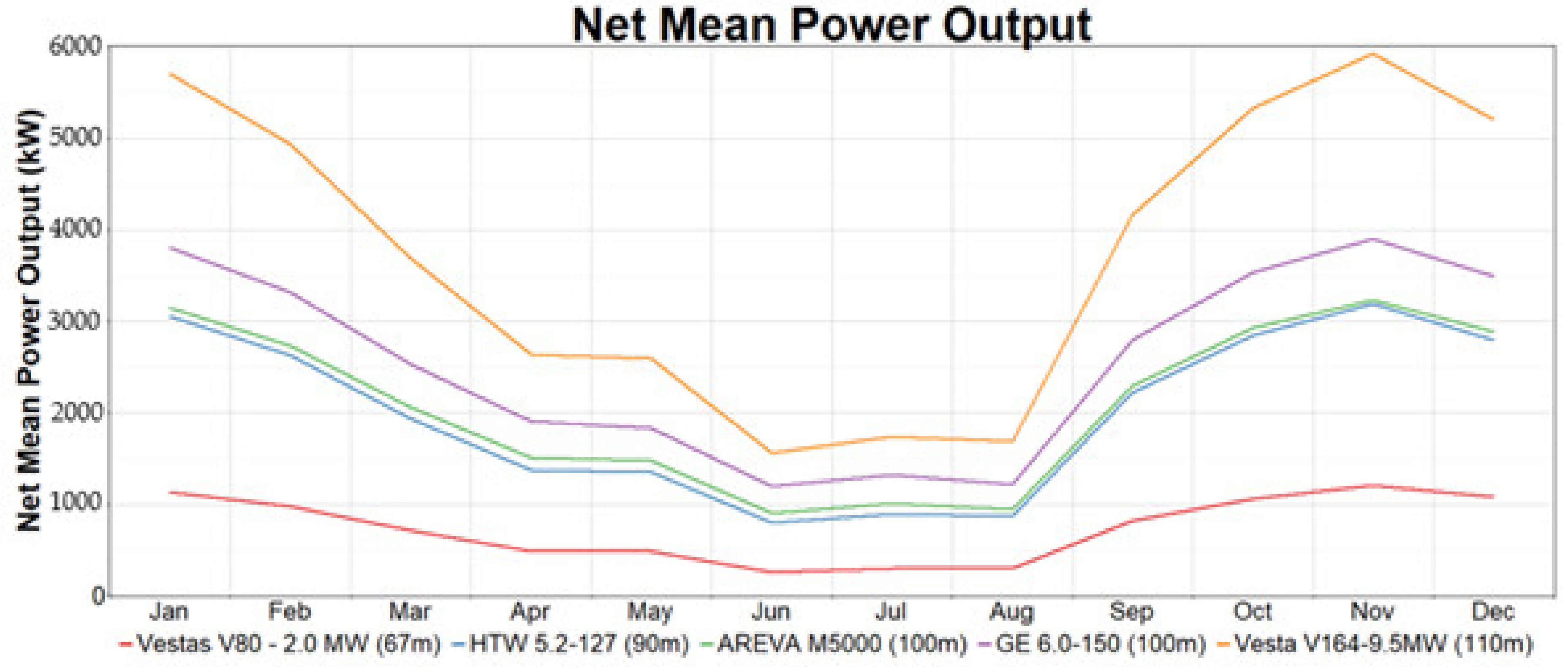
Figure 16.
Summarized monthly net capacity-factor profile conclusions.


Table 1.
Key parameters of wind distribution from met mast and MCP.
| Standard Deviation (m/s) | Wind-Speed Variation (m/s)2 | Mean Wind Speed (m/s) | Scale Factor (A) | Shape Factor (k) | |
|---|---|---|---|---|---|
| Met mast | 5.804 | 33.686 | 9.992 | 11.292 | 1.836 |
| MCP method | 5.751 | 33.074 | 9.0352 | 10.161 | 1.671 |
Table 2.
2019 Monthly net mean power output for five wind turbines.
| Net Mean Power Output (kW) | |||||
|---|---|---|---|---|---|
| Month | Vestas V80-2.0 MW (67 m) | HTW 5.2-127 (90 m) | AREVA Wind M5000-116 (100 m) | GE 6.0-150 (100 m) | Vestas V164-9.5 MW (110 m) |
| Jan | 1136.4 | 3059.9 | 3154.20 | 3814.5 | 5713.7 |
| Feb | 975 | 2624.2 | 2736.2 | 3322.2 | 4943.0 |
| Mar | 714 | 1936.4 | 2064.5 | 2537.5 | 3693.4 |
| Apr | 483.1 | 1379.2 | 1509.6 | 1903.2 | 2643.8 |
| May | 482.9 | 1358.0 | 1474.5 | 1838.1 | 2598.7 |
| Jun | 258.4 | 798.6 | 905.5 | 1191.7 | 1564.0 |
| Jul | 295 | 891.2 | 1013.6 | 1323.6 | 1737.8 |
| Aug | 303.1 | 875.3 | 950.1 | 1216.7 | 1683.1 |
| Sep | 821.2 | 2218.7 | 2297.9 | 2795.5 | 4166.9 |
| Oct | 1063.1 | 2853.4 | 2929.8 | 3542.9 | 5333.3 |
| Nov | 1208.1 | 3195.5 | 3237.3 | 3902.2 | 5932.1 |
| Dec | 1080.8 | 2796.5 | 2885.5 | 3496.3 | 5208.2 |
Table 3.
2019 Net capacity factors for five wind turbines.
| Net Capacity Factor (%) | |||||
|---|---|---|---|---|---|
| Month | Vestas V80-2.0 MW (67 m) | HTW 5.2-127 (90 m) | AREVA Wind M5000-116 (100 m) | GE 6.0-150 (100 m) | Vestas V164-9.5 MW (110 m) |
| January | 56.82 | 58.84 | 57.64 | 63.58 | 59.99 |
| February | 48.75 | 50.47 | 49.56 | 55.37 | 51.89 |
| March | 35.70 | 37.24 | 36.11 | 42.29 | 38.78 |
| April | 24.15 | 26.52 | 24.85 | 31.72 | 27.76 |
| May | 24.15 | 26.11 | 24.96 | 30.63 | 27.28 |
| June | 12.92 | 15.36 | 13.89 | 19.86 | 16.42 |
| July | 14.75 | 17.14 | 15.38 | 22.06 | 18.24 |
| August | 15.15 | 16.83 | 15.96 | 20.28 | 17.67 |
| September | 41.06 | 42.67 | 42.00 | 46.59 | 43.75 |
| October | 53.15 | 54.87 | 54.00 | 59.05 | 55.99 |
| November | 60.41 | 61.45 | 60.51 | 65.04 | 62.28 |
| Decemebr | 54.04 | 53.78 | 52.48 | 58.27 | 54.68 |
| Overall | 38.42 | 40.19 | 39.04 | 44.73 | 41.36 |
Publisher’s Note: MDPI stays neutral with regard to jurisdictional claims in published maps and institutional affiliations. |
© 2021 by the authors. Licensee MDPI, Basel, Switzerland. This article is an open access article distributed under the terms and conditions of the Creative Commons Attribution (CC BY) license (https://creativecommons.org/licenses/by/4.0/).
Share and Cite
MDPI and ACS Style
Hsu, W.-K.; Yeh, C.-K. Offshore Wind Potential of West Central Taiwan: A Case Study. Energies 2021, 14, 3702. https://doi.org/10.3390/en14123702
AMA Style
Hsu W-K, Yeh C-K. Offshore Wind Potential of West Central Taiwan: A Case Study. Energies. 2021; 14(12):3702. https://doi.org/10.3390/en14123702
Chicago/Turabian StyleHsu, Wen-Ko, and Chung-Kee Yeh. 2021. "Offshore Wind Potential of West Central Taiwan: A Case Study" Energies 14, no. 12: 3702. https://doi.org/10.3390/en14123702
Note that from the first issue of 2016, this journal uses article numbers instead of page numbers. See further details here.