Abstract
The drought that occurred in Zimbabwe in 2020 affected the country’s main hydro-power station causing the electricity supply to be less secure and reliable. This challenge resulted in load-shedding, which is not desirable to mining companies that require constant and reliable power for their operations. In that regard, a techno-economic analysis was carried out to assess the potential of integrating concentrated solar power (+thermal storage) and photovoltaics (+battery storage) to supply power at a typical mine in Zimbabwe. Two scenarios were simulated—a base case with no exports to the grid and another case where exports were allowed. The models were evaluated based on the generated renewable energy offsetting the demand from the mine, the energy exported, the grid contribution, the levelised cost of electricity and the net present value. The results show that the addition of a battery storage system to PV improves the percentage of the load offset by the renewable system and the generated energy by the renewable system by almost double. However, the installation cost, required land, LCOE, and simple pay-back also increased by approximately a factor of 2. The addition of a thermal storage system to CSP increased the generated energy, the capacity factor, and the renewable energy contribution by approximately a factor of 2. However, the land required for development and the installation costs also nearly doubled.
1. Introduction
According to the International Energy Agency, the mining sector consumes about 11% of the total worldwide energy [1]. By the year 2035, the demand for energy from mines (globally) is expected to increase by 36% [2]. However, the industry is currently powered predominantly by convectional energy sources which contribute to greenhouse gas emissions [2]. Several international mining organisations, which include but not limited to the International Council on Mining and Metals (ICMM), the Mineral Council of Australia, and the South African Chamber of Mines, agree that there is a need to improve the efficiency of their operations and to incorporate renewable energy systems to reduce greenhouse gas emissions from the industry [3].
The current power situation in Zimbabwe is not favourable for mining companies who require reliable power for their operations. According to the power utility first quarter figures for 2020, the generated electricity was approximately 20% short of the target [4]. This was mainly caused by the low levels of water in the Kariba dam which is the main hydropower station and technical challenges at one of the thermal power stations [4]. Mining companies are now compelled to look for alternative sources of power in case of load-shedding from the utility company. Renewable energy systems, particularly solar, have the potential to provide an alternative solution to this problem due to the generally good solar resources in the country [5].
Renewable energy systems such as Solar—Photovoltaic (PV) and Concentrated Solar Power (CSP)—and wind have matured enough to be economically competitive with power mining operations. The possibility of combining the systems with storage presents an opportunity to solve the challenge of intermittence of renewable energy sources, thereby providing predictable power. Thermal storage (in the case of CSP) and battery storage could be used as technological enablers to help renewable energy systems to provide reliable and dispatchable power. In addition, the hybrid renewable energy systems can have their dispatch automated to provide a high return on investments by supplying the lowest cost renewable electricity at any given time.
Currently there is not much research available to consider the possibility of powering mining operations using hybrid renewable energy systems. However, a significant number of scholars have evaluated quite diverse combinations of renewable systems to supply certain needs. Zurita et al. [6] evaluated the hybrid CSP and PV and battery energy system to supply a base load. One of the key results of the study was that integrating the battery storage would not make the system economically competitive. Parrado et al. [7] projected that the levelised cost of electricity (LCOE) of a hybrid PV–CSP system located in Chile in the year 2050. The results show that it is feasible to supply sustainable continuous electricity that could benefit industries such as mining. Green et al. [8] analysed the factors that are important to have a high-capacity factor from a CSP–PV hybrid system. The analyses concluded that there is a need for an effective configuration, a dispatch strategy and good sunlight to have a high-capacity factor from the system. Table 1 below shows some of the techno-economic analysis of renewable energy systems that exist in the current literature.

Table 1.
Selected techno-economic analysis of renewable energy existing in the literature.
Despite the high promise and potential of hybrid renewable systems, the question which still needs to be answered is whether the systems can reliably and practically provide power to the mining sector while providing economic benefits. Hybrid renewable energy systems in mining systems are still relatively new and off-takers have no first-hand experience of their ability to reliably provide power [3]. Another limitation facing the hybrid systems is related to amortisation. There is usually a mismatch between the life of the mine and the hybrid system asset life [3].
In this context, this paper intends to analyse and propose a renewable energy hybrid system that can be technically and economically integrated into mining operations. This report will help accelerate renewable energy integration in the mining sector in Zimbabwe through the following:
- Debunking the fear of renewable energy being intermittent by presenting cost competitive storage solutions that will lower the power supply disruption, which is something desired by mining companies.
- The report will present a reference point to which the mining community in Zimbabwe can consult and improve their expertise on the subject matter. For instance, there is not a single CSP plant in the country; hence, by explaining the technology and providing the energy yield studies thereof will be helpful.
- Showing that the capital costs of renewable energy systems are falling, which is something that has hindered the uptake of renewable energy in the country.
- Showing that the system can be profitable, hence providing an attractive option to investors and independent power producers.
The aim is to evaluate the potential of integrating CSP and thermal storage, and PV and battery storage systems to supply power at a mine in Zimbabwe. The chosen system should be configured carefully to meet the electrical demand of the mine during the period of most risk from load-shedding at the lowest cost possible.
Against this background, the remainder of the paper is structured as follows: the subsequent section gives a brief literature review about electrical usage in the mining sector and the background of CSP and PV systems in general. This is followed by a methodology section where the key performance indicators (KPI) are defined as well as the required technical and economic parameters for the models. Next, the results from the models are analysed based on the defined KPIs and compared with the literature. Lastly, the conclusion and the recommendations of the research are drawn by referencing the key outcomes, the study limitations, and future work to be completed.
2. Literature Review
2.1. Renewable Energy in the Mining Industry: An Overview
Population growth and urbanization has increased the consumption of goods and services which in turn leads to a higher demand for raw materials worldwide [13,14]. This has the effect of putting pressure on the mining industry as they attempt to meet this demand. The domino effect of this is increased energy consumption in the mining industry and greenhouse gas emissions. The global electricity consumption of the industry is 400 TWh of electricity a year [15,16]. Of this value, only 0.1% [15] is from renewable energy, except for large hydropower stations. The estimated greenhouse gas contribution globally from the mining industry ranges from 4 to 7% [17].
The mining industry is under pressure from decision makers, society, investors, and scientific experts to lower the carbon emissions and implement initiatives that will promote carbon neutrality [13,17]. Companies in this sector are seeking to achieve low carbon mining through energy efficiency measures and replacing fossil fuels with renewable energy [13,14,16,17,18,19,20]. The automation and the electrification of the processes and equipment that are powered by fossil fuels are considered to be solutions [17]. Liu et al. [19] discussed the potential of implementing energy storage systems—batteries and supercapacitors—and an energy management strategy for the operation of underground load-haul-dump vehicles. Annual installations of renewable energy (globally) in the mining industry have increased from 42 MW in 2008 to 3.4 GW in the year 2019 [14]. Table 2 below shows some of the mining companies in Africa that have integrated renewable energy.
Table 2.
Mining companies in sub-Sahara Africa that have integrated renewable energy.
Hybrid renewable energy has also proved to be beneficial to the mining industry [22]. According to a NREL report [14], most renewable energy systems installed between 2018 and 2019 in the industry were hybrids of wind, solar, energy storage, and other technologies complimented by fossil fuels to smoothen out the variability of renewable energy systems. Examples of hybrid systems have been installed in Australian mines. The Agnew gold mine installed 16 MW of wind power, 4 MW of solar power, and 13 MW of battery storage, and altogether contributed to 60% of the annual demand [23]. Moreover, the Green Smith mine has 27 MW of gas power, 8 MW of solar power, and 2 MW/1 MWh of battery storage [23]. There are plans in Africa to also build hybrid renewable energy systems. B2Gold’s Fekola mine in Mali plans to build 35 MWp and 17 MW of battery storage [24]. Bushveld minerals in South Africa plans to build 3.5 MW of solar PV and 1 MW/4 MWh of vanadium redox flow batteries [24].
The possibility of including hydrogen systems in the mining industry is also being considered. Kalantari et al. [20] investigated the possible use of hybrid renewable hydrogen energy as a solution to facilitate the absorption of renewable energy in the mining industry. The article proposes a combination of wind, battery, fuel cell, and thermal storage to meet 100% of the demand of a typical mine in Canada [20].
2.2. Drivers of Renewable Integration into Mining Industry
One of the main enablers for renewable energy integration in the mining industry is the reduction in energy costs and greenhouse gas emissions during operations [14,15,18]. Studies have shown that although the Capital Expenditure (CAPEX) of renewable technologies is higher than fossil fuel projects, their operational expenditure is significantly lower (especially for Solar PV) making them attractive when considering lifetime projects [15,16]. Off-grid mines, or those in the development stage are usually powered from diesel [17] which is affected by price volatility [14,16,18]. As with any other fossil fuel-based energy source, diesel is susceptible to tariff risks, exchange rates (it is usually imported), supply chain logistics, and geopolitics [14]. Renewable energy systems on the other hand will provide predictable energy costs and thus carry reduced risks from price intermittency [14,18]. Other drivers mentioned in the literature include:
- A reduction in carbon emissions [14,15,18];
- An improvement in the reputation of the company [15];
- Possibilities to repurpose the land used by the mining industry [18].
2.3. Constraints for Renewable Energy Integration into Mining Industry
One of the barriers in renewable energy integration into the mining industry is security of supply [15]. Due to their intermittent nature, the question that needs to be answered is whether the renewable energy systems can power typical 24 h mine operations matching the load profile [15]. There is also the need for technology proof-of-concepts [14]. Renewable technologies such as concentrated solar power (CSP) and energy storage need to be tested in mining environments to boost the confidence of industry players. A study by Gangazhe [25] reported that the lack of technical and economic feasibility in case studies of battery storage is a major barrier to their uptake in South Africa. From a financial perspective, there is usually a mismatch between the life span of the mine and the time necessary to recoup the capital investment [14,15,17]. Other barriers mentioned in the literature include:
- A lack of renewable energy awareness and expertise in the industry [14];
- Land constraints [14];
- The duration of power purchase agreements—mineral price volatility [15];
- A higher pay-back time for technologies such as CSP [15].
2.4. Sizing and Optimization of Hybrid Renewable Energy Systems
Optimal models need to be developed in order to use the available renewable energy economically and efficiently [17]. To build these models, the meteorological data, the technical specifications of the energy system, and the load profile need to be known. The optimization objectives must be determined and attained using either single objective optimization or multi-objective optimization [17]. The objectives can include technical parameters (such as renewable energy contribution), economical parameters (such as pay-back time), and environmental parameters (such as carbon dioxide savings) [17,26,27].
Optimization can be achieved by using software applications or traditional algorithms [17,28,29]. Commercial software applications that can be used include Homer, iHOGA, SAM, TRNSYS, and RETScreen [27,28,29]. Traditional algorithms include iterative approaches and artificial intelligence [28,29]. Saisandeep et al. [27] analysed the techno-economic performance of hybrid renewable electrification systems for remote villages in India. The technical performance of the system was optimized using the highest renewable fraction and the lowest unmet load percentage while the economical parameters were the minimal cost of energy and the lowest net present cost. The analysis was carried out using the Homer software tool [27].
3. Methodology
3.1. Model Description
The techno-economic models for PV, PV and Battery, CSP, and CSP and Thermal Energy Storage (TES) systems were developed for a typical mining load in Zimbabwe. The evaluation was based on the technical and economic performance using the System Advisor Model (SAM) software. The SAM software was used as it can make performance predictions and can estimate the energy costs for grid connected systems referencing the installation and operations cost, and the design parameters inputted to the model [30]. The methodology and key performance indicators used were based on similar analyses found in the literature review. Beuse et al. [31] described the general model required when performing a techno-economic assessment for PV and storage projects. The model should be inputted with data which include:
- Site specific data—for instance, the load profile;
- Technical parameters—efficiency, degradation;
- Commercial parameters—CAPEX, OPEX;
- Electricity tariff parameters—time of use of the tariff.
For the performance comparisons of the different renewable energy systems, Al-Ghussian et al. [9] used the following indicators:
- Levelised Cost of Electricity (LCOE);
- Renewable energy contribution;
- Net present value;
- Pay-back period.
Table 3 below describes the process taken.
Table 3.
Methodology.
The mentioned systems will be evaluated based on key performance indicators (KPI) listed in Table 4 below.
Table 4.
Key performance indicators used for evaluation.
3.2. Candidate Mine
3.2.1. Geographic Location
The Mimosa mine is a platinum group metal (PGM) and base metal mining company located in the Wedza sub-chamber of the Great Dyke of Zimbabwe (24 km west of Zvishavane town). The figure below (Figure 1) shows the geographical location of the Mimosa mine on the satellite picture (geographical coordinates with latitude −20.33 and longitude 29.83). The mine carries out underground mining and metallurgical plant processing activities and has an estimated life of 30 years. The output commodities of the mine include platinum, palladium, rhodium, gold, nickel and copper.
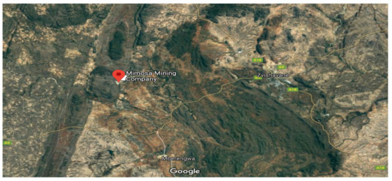
Figure 1.
Satellite location for Mimosa Mine (Source: Google maps).
3.2.2. Climate Data
The climate data used in this paper was sourced from Solcast. This is a data services company providing solar radiation data and solar forecasting globally using surface and satellite measurements [32]. Three sets of data were acquired—Typical Meteorological Year (TMY) in csv format, data customised for SAM software and PVSyst. Solcast data sets have been validated showing a 0% and 0.3% bias on Global Horizontal Irradiation (GHI) and Direct Normal Irradiation (DNI) data sets, respectively [32].
The Mimosa mine receives solar radiation of 2010 kWh/m2/year of DNI and 2034 kWh/m2/year of GHI according to the Solcast data. The DNI value shows that within the site it is technically feasible to develop CSP, as the minimum average value required is between 1900 and 2000 kWh/m2/year [32]. Figure 2 below shows the variation between the monthly GHI and DNI for the candidate site—the site receives higher DNI values than GHI between April and September.
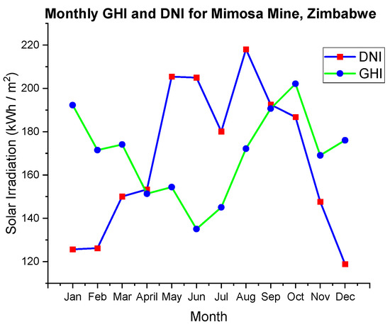
Figure 2.
Monthly GHI and DNI for the Mimosa mine.
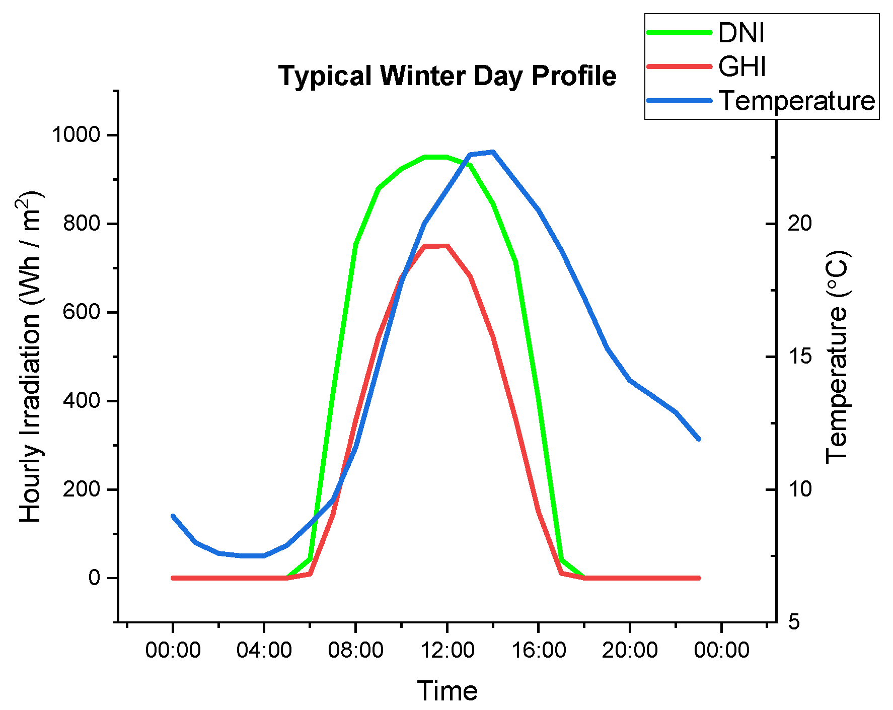
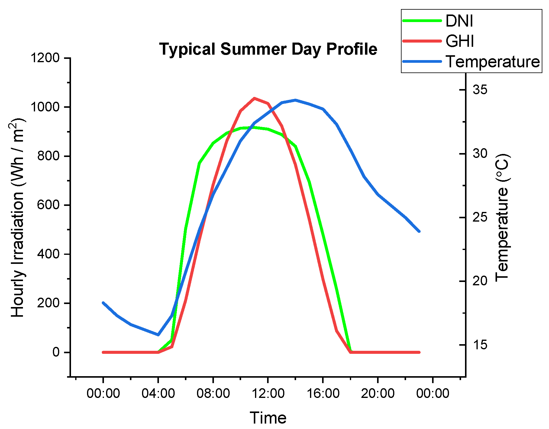
The two figures below (Figure 3 and Figure 4) show the typical hourly variation of DNI, GHI and the temperature during a day in summer and winter at the candidate site. For both figures, the GHI and DNI peak occurs around midday. The temperature in winter is below 25 °C which could help the PV system to perform better. However, the temperature in summer has a peak value of 35 °C which could affect the performance of the PV system.
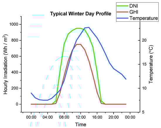
Figure 3.
Typical Winter Day Profile.
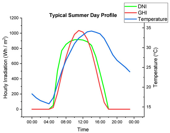
Figure 4.
Typical Summer Day Profile.
3.2.3. Mimosa Mine Demand Profile
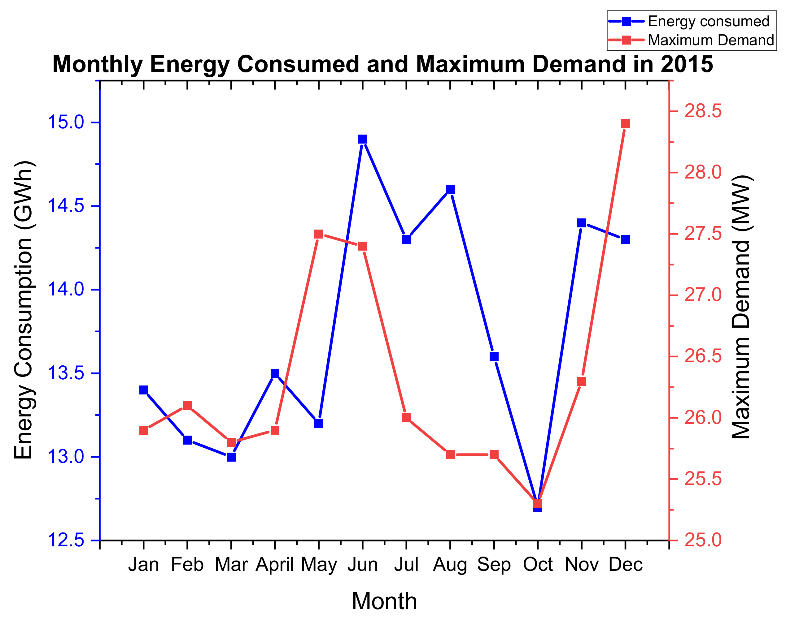
The mine is grid connected with an annual consumption of 165 GWh according to 2015 figures. The peak demand in that year was recorded in December with a value of 28.4 MW. Figure 5 below shows the monthly variation of the consumed energy and the corresponding peak power. The energy consumption graph has a minimum value of 12.7 GW (in October) and a maximum value of 14.9 GW in June. There is a variation from month to month of the energy consumed due to maintenance activities. For example, in October there was 5-day plant shut down (planned maintenance) which corresponded to the minimum monthly energy consumed that year.
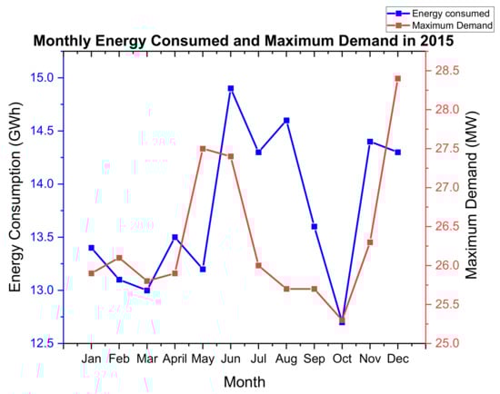
Figure 5.
The 2015 monthly energy consumption and maximum demand for the Mimosa mine.
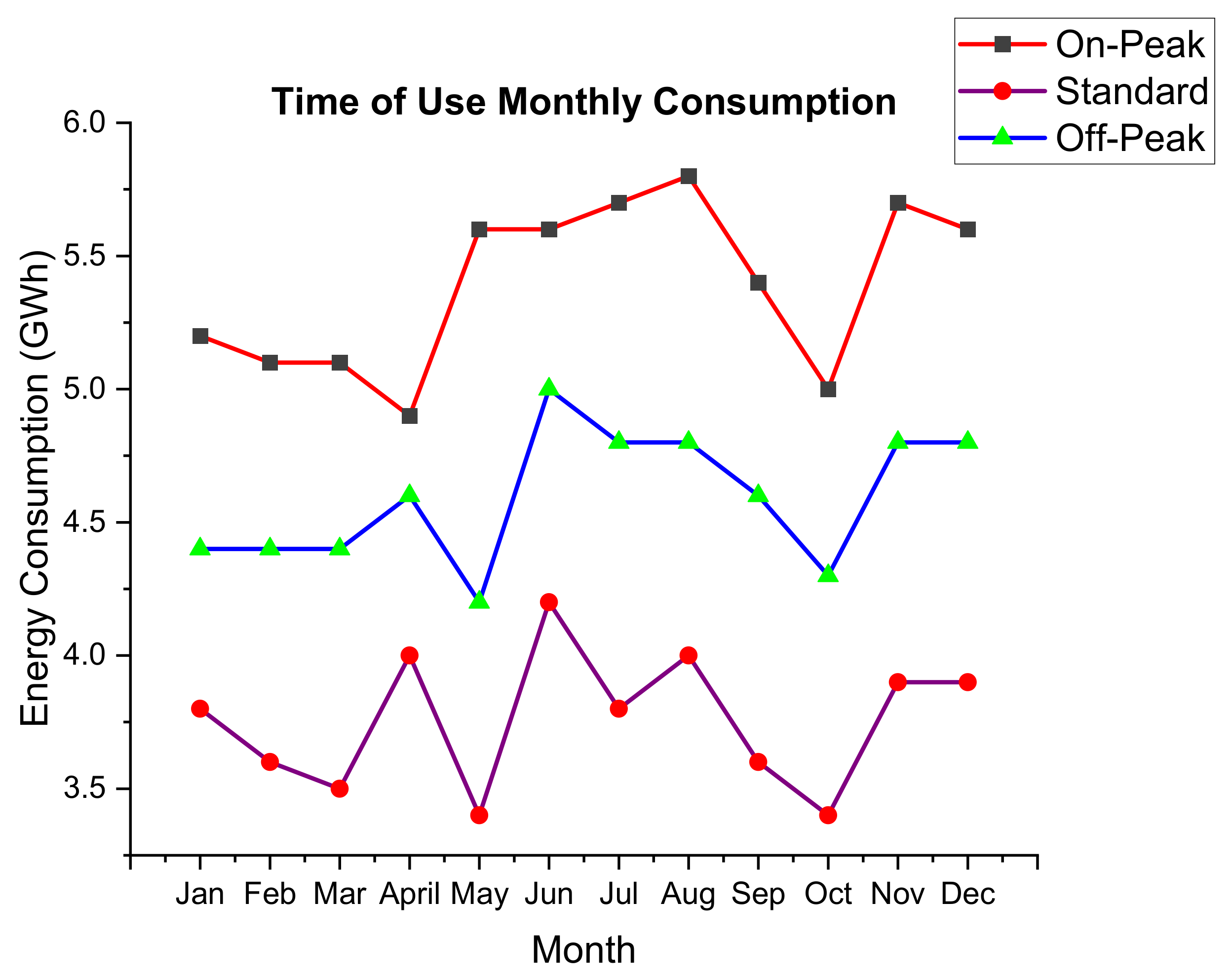
The data for the year 2015 shows that the mine consumed most of its energy during peak hours as shown in Figure 6 below. Table 5 shows the time periods of on-peak, standard and off-peak with the corresponding time of use of the tariff. The off-peak tariffs show that the mine could benefit by load shifting to off-peak hours and by finding an alternative cheaper source of electricity during the peak hours.
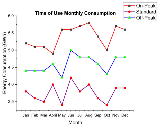
Figure 6.
Time of Use monthly consumption of the Mimosa mine in 2015.
Table 5.
Time of use periods and corresponding tariff.
The 2015 mine consumption figures show that 40% of the load was consumed during peak times and this translates to a high annual electricity bill. In addition, the electricity bill also includes the maximum monthly demand charge of USD2.6 per unit demand. The maximum demand charge is applied only during the peak and standard periods to encourage customers to load shift wherever possible and not strain the system.
Lately, Zimbabwe has been facing power shortages which have resulted in load-shedding, with the highest shedding period between 4 p.m. and 9 p.m. Such a scenario causes the mine to add another charge on the electric bill—an uninterrupted demand charge of USD1.95 per unit demand on each hour of the load-shedding. This shows that the mine can benefit from integrating reliable energy systems that can offset or eliminate grid energy consumption during these risk hours. The peak period is also coincidentally the high-risk period in terms of load-shedding.
3.3. PV System Design (Base Case)
3.3.1. Plant Capacity
A PV plant differs from convectional electrical systems because its performance is naturally connected to the unique details of the site and the specifics of the plant design. This makes it very difficult to calculate the required capacity of the plant. The equation used to calculate power in the HOMER software was utilised to estimate the rated capacity of this project [33]. The rated capacity assumes that the modules are operating at Standard Test Conditions (STC).
where:
- Power = peak load/demand required (from load profile)
- Rated capacity = unknown
- Net incident radiation = incident radiation at STC = 1000 W/m2 (assumption)
- Derating factor = 0.77 [34]
The recommended DC to AC ratio (form factor) to avoid inverter clipping losses is between 1.0 and 1.1 [35]. The proposed form factor for the project is 1.05. The tilt angle, azimuth angle and interrow space will be optimised through parametric analysis based on the energy produced and the LCOE. The key technical parameters used for the model are given in Table 6 below.
Table 6.
Technical parameters for the PV plant.
3.3.2. Financial Inputs for PV System
The commercial model was used to simulate the financial analysis of the PV system in SAM. This model assumes that the PV system will be developed, owned, and operated by the entity, and in this case, the Mimosa mining company. With this model, the entity will be able to buy and sell power at retail price. The metering and billing method used for this analysis was the net metering. This allows the PV system to supply the load with the shortfall supplied from the grid. However, this type of system also means excess generation of the system will be fed into the grid; hence, there is a need to design it in such a way that there is a reduced excess generation. For the base case scenario, the excess generation will be curtailed based on the assumption that there is no agreement with the utility company to export power. The grid energy charges are based on the time of use for the weekday as defined in Table 5 above in Section 3.2.3.
Table 7 below shows the parameters used in the model to calculate the LCOE, net present value (NPV) and pay-back period. The formulas describing how these are calculated in SAM are presented in Appendix A.
Table 7.
Commercial parameters for PV module. Adapted from [36].
3.4. PV + Battery System Design (Base Case)
3.4.1. Capacity Design
The PV and battery system in the model mainly aims to perform time of use arbitrage and to reduce the risk of losing the grid power due to load-shedding (or paying an uninterrupted charge). The AC connected behind the meter battery utilises the energy produced by the PV system during the day and discharges it during peak periods. The two main design parameters for the PV and battery system are:
- Power to Energy ratio—this determines the battery storage hours;
- PV size ratio—PV and battery plant capacity to PV (without storage) capacity. This determines the capacity of the PV plant to service both the load and the battery.
A parametric analysis will be carried out to optimise the design parameters based on the return on investments (net present value) and the ability of the system to supply the load during the period at most risk from load-shedding to a typically good day for PV production. From the load profile, the maximum energy required between 4 a.m. and 9 p.m. is 138 MWh (occurring in June) and this will be used to calculate the minimum required battery capacity [37]:
where:
- Ecap-min = minimum battery capacity;
- Ereq = peak energy consumption between 4 p.m. and 9 p.m. (inclusive) from load profile;
- D = days of anatomy (1 will be used for estimation with parametric study to determine the final);
- DOD = depth of discharge (80% will be used) [38].
Therefore, the minimum battery capacity for this model is 190 MWh with a rated power capacity of 30 MW (based on the peak demand of 28.4 MW). The technical parameters used to model the battery are given in Table 8 (the PV plant will use the same parameters as described in the above Section 3.3.1).
Table 8.
Battery technical properties. Adapted from [30].
3.4.2. Battery Dispatch
A manual dispatch will be defined in SAM so as to input specific time frames, other than using the automatic peak shaving dispatch. The battery will only be allowed to charge from the PV system (not from the grid) and can only discharge during peak or standard period times (7 a.m.–9 p.m.). The power generated from the PV system will prioritise the load first and will only charge the battery when the generated PV is greater than the load. Just as with the PV system, the excess generated power will not be exported to the grid and will be reported as a loss. In case the power from the PV and the battery is not enough to supply the load, the grid power will be used instead.
3.4.3. Economic Inputs to PV and the Battery System
The commercial model used for this system is the same as the PV system described in Section 3.3.2 above. Table 9 below shows the economic parameters for the battery system to calculate the LCOE, the net present value, and the pay-back period (for PV they are the same as described in the previous Section 3.3.2).
Table 9.
Economic parameters for battery storage. Adapted from [36].
3.5. Concentrated Solar Power (CSP) System Design (Base Case)
The system chosen for primary analysis in this project is the parabolic trough CSP system. Based on the literature review, this is a more mature system (when compared to other CSP systems), with commercial operational plants around the world including in Africa.
3.5.1. System Design
The recommended methodology to design and model a parabolic trough CSP plant in SAM is given below [30]:
- Define the solar field design parameters;
- Configure the receiver and collector components;
- Determine the transport operational limits;
- Configure the loop;
- Specify the power cycle design point;
- Update the cost and financials;
- Optimise uncertain parameters—solar multiple, storage hours.
Table 10 below shows the technical parameters used to develop the CSP parabolic trough system for this project. The details of the most important parameters are described below.
Table 10.
Technical parameters for CSP. Data from [30].
Design Point DNI
This is used to calculate the aperture area required to drive the power cycle at its design capacity [30]. Theoretically, the value should be close to the maximum DNI value of the site. A low DNI value results in excessive dumped energy while a high reference DNI value results in an undersized solar field that can only operate at the designed capacity a few times [30]. A parametric analysis will be used to determine the design point DNI.
Solar Multiple (SM)
This is defined as a multiple of the aperture area required to operate the power cycle at its design capacity [30]. An SM value of 1 defines an aperture area that will generate (when exposed to solar radiation equivalent to the design point DNI) the thermal energy required to drive the power block at its rated capacity. A parametric analysis will be used to determine the optimal SM for this application.
Design Turbine Gross Output
This is the power cycle’s design output (not including parasitic losses) that is used to determine the solar field area [30]. The value is determined from the maximum load required. The maximum load from the demand profile is 28.4 MW; hence the net estimated output at the design capacity is 29 MW. The gross turbine output is determined using the following equation:
Table 10 below shows most of the specifications used to model the parabolic trough CSP system in SAM.
3.5.2. Economic Parameters for CSP
The commercial model used for this system is the same as the PV system described in Section 3.3.2 above. Table 11 below shows the economic parameters for the CSP system to calculate the LCOE, the net present value and the pay-back period.
Table 11.
Economic parameters for CSP. Data from [39].
3.6. CSP + Thermal Energy Storage (TES) System Design (Base Case)
3.6.1. Capacity Design
Just as with the PV and battery system described in Section 3.4, the main aim of adding thermal energy storage is to assess the potential of performing time of use arbitrage and reducing the risk of losing grid power due to load-shedding (or paying the uninterrupted charge). The storage hours of the system and the solar multiple are the two main design parameters of the CSP and TES system. A parametric analysis will be carried out to optimise the two design parameters based on LCOE and the ability of the system to supply the load during the risk period of load-shedding on a typically good day for CSP production.
Besides the solar multiple, the CSP and TES will utilise the CSP technical and commercial parameters as described in Section 3.5. A direct system where molten salts are used both as a heat transfer fluid and storage will be utilised for this project because of their improved efficiency advantage over the indirect system. Table 12 below describes how the TES technical (and economic) parameters will be utilised.
Table 12.
TES technical and economic parameters. Data from [30].
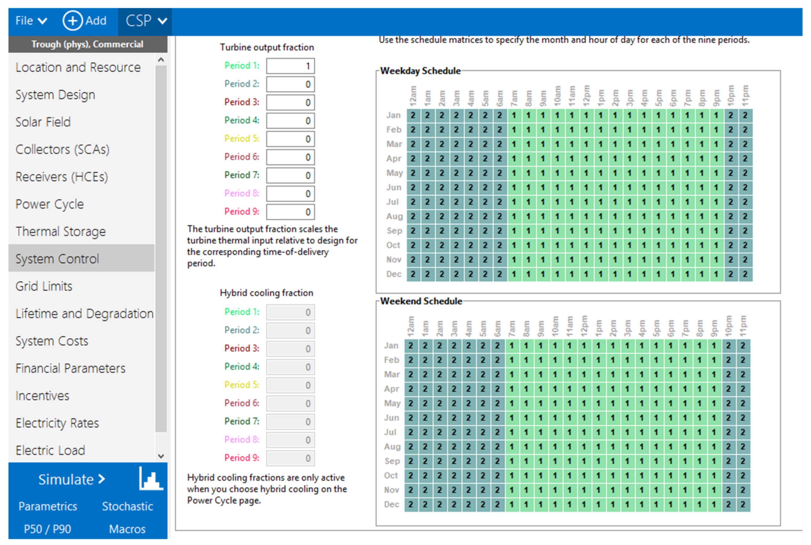
3.6.2. Dispatch Control
The CSP and TES system will dispatch energy from 7 a.m. to 9 p.m. (peak and standard periods) with the off-peak period (11 p.m. to 6 a.m.)—when the tariff is cheap—left for the grid alone. Figure 7 below shows the dispatch control for the system implemented in SAM—period 1 shows when CSP + TES can dispatch power to the load with the grid power able to fill in the shortfall while period 2 shows that the system output will be zero, hence the grid covering the load alone.
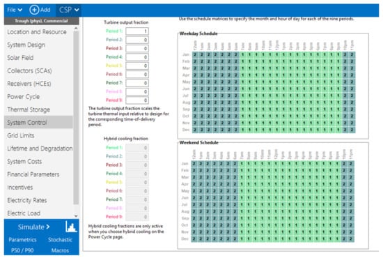
Figure 7.
Dispatch control for CSP and TES in SAM.
3.7. Evaluating System with Exports
3.7.1. Technical Consideration
The current transmission line supplying the mine is rated at 132 kV, 100 MVA feeding into 2 × 20 MVA, 132 kV/11 kV transformers connected in parallel. The maximum demand (according to 2015 figures) at the mine is 28.4 MW. Taking these figures into consideration, the grid exports from the renewable system will be limited to 60 MW for this analysis. Table 13 below shows the procedures taken to analyse the systems.
Table 13.
Methodology to simulate system with exports.
3.7.2. Economic Consideration
The financial model to be used in this section is net billing. In SAM, the net billing is calculated by subtracting the generated energy from the load in each simulation time step over a month. For months with an excess generation, the dollar value of the excess energy is credited to the month’s bill with the value of the credit determined by the sale rate. The practical procedure to determine the sale rate is through a power purchase agreement with the utility provider. However, for this analysis, an assumption will be made to equate the sale rate and the time of use of the tariff as described in Section 3.2.3.
4. Results
4.1. PV System Results
4.1.1. Tilt Angle Optimisation
A parametric study was performed to determine the optimum tilt angle for the site. The Figure 8 below shows the variation in the annual energy produced and the LCOE for a 37 MW DC PV plant with a tilt angle. The annual energy increased with a tilt angle increase (0–20°) from 53.1 GWh to 55.1 GWh. Once the tilt angle was greater than 20°, the annual energy started to decrease. The curve for LCOE is a mirror image of the annual energy with its lowest value (US$0.048/kWh) at tilt angle of 20°. This result is consistent with the literature review which pointed out that the latitude of the site is usually the optimum angle, hence the tilt angle of 20° will be used in the model.
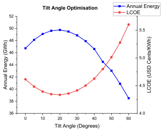
Figure 8.
Variation of the annual energy and the LCOE with a tilt angle.
4.1.2. Azimuth Angle Optimisation
The highest energy generated was found at an azimuth angle of 0° (north facing) and together with the lowest value of LCOE as shown in Figure 9 below. This is consistent with the literature review, which revealed that the best orientation for PV plants in the southern hemisphere should be facing the north.
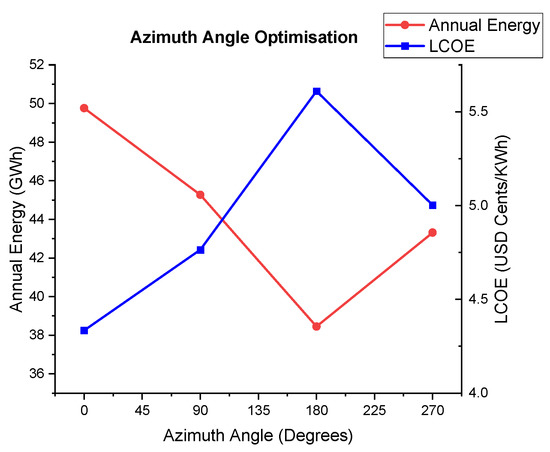
Figure 9.
Variation of the annual energy and the LCOE with an azimuth angle.
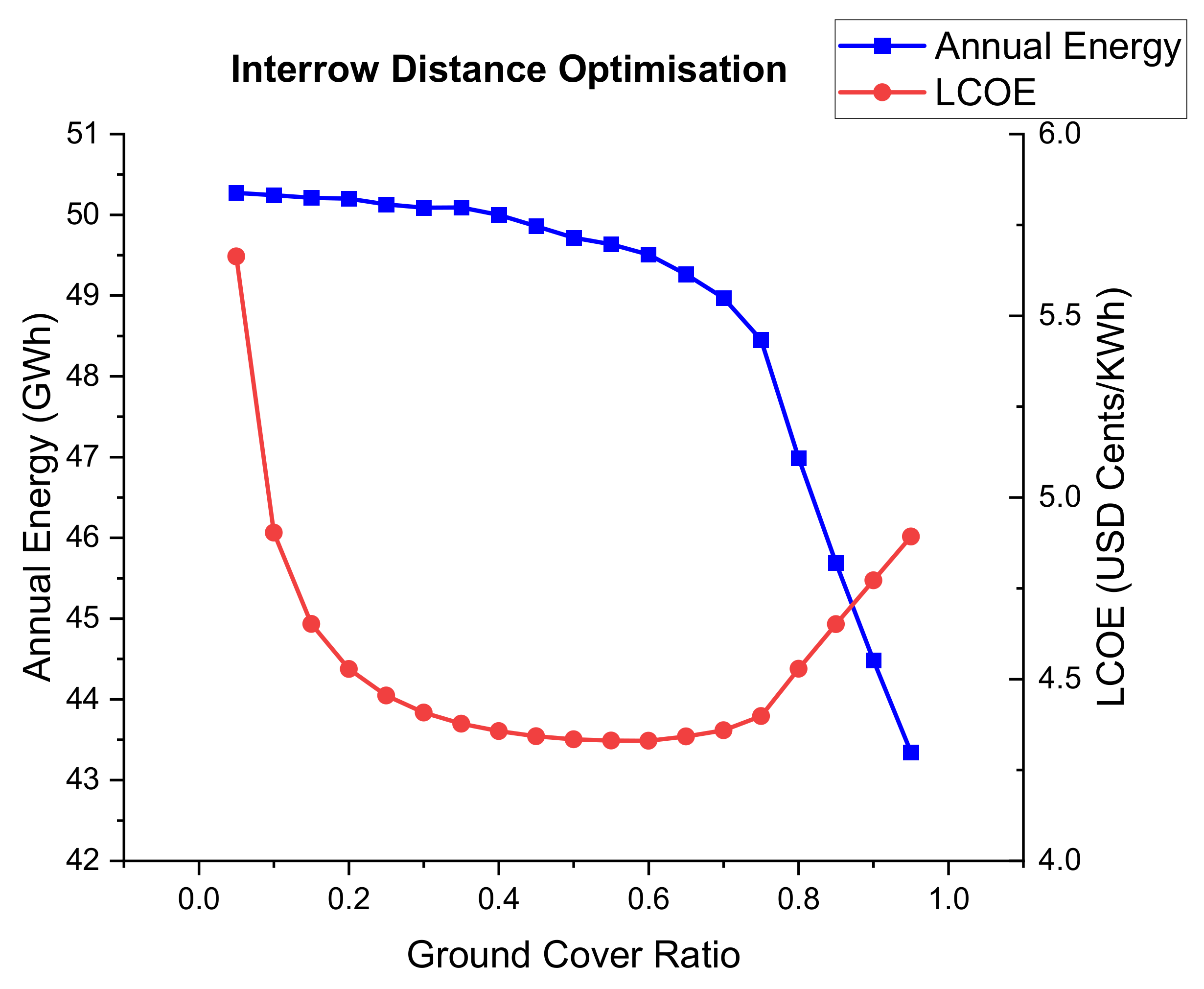
4.1.3. Interrow Distance Optimisation
The interrow distance is inversely proportional to the Ground Cover Ratio (GCR). This is defined as the area between the PV modules and the total ground area. Figure 10 below shows the variation in the annual energy generated and the LCOE with GCR. The annual energy generated shows that as the GCR reduced (hence the interrow distance increases) the annual energy increased steadily up to a GCR of 0.45 where it started to flatten out. This means the lower the interrow distance, the more chances there are of shading leading to reduced generated energy. As the interrow distance increases (GCR decreases), the generated energy will not vary much because the factor of self-shading will be eliminated.
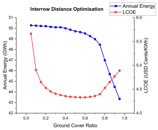
Figure 10.
Variation of the annual energy and the LCOE with the Ground Cover Ratio.
The LCOE in Figure 8, Figure 9 and Figure 10 above resembles a bowl or parabolic shape. Very low values of GCR (high values of interrow distance) have a high LCOE even though the generated energy is high. This is because the greater the interrow distance the more land area that is required, thereby increasing the installation costs. On the other hand, high GCR values (low interrow distance) mean more chances of self-shading, leading to reduced generated energy which increases the LCOE. The optimum GCR value is the point where the annual energy starts to flatten, showing that the interrow distance is now just enough to eliminate interrow shading. In this case, it is 0.45 giving an interrow distance of 2.4 m.
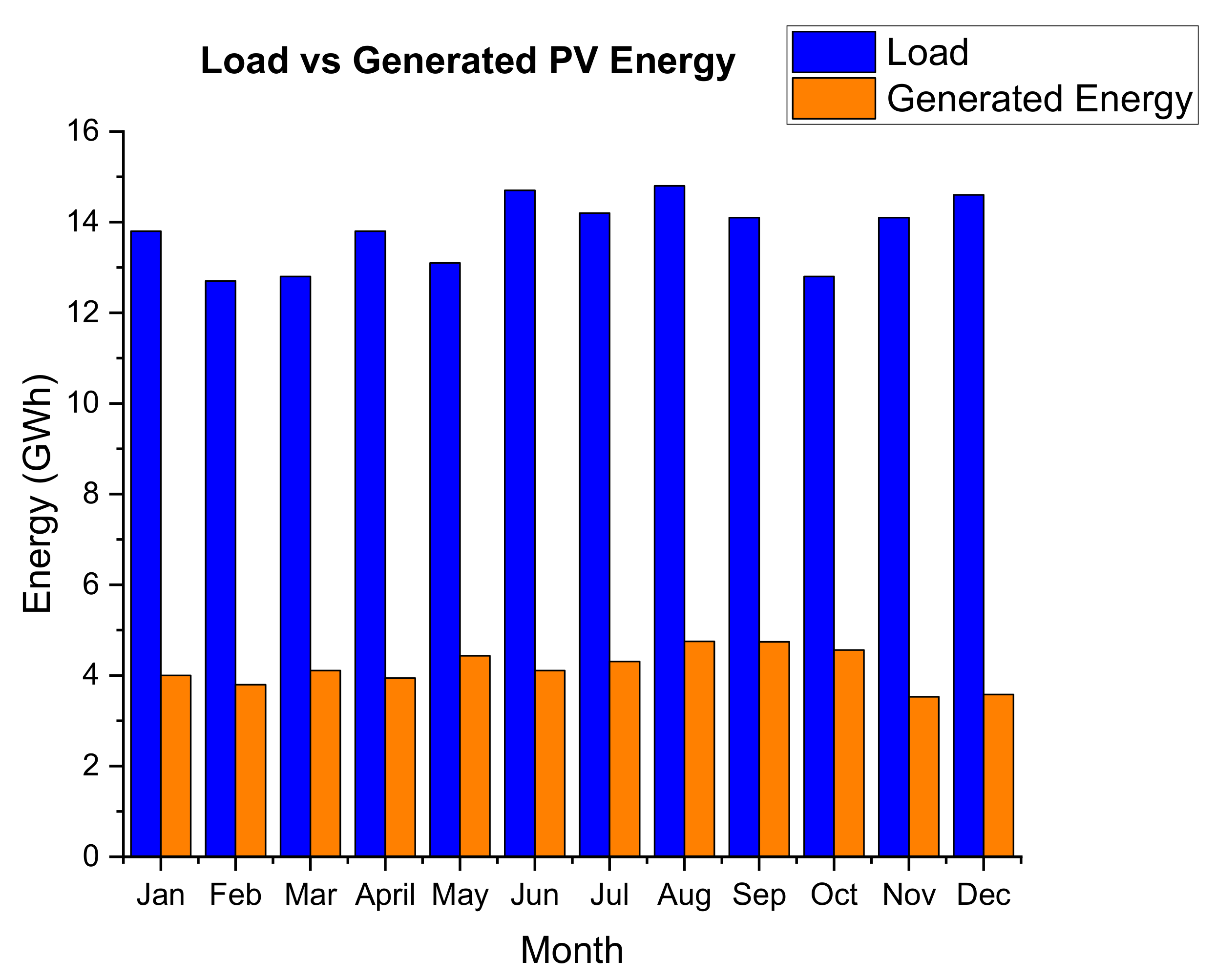
4.1.4. Technical Performance of Optimised PV Model
The simulation of the optimised 37 MW DC PV plant predicted an output of 55.13 GWh during the first year of operation. This is approximately 33.3% of the annual demand of the mine. Figure 11 below shows the monthly load vs. the generated PV energy. The graph for the generated energy shows limited seasonal variation due to the optimisation of the tilt angle.

Figure 11.
Monthly variation of load vs. generated PV energy.
The expected capacity factor of the PV plant in the first year is 19% which compares with the 2019 weighted average capacity factor according to the IRENA database [40]. The performance ratio of the plant is predicted to be 77% with major losses including soiling, module mismatch, and cable losses. The most significant loss however is that caused by the grid limit (generation exceeding load and no exporting power) which accounted for 10.3%.
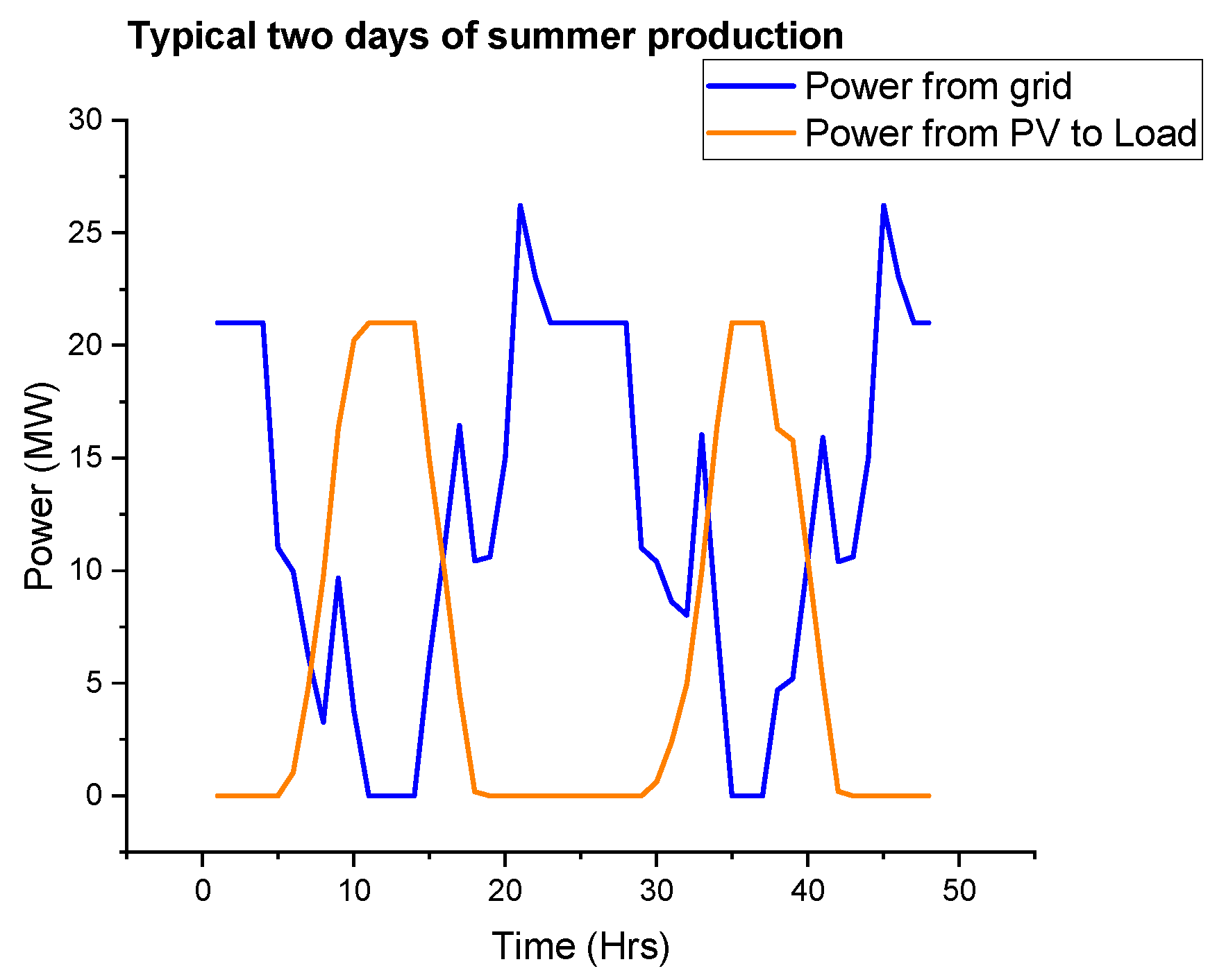
On a typically good PV production day, as shown in Figure 12 below, the PV plant is able to supply the mine load alone (on this day, 23 MW) for 4 h between 9 a.m. and 1 p.m. However, the morning spike is largely being covered by the grid because at the time it occurs (8 a.m.), there will not be enough irradiation. The graphs show that on a typically good day, the PV generated could be higher than the energy from the grid from 6 a.m. to 3 p.m. As expected, the load during the night is supplied from the grid.
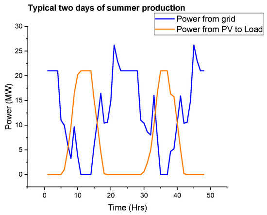
Figure 12.
Two typical consecutive days with good PV production.
4.1.5. Comparing PVSyst and SAM
For comparison purposes, the identical PV system (37 MWdc, 1.05 DC/AC ratio, same PV, and inverter efficiencies) was modelled in PVSyst, software version 6.43. The only adjustment that was made was on the grid limitation: the PVSyst allowed all the generated energy to be exported without limitation from the load profile (the same adjustment was made to the SAM model). The results show that the energy produced from the two software packages differed by only 1.65%, with the largest difference related to the performance ratio as shown in Table 14 below.
Table 14.
Comparison between PVSyst and SAM.
4.1.6. Economic Performance of Optimised PV Model
The installation cost of the project is predicted at USD 0.76 per DC Watt which is comparable to the projects completed in India in 2019 which had a weighted average installation cost of USD 0.62 per DC Watt [40]. Similarly, the predicted LCOE of this PV system is USD 0.048/kWh which is comparable to the weighted average LCOE of USD 0.045/kWh of the projects completed in India in 2019 [40]. The predicted net present value of the project is about USD 41 Million with a pay-back period of 5.1 years, reinforcing the economic viability of this project. Table 15 below shows the main economic indicators for this project.
Table 15.
Economic performance indicators for the PV system.
The first-year figures show that the annual energy electricity bill has been reduced from USD13.7 million to 8.02 million. This means that by reducing the annual load by about 33.3%, the system will be able to save about 41.4% of the annual electricity bill. The difference in the two numbers is caused by the fact that the PV System is offsetting the load during the peak and the standard tariff periods while the grid electricity is mainly used during off-peak hours. Figure 13 below shows the monthly electricity bill with the PV system and without.
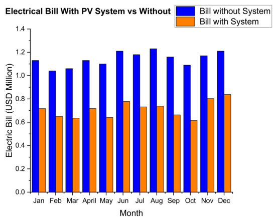
Figure 13.
Monthly electricity bill with the PV system vs. without.
4.2. PV + Battery Results
4.2.1. Battery and PV Plant Capacities Optimisation
A parametric analysis was carried out to determine the optimum storage hours (hence battery capacity) and the PV size based on the load profile, the desired operation and the return on the investment. The trend from Figure 14 below shows that in general, the smaller the PV plant and the lower the storage hours, the more viable the system. PV size ratios of 1.5 and 2 have a positive NPV value for the whole range of storage sizes simulated (2 h to 12 h) while the 2.5 PV size ratio is only viable for up to 9 h of battery storage. The PV size ratios from 3 to 5 are not viable for this designed application for all the simulated storage hours. For storage hours, the viability decreases with the increase in storage size. The 2 h storage battery has three viable PV sizes while the 12 h battery storage is only viable for two PV sizes.
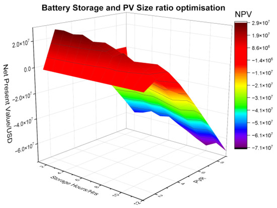
Figure 14.
Three-dimensional graph showing the battery and PV capacity optimisation.
To determine the optimum system for the model, the minimum storage required for the battery to supply the load during the high-risk load-shedding period must be considered. The calculated minimum battery capacity is 190 MWh which translates to about 5 h of storage (Using Equation (8) in Section 3.4.1). Using the graph above, the chosen battery storage capacity is 7 h, which translates to 210 MWh (30 MW × 7 h without considering DOD). This value is greater than the designed requirement of 190 MWh calculated in Section 3.4.1. For 7 h of storage, the PV ratio sizes of 1.5, 2, and 2.5 have a positive NPV value. The 2.5 PV size ratio was not chosen because the NPV value was significantly below for the other two sizes. Although the 1.5 PV size ratio has a slight better NPV value (by approximately USD 2 million), the PV ratio of 2 performed better in terms of the annual energy produced, and hence this ratio was chosen for the model.
The optimum combination chosen is:
- PV size ratio of 2 which translates to 2 × Peak power for PV without storage = 2 × 37 MW DC = 74 MW DC.
- Power to Energy ratio of 1:7 translating to 7 h of battery storage meaning a battery capacity of 210 MWh.
4.2.2. Technical Performance of the Optimised PV + Battery System
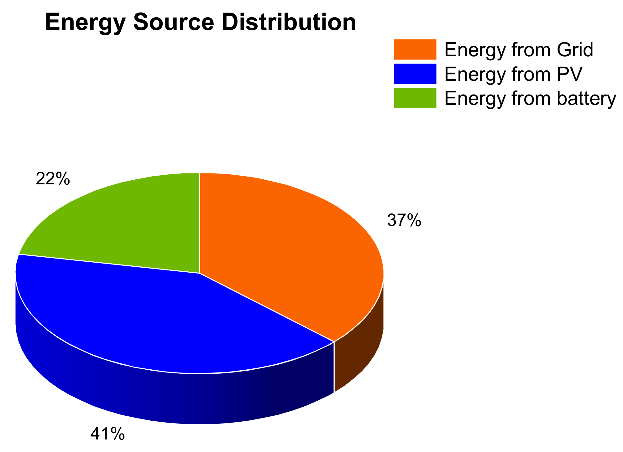
The simulation of the optimised 74 MW DC PV plant with 210 MWh of battery storage predicted an annual energy output of 103 GWh in the first year. This is approximately 63% of the annual mine load—41% from PV and 22% from the battery—as shown in the pie chart below (Figure 15). The design was meant to cater for the peak and standard periods which constitute about 68% of the load (from the load profile); hence, the system was 5% under the target with the grid covering the slack.

Figure 15.
Energy distribution of the PV and battery system.
The expected capacity factor of the system is 18.6% with a performance ratio of 75% and a battery roundtrip efficiency of 92.7%. The losses resembled that of the modelled PV with the addition of the battery losses. As with the PV system, the most significant loss is the grid connection limit with a value of around 13%.
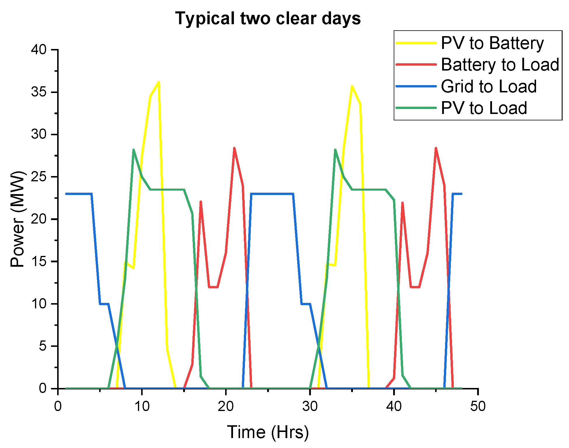
On a typically good day of PV production, as shown in Figure 16 below, the hybrid system is able to supply the load over the designed periods (peak and standard). The PV plant will supply the load alone from 7 a.m. to 2 p.m. The battery and PV plant will supply the load from 2 p.m. to 5 p.m. and then the battery will supply the load alone up to 9 p.m. The grid will then pick it up from 10 p.m. to 6 a.m. which is the off-peak period.
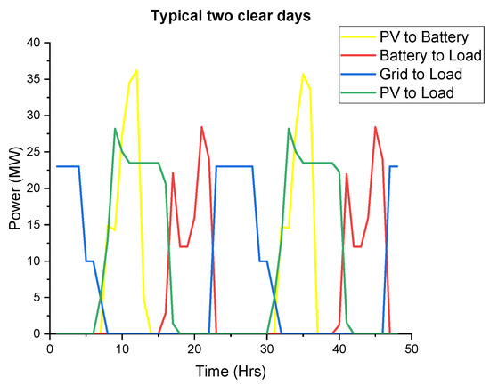
Figure 16.
Two typical consecutive days with good PV production.
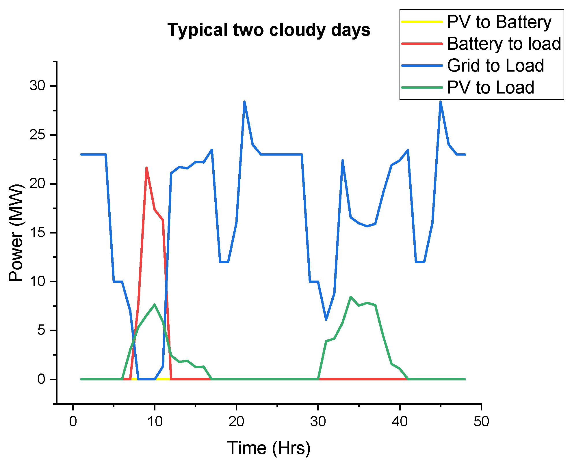
On a typically bad day (such as a cloudy day) for PV production, as shown in Figure 17 below, the PV and Battery system only covers the load alone between 7 a.m. and 10 a.m. on the first day of the period. The grid power will then be used thereafter with a little help from the PV plant the next day.
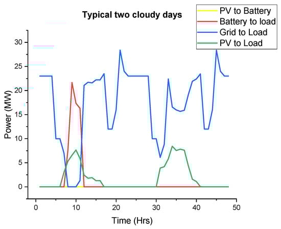
Figure 17.
Two typical consecutive days with bad PV production.
4.2.3. Economic Performance of Optimised PV and Battery System
The installed cost of the PV and battery system is USD 1.5/Wdc with the cost of storage contributing 43.3%. The LCOE of the system is USD 0.106/kWh—this is more than double than that of PV system alone. The predicted simple pay-back period is 10.8 years with an NPV value of USD 19.26 Million. Table 16 below shows the main economic indicators of the project.
Table 16.
Economic performance indicators for the PV and battery system.
The first-year simulation results show that the annual electric bill is reduced from USD13.7 million to USD 3 million. This represents about a 78% reduction in the electricity bill after offsetting 63% of the load. As with the PV system, the difference in the two figures is because the grid power is mainly used during the off-peak period which is cheaper than the periods covered by the PV and battery system. The graph below (Figure 18) shows the monthly electricity bill with PV and battery and without.
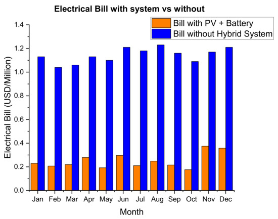
Figure 18.
Monthly electric bill with the PV and battery system vs. without.
4.3. CSP Results
4.3.1. Design Point Optimisation
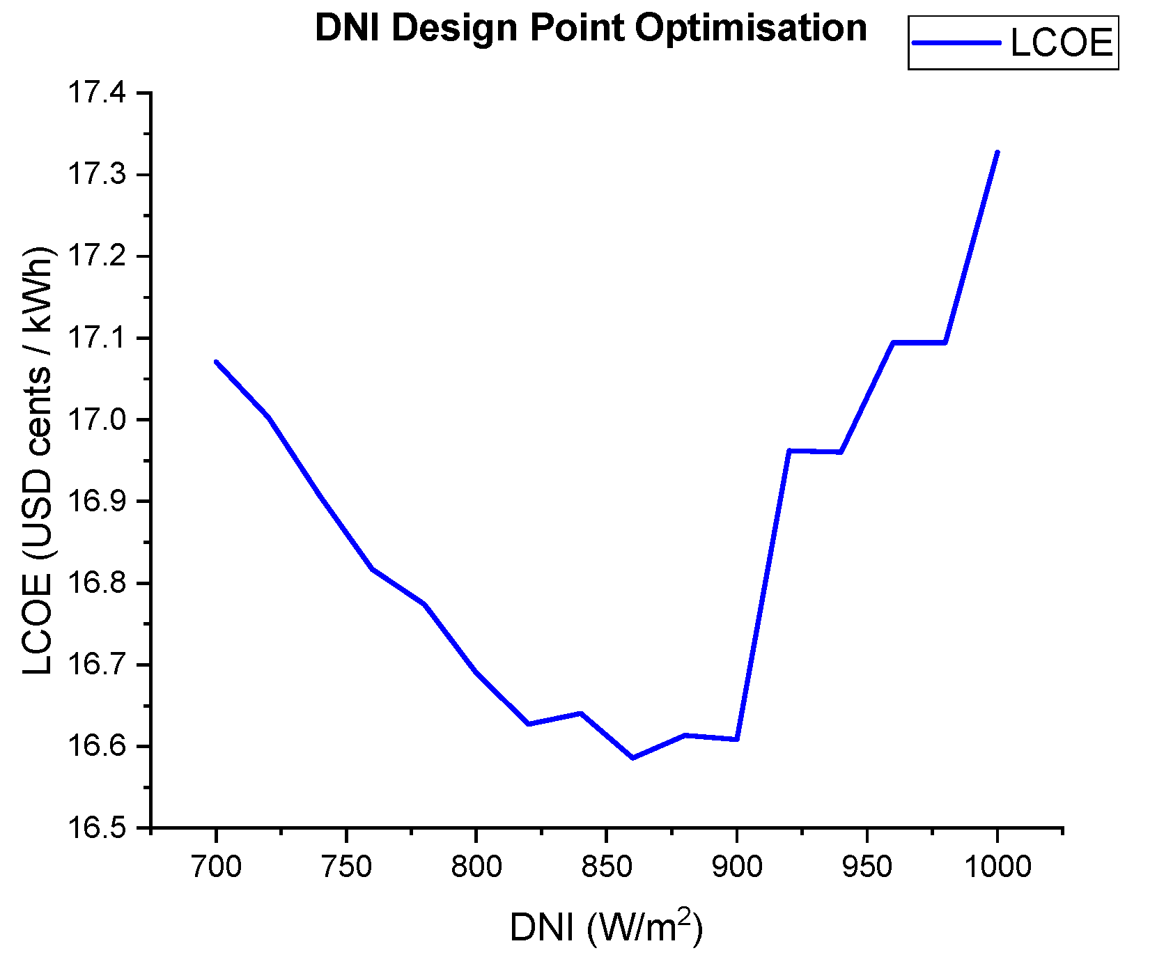
The graph below (Figure 19) shows the variation of the LCOE with the design point DNI with the minimum LCOE occurring at 860 W/m2. Values higher than this DNI have a high LCOE because the system is oversized and operates at the design capacity for a limited time only. Below 860 W/m2, the LCOE is higher (even though there is more generated energy) because the solar field area increases with a low design point DNI hence increasing the installation cost.
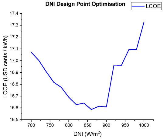
Figure 19.
Design point optimisation.
4.3.2. Solar Multiple Optimisation
The optimum solar multiple for the system from the graph (Figure 20) below is 1.25. This value is consistent with the literature review which revealed that a solar multiple of 1.3 is a typical optimum for a no storage CSP system [41]. Although values higher than the solar multiple of 1.25 produce higher energy values, the increase in land size increases the LCOE.
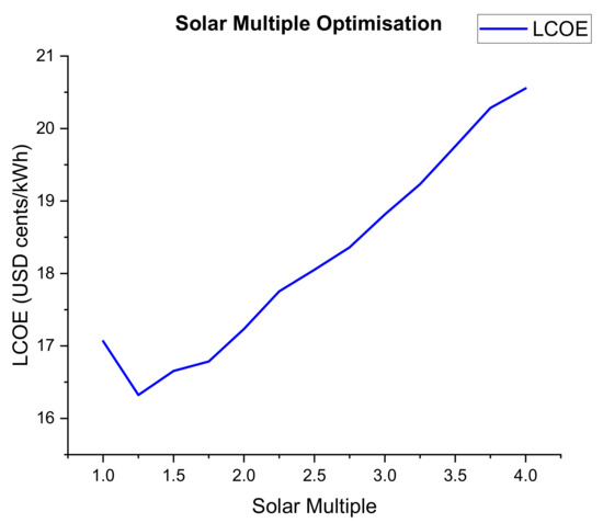
Figure 20.
Solar multiple optimisation.
4.3.3. Field Subsections Optimisation
The shape and location of the header piping delivering heat to the power cycle is determined by the number of field subsections. The orientation will directly affect the amount of heat loss in the pipes. The graph below (Figure 21) shows that the optimal number of subsections is two based on the lowest LCOE and highest generated energy.
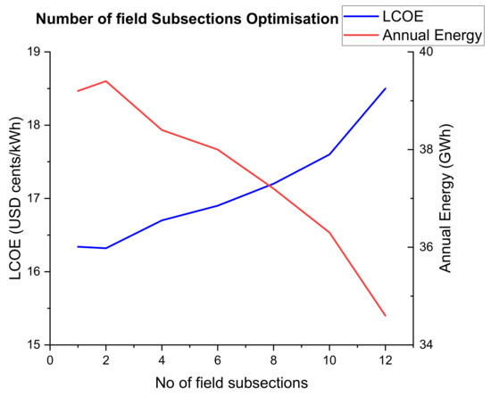
Figure 21.
Optimisation of the number of field subsections.
4.3.4. Technical Performance of the Optimised CSP
The simulation of the optimised 32 MW gross output, solar multiple of 1.25, and DNI design point of 860 W/m2 predicted a net annual electricity energy production of 39.3 GWh during the first year of operation. This is approximately 23.7% of the annual demand of the mine with a capacity factor of 20.6%. The predicted capacity factor compares with figures given in IRENA [41] for no storage CSP systems which has values ranging from 21% to 23%. Figure 22 below shows the monthly production of CSP energy vs. the monthly demand of the mine.

Figure 22.
Monthly generated CSP vs. the monthly demand.
On a typically good day for CSP production, as shown in Figure 23 below, the system is able to supply the load from 8:00 a.m. to 2:00 p.m. The grid power will start to compliment the CSP after 2:00 p.m. up until 4:00 p.m., where CSP production will fall to zero. From then on, the grid will supply the load up until the next day.

Figure 23.
Two typical consecutive days with good CSP production.
On a typical overcast day, as shown in Figure 24 below, the CSP system will absorb power from the grid (for auxiliary circuits) instead of generating power. The grid power will supply the load during the day and night.
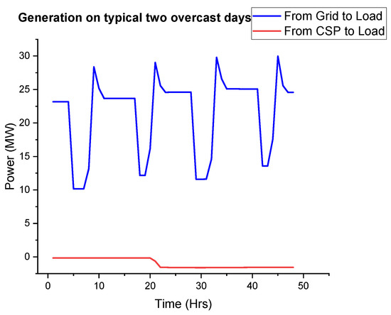
Figure 24.
Two typical consecutive days with bad CSP production.
4.3.5. Economic Performance of the Optimised CSP System
The installation costs of the system are predicted at USD 2479/kW. The IRENA renewable cost database for CSP commissioned in 2019 showed installation costs ranging between USD 3704/kW and USD 8645/kW—with the exception that these figures are for systems with storage, and hence are higher. The predicted LCOE of the system is US cents 16.32/kWh which is slightly lower than the weighted average of the LCOE (US cents 18.2/kWh) of the CSP system in 2019 [40]. However, the predicted NPV for the system is below zero making it unattractive option to invest. Table 17 below shows the main economic indicators of the system.
Table 17.
Economic performance indicators for the CSP System.
The first-year simulation figures show that the annual electricity bill is reduced from USD 13.69 million to 9.63 million. This represents a cost reduction of approximately 29.8% on the annual electric bill after offsetting approximately 23.7% of the annual load. Figure 25 below shows the monthly electricity bill with the PV system and without.
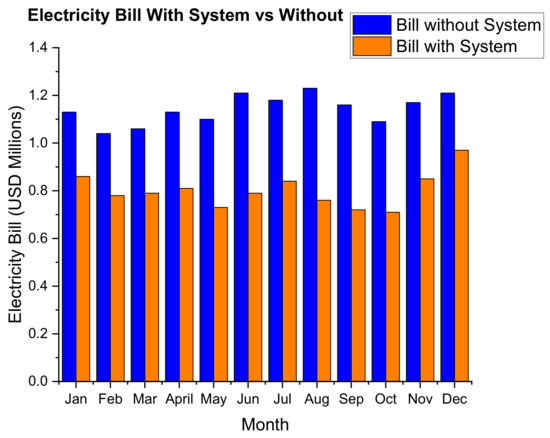
Figure 25.
Monthly electricity bill with the CSP system vs. without.
4.4. CSP + TES Results
4.4.1. Storage Hours and Solar Multiple Optimisation
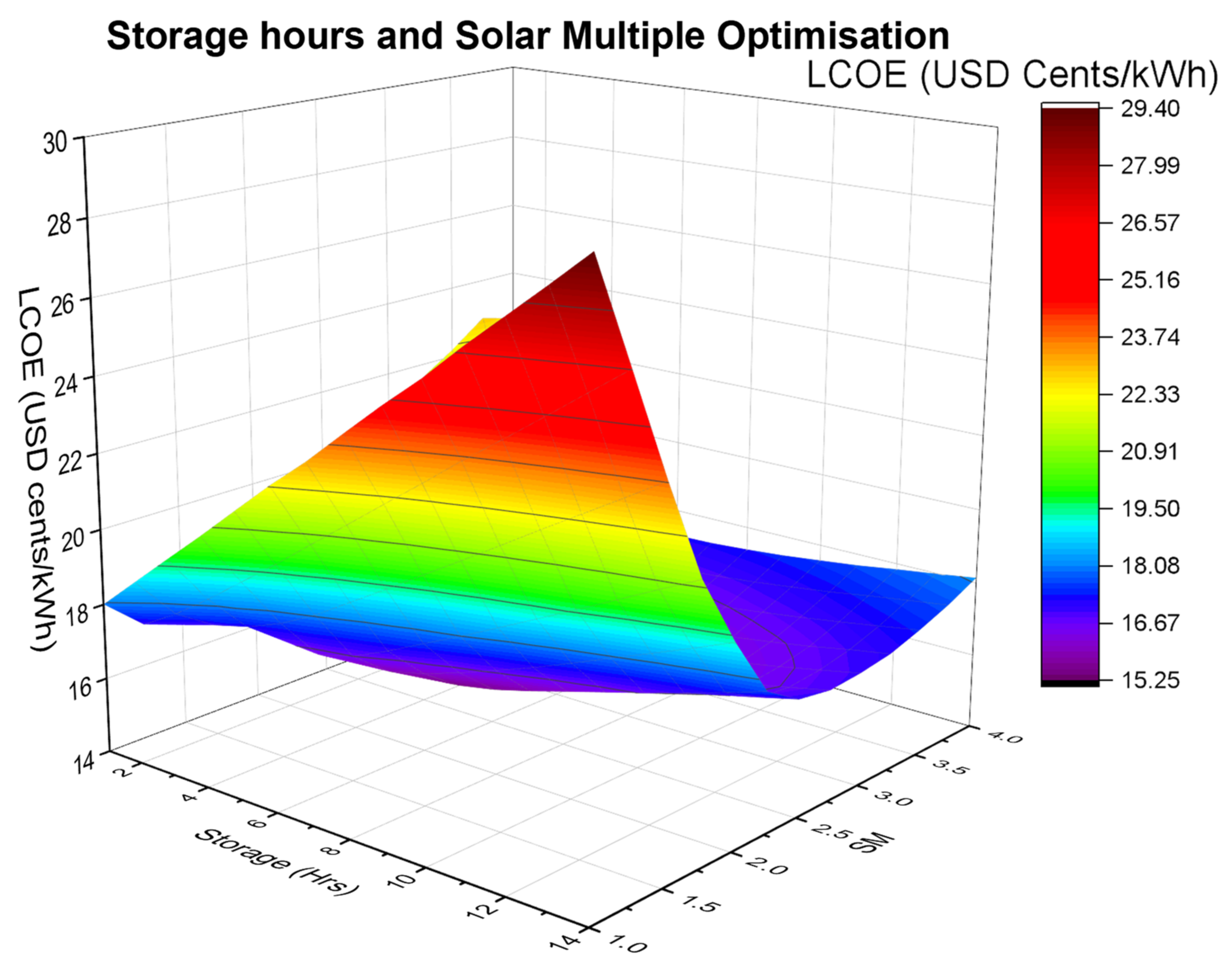
A parametric analysis was carried out to determine the optimum storage hours and solar multiple based on the load profile, location, desired dispatch, and LCOE. The trend from Figure 26 below shows that for low values of SM (1–1.5) the LCOE varies linearly, with a positive gradient, with TES storage hours. For a solar multiple of 2–4, low values of TES storage hours have high LCOE values which start to decrease with an increase in storage hours. The optimum values of LCOE occur for storage hours between 5 and 6 before the trend starts to increase gradually with an increase in storage hours. This is because at low values of storage hours, the energy produced will be too low to justify the investment (the system will be undersized). At high values of storage hours, although the energy produced will be high, the system will be oversized for the application; hence, higher values of LCOE. From the analysis, optimum LCOE occurs at SM = 2.5 and storage hours of 5 h.

Figure 26.
Three-dimensional graph showing the optimisation of the storage hours and the solar multiple.
For the system to cover the period at high-risk from load-shedding, the required storage hours are 5 h (calculated in Section 4.2.1). Therefore, the optimum SM and storage hours chosen for this project are 2.5 and 7 h, respectively—this combination has the lowest LCOE at TES values greater than 5 h.
4.4.2. Technical Performance of the Optimised CSP and TES System
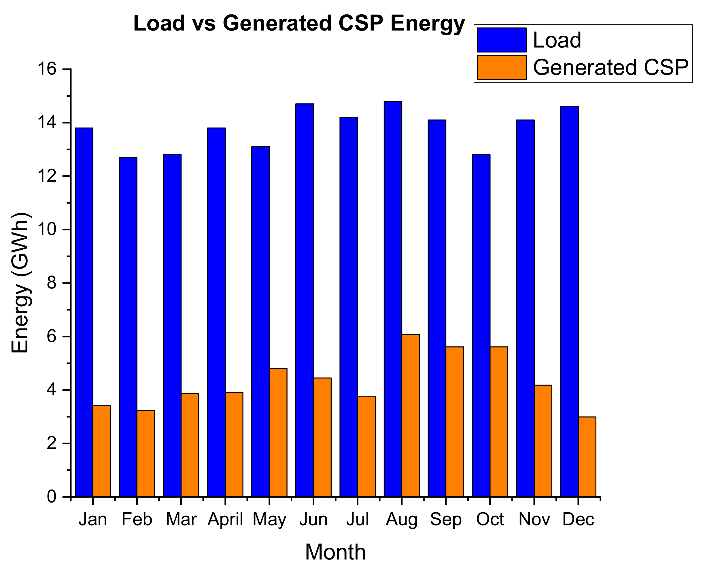
The simulation of the optimised 32 MW gross output, solar multiple of 2.5, storage hours of 7 h at design point of 860 W/m2 predicted a net annual electricity production of 68.4 GWh during the first year of operation. This is approximately 41.3% of the annual demand of the mine at a capacity factor of 40.5%. The predicted capacity factor compares with figures given in IRENA [41] for SM 2.5 and storage of 7 which has values ranging from 42 to 45%. Figure 27 below shows the monthly production of the CSP and TES system vs. the monthly demand of the mine.
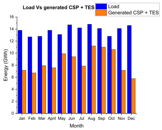
Figure 27.
Monthly generated energy from CSP and TES vs. monthly load.
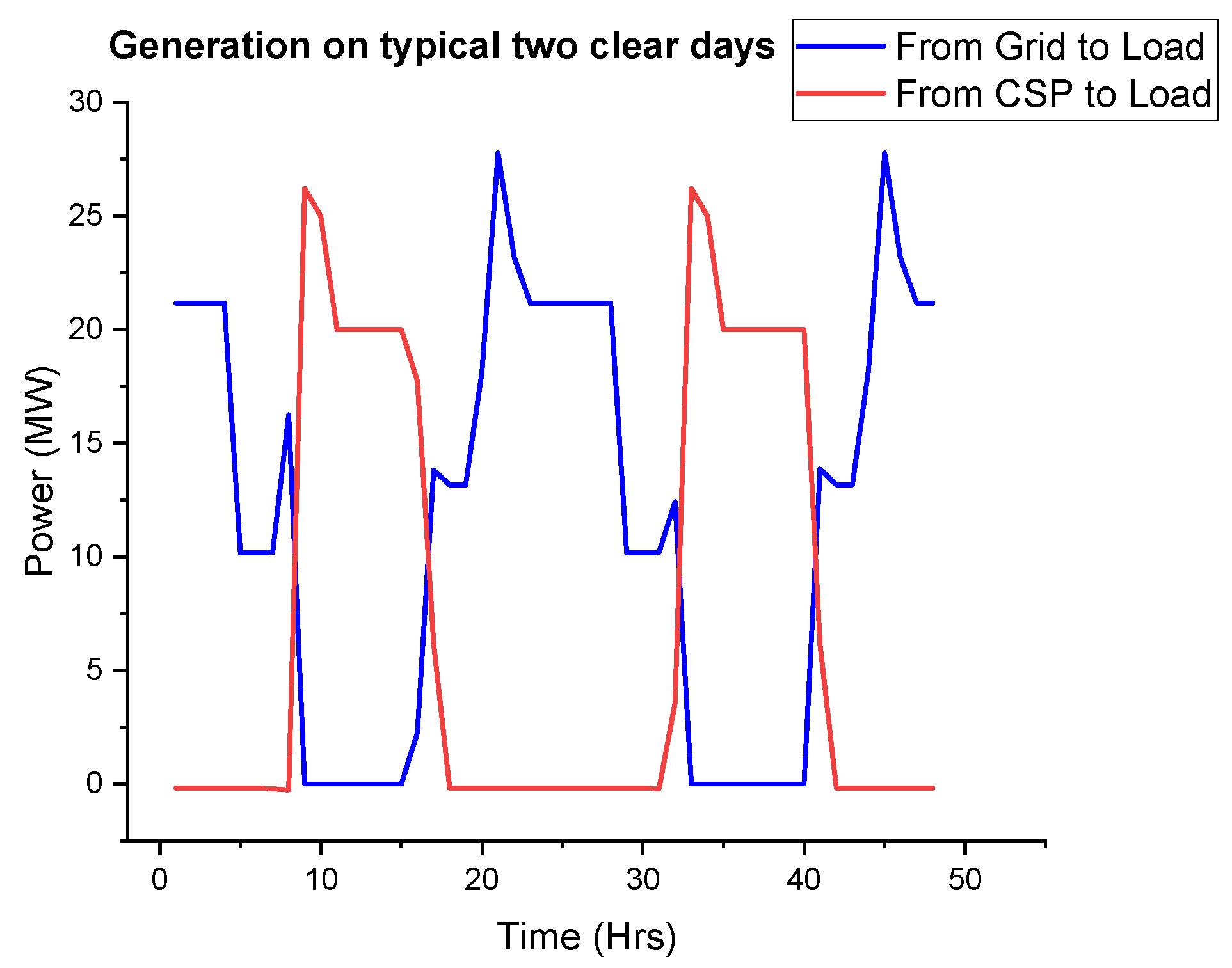
On a typically good day for CSP production, as shown in Figure 28 below, the CSP and TES system is able to supply the load (without the grid) over the designed periods (7 a.m. to 9 p.m.). The grid will supply the load during the off-peak hours.
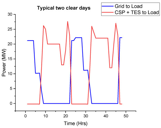
Figure 28.
Two typical consecutive days with good CSP production.
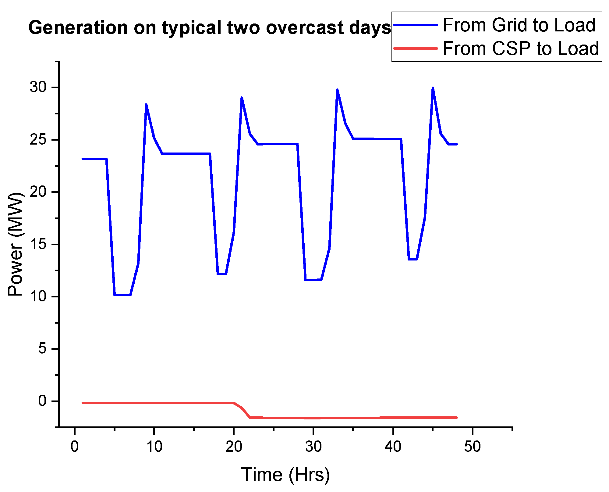
On a typical overcast day, as shown in Figure 29 below, the CSP and TES system will only supply the load from 6 a.m. to 8 a.m. from storage before the grid power covers the slack. The following day, the grid supplies the load without any contribution from the CSP and TES system.
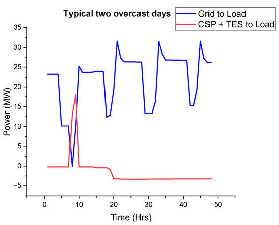
Figure 29.
Two typical consecutive days with bad CSP production.
4.4.3. Economic Performance of Optimised CSP + TES System
The installation cost of the CSP and TES system is predicted at 5593.7/kW. This value is comparable with the IRENA database for CSP systems commissioned in 2019 which showed an installation cost ranging between USD 3704/kW and USD 8645/kW [40]. The predicted LCOE of the system is US cents 15.44/kWh which is lower than the weighted average LCOE (US cents 18.2/kWh) of CSP systems commissioned in 2019. However, the predicted simple pay-back period is 20.9 years with a negative NPV value making the system an unattractive option for investment. Table 18 below shows the main economic indicators of the system.
Table 18.
Economic performance indicators for the CSP and TES system.
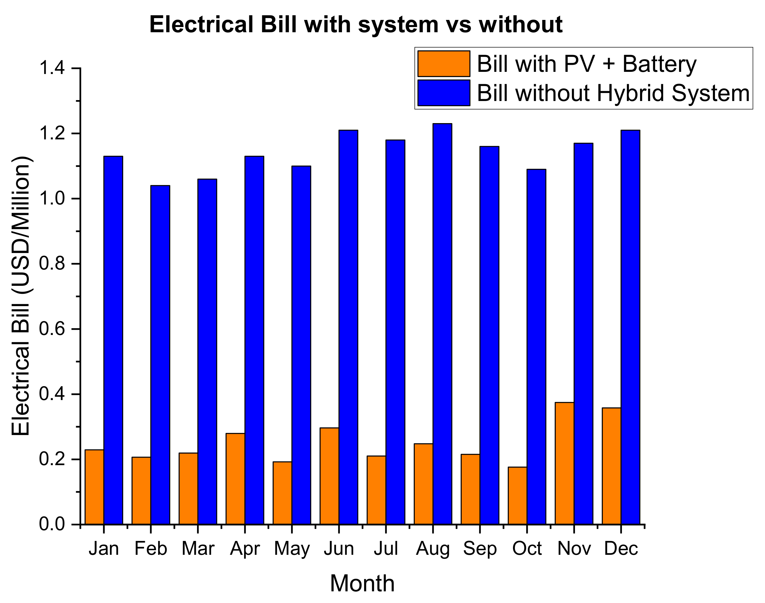
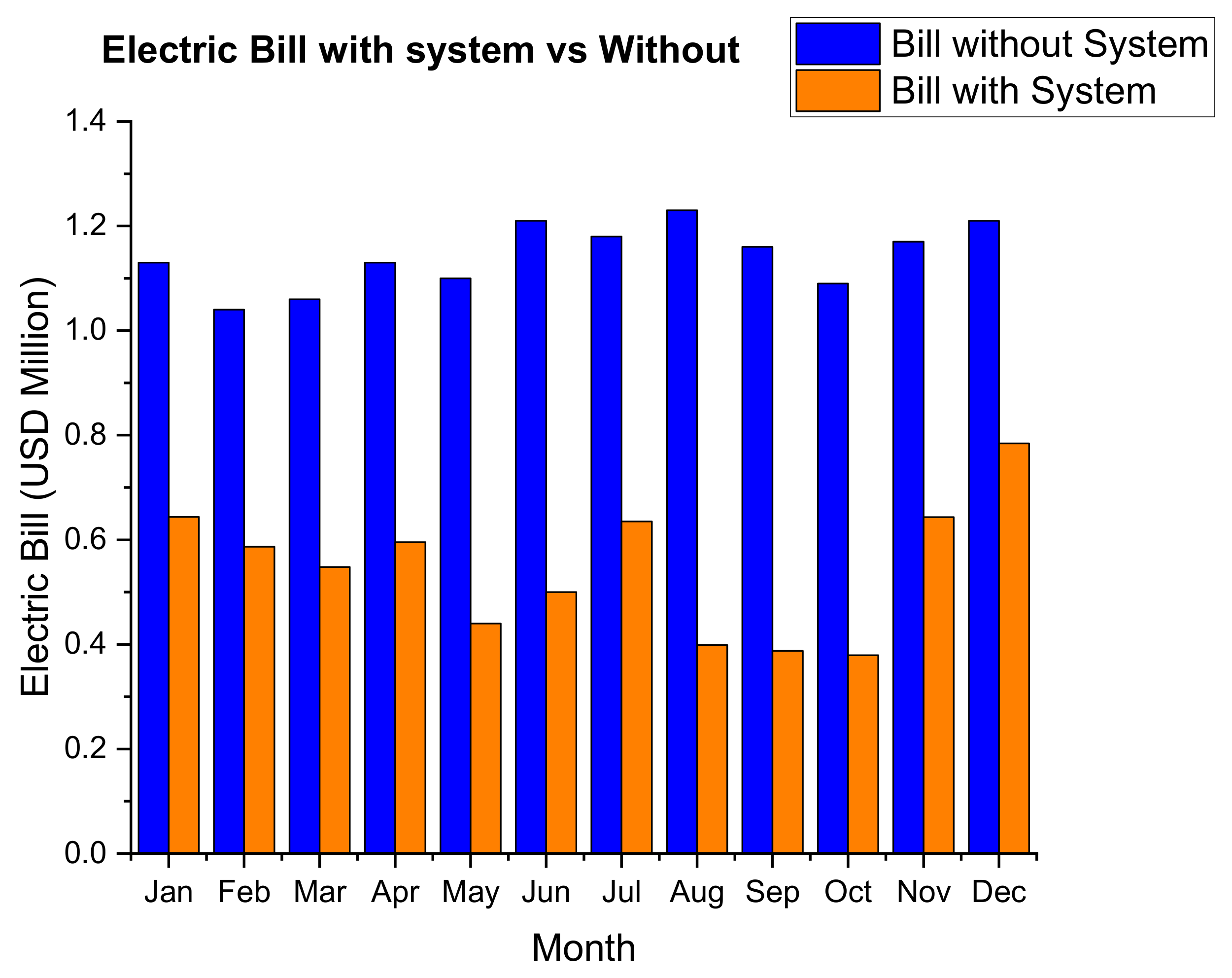
The first-year simulation figures show that the annual electricity bill is reduced from 13.69 million to 6.54 million. This represents a cost reduction of approximately 52.2% on the annual electricity bill after offsetting approximately 41.3% of the annual load. Figure 30 below shows the monthly electricity bill with the CSP and TES system and without.

Figure 30.
Monthly electric bill with the CSP and TES system vs. without.
4.5. System with Exports
The same process (from Section 4.1, Section 4.2, Section 4.3 and Section 4.4) was repeated with the exception that the were no restrictions with exports as described in Section 3.7. The key results are listed in Table 19 below.
Table 19.
Summary of key results.
5. Discussion
5.1. Summary of Results
The Table 19 below shows the summary of key results from the analysis. The key points from the results are:
- The addition of a battery storage system to PV (on a base case scenario) improved the percentage of the load offset by the renewable system and the generated energy by the renewable system by almost double. However, the installation cost, the required land, the LCOE, and the simple pay-back also increased by approximately a factor of 2 while the NPV reduced by nearly half.
- The addition of a thermal storage system to CSP (on a base case scenario) increased the generated energy, capacity factor, and renewable energy contribution by approximately a factor of 2. Moreover, the LCOE improved due to an increase in generated energy. However, the land required for development and the installation costs also nearly doubled.
- For the base case scenario, the CSP and CSP and TES systems have a negative NPV making them commercial unviable options. However, the two systems have positive NPV values for export cases. This concludes that CSP systems become more economically viable as the size of the system (hence generated energy) increases.
- For both cases, the PV system performed better than the CSP system both on the technical performance—generated energy, renewable energy contribution—and economic performance—NPV, LCOE, and simple pay back.
- In general, the systems with exports performed better in terms of technical and economic performance than base case scenarios. This is because the excess energy which could have been clipped is exported gaining revenue in the process.
- For the base case scenario, the PV and battery system performed better than the CSP and TES system in both the technical and economic performances. With the exports scenario, CSP and TES generated more energy (which was largely exported) than the PV and battery system because the simulated battery system was behind the meter. Hence, exports were only limited to the excess energy generated by the PV system. However, due to the high installation costs of the CSP and TES system, the PV and battery system performed better on the economic performance despite producing less energy.
- In terms of renewable energy contribution and grid reliance, the PV and battery system out-performed all the other systems with 63% and 37% (on both scenarios), respectively. The least performing system was the CSP base case.
- In terms of NPV and LCOE, the PV system with exports performed better than the other systems due to a low installation cost and the ability to export energy (hence reduced clipping and grid limit losses). The CSP with no exports performed least on LCOE while CSP and TES with no exports performed least as far as NPV is concerned.
- In terms of land use, the CSP and TES system (with exports) required the biggest land for development while the PV base case required the least.
- As far as the installation cost is concerned, the CSP and TES system has the highest cost while PV system has the lowest. The sensitivity analyses showed that a reduction of about 30% in installation costs will improve the economic performance of the CSP and TES system.
Table 20 below shows the modelled results for LCOE (base case scenario) in comparison to the IRENA power generation costs in 2019 [40] and the Lazard’s levelized cost of energy analysis 2020 [42]. With the exception for the PV and battery results, the modelled results are slightly below or within range of the two references.
Table 20.
Comparison of the LCOE (base case values) with the literature.
From the analysis above, the PV and battery system will be the recommended system for development. This is mainly because the system was able to reduce the annual grid reliance of the mine to only 37% (considering that the dispatch design was not meant to include the off-peak period which constitutes 32% of the annual mine load). The CSP and TES system has the potential to be economically competitive if exports are allowed (hence a bigger capacity) and if the installation costs are reduced by at least 30%.
5.2. Discussion of Results
The object of this report was to analyse the potential of integrating PV (and battery) and CSP (and thermal storage) systems to the Zimbabwean mining sector. The results from the PV and CSP models show that the economic performances of these two are within the predicted figures according to the IRENA renewable cost database for 2019 [40]. However, the technologies do not follow the demand profile for the mine due to their intermittent nature and their unavailability during night-time due to the solar irradiance. This implies that the technologies will not cover the peak period—which is the period suspectable to load-shedding—making it unattractive for implementation.
The addition of the battery to the PV system extended the operational time of the PV system covering the peak hours which are susceptible to load-shedding and the ability to work during cloudy day-time conditions. Similar results were recognised with the addition of thermal storage to the CSP system. However, the difference between the two systems is that the PV and battery system is more profitable which will make it difficult to find investors for the CSP and thermal storage system. It is important to note that the results of the CSP and TES system (export case) shows that if there is high utilisation of the hybrid system, the LCOE of the system decreases (NPV increases) as predicted by Wang [43] and becomes competitive with the PV and battery system. This means this can be an attractive option for very large mines which have a higher demand.
Nationally, the energy yield results from the models show that such a project will be beneficial to the country as whole. Taking for instance the 63% reduction in grid reliance for the PV and battery system, this will mean that this extra energy will be rechannelled to other sectors of the economy improving both productivity and social wellbeing for the benefit of the population. Moreover, the addition of storage (either to PV or CSP) showed that the renewable systems were able to reduce the grid reliance during peak hours, hence the utility will be saved from importing power during this period, thereby using the already in-short supply foreign currency for other sectors of the economy. Moreover, a project of such a magnitude will contribute positively towards the achievement of the national target of having at least 16.5% of overall electricity coming from renewable energy by the year 2025.
6. Conclusions
This research was aimed at analysing the technical and economic performance of CSP (and thermal storage) and PV (and battery storage) as applied to a typical mine in Zimbabwe. The analysis showed that the PV and battery models could offset about 63% of the annual mine load. This is approximately double the contribution of PV system alone as the addition of the battery firmed up the generation of the renewable system. However, there is a need to optimise the PV size relative to the battery storage size (and load profile) as the analysis shows that the larger the capacity of the two systems, the lower the economic performance.
The CSP and TES system managed to offset about 41% of the annual mine load against 24% (base case) of CSP alone. Design parameters such as solar multiple, storage hours, design point DNI, and solar field subsection need to be optimised based on the given demand profile. The analysis shows that CSP systems performed better economically with exports allowed which translates to a bigger plant capacity.
Both the technical and economic performances of all the simulated models were better with the option of exporting to the grid. For models with storage systems, the ability to export energy during peak periods where the electricity tariff is highest certainly boosted the economic performance thereof. With exports, CSP + TES LCOE was comparable to that of PV and battery (US cents 10.45/kWh vs. 9.4/kWh respectively) something that was not the case with no exports (US cents 15.44/kWh vs. 10.67/kWh, respectively).
The installation costs of the CSP systems are currently still high when compared to the PV systems. For instance, the CSP and TES installation cost was over double than that predicted for PV and battery. Moreover, the land required to develop the CSP technology is close to twice the land required for PV systems.
The recommended system based on the analysis carried out will be the PV and battery system. The CSP + TES system shows great potential if the exports to the grid are allowed, if there is a bigger load, and the installation cost falls by at least 30%.
The curve for LCOE is a mirror image of the annual energy with its lowest value (US$0.048/kWh) at a tilt angle of 20°. The highest energy generated was found at an azimuth angle of 00 (North facing) and together with the lowest value of LCOE US5.50/kWh. The annual energy increases steadily up to a GCR of 0.45 where it starts to flatten out. At a GCR of 0.45 the interrow distance is about 2.4 m. The performance ratio of the plant is predicted at 77%. The predicted LCOE of this PV system is USD 0.048/kWh which is comparable to the weighted average LCOE of USD 0.045/kWh in other parts of the world. The 2 h storage battery has 3 PV sizes viable while the 12 h battery storage is only viable for 2 PV sizes. The expected capacity factor of the system is 18.6% with a performance ratio of 75% and a battery roundtrip efficiency of 92.7%. The losses resembled that of the modelled PV with the addition of the battery losses. As with the PV system, the most significant loss was the grid connection limit with a value of around 13%. The optimum solar multiple for the system is 1.25.
7. Future Work
The exports scenario for the PV and battery system was limited to behind the meter battery (due to software limitations) and hence did not fully utilise the potential of the battery system. When simulating in-front of the meter battery in SAM there is no option for the system to supply the local load. There is a need to explore the PV and battery system (in front of the meter hence battery system can export to grid) where exports are allowed while suppling the local load. The system promises to improve the economic performance and the overall generated renewable energy.
The combination of PV and CSP (and battery and TES) also need to be explored. The anticipated benefits from the theory include an improved capacity factor and a reduced LCOE. A dispatch strategy will need to be formulated to exploit the unique characteristics of the systems. SAM software can be used as it has a way to simulate combined cases and a platform to develop a dispatch algorithm to control the combined cases.
The possibility of implementing demand side management at the mine such ass load shifting while evaluating different renewable energy sources need to be analysed. For instance, the possibility of utilising PV during the day to cover most of the load while reducing the peak load, but at the same time exporting the energy from the battery system (during peak period) promises to have great economic benefits.
Author Contributions
Conceptualization, A.M. and P.G.T.; writing—original draft preparation (based on MSc dissertation), A.M.; writing—review and editing, P.G.T., K.J.N. and A.S. All authors have read and agreed to the published version of the manuscript.
Funding
A.M. received a scholarship to study for an MSc at University of Strathclyde from The Beit Trust (Registration 232478).
Institutional Review Board Statement
Not applicable.
Informed Consent Statement
Not applicable.
Data Availability Statement
The data presented in this study is available on request from the corresponding authors.
Acknowledgments
Special thanks go to Mimosa Mining Company for supplying the energy consumption data and load profile. The same appreciation goes to Zimbabwe Electricity Distribution Company for providing the tariff structure.
Conflicts of Interest
The authors declare no conflict of interest but also acknowledge a scholarship from the Beit Trust that was given to the main author to study an MSc program.
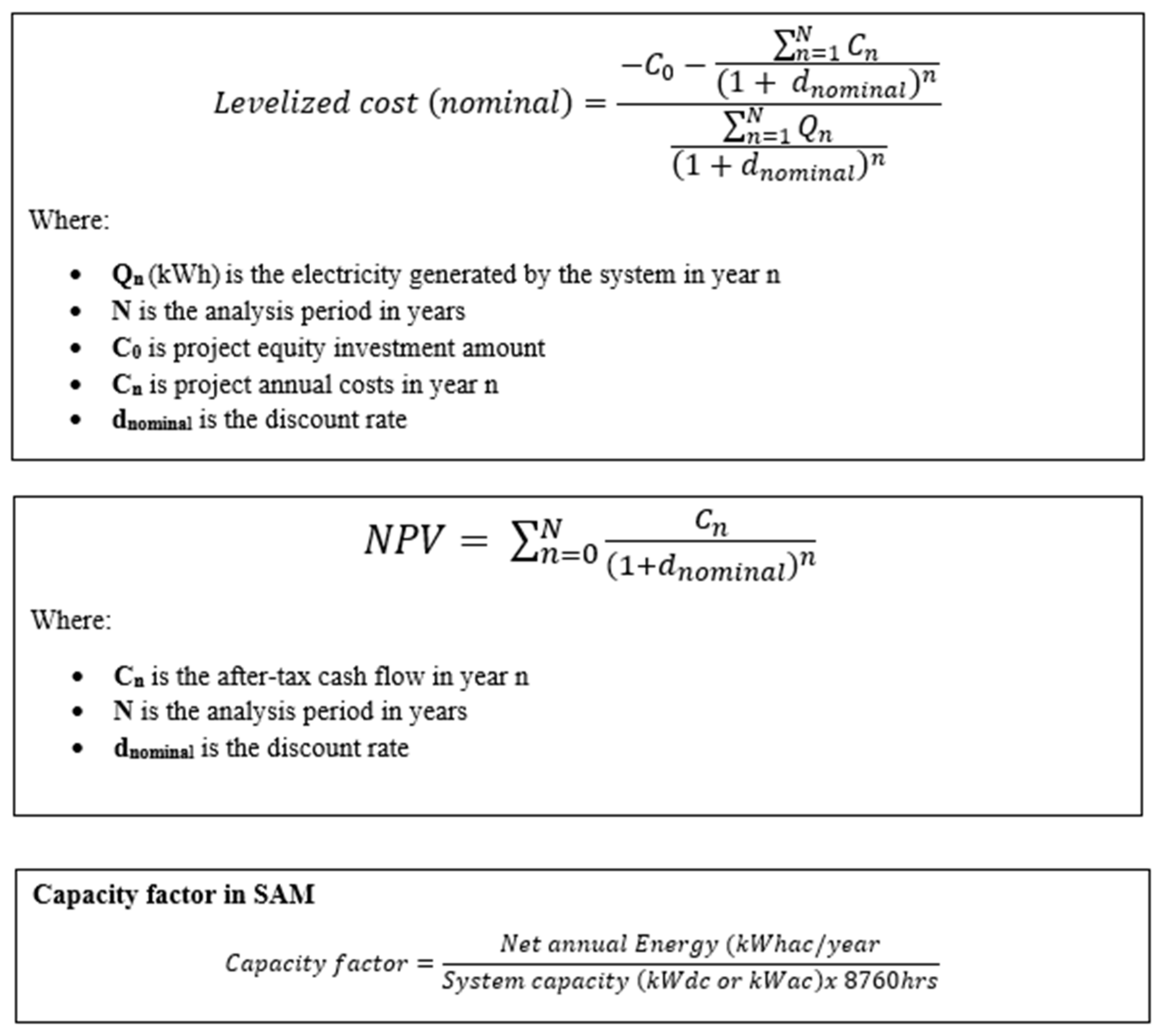
Appendix A. SAM Calculations for LCOE and NPV

Figure A1.
SAM Calculations for LCOE and NPV.
Figure A1.
SAM Calculations for LCOE and NPV.
References
- IEA. Energy Efficiency Indicators Database, Kew World Energy Statistics. Available online: https://www.iea.org/reports/key-world-energy-statistics-2019 (accessed on 21 May 2020).
- Columbia Center on Sustainable Investment. The Renewable Power of the Mine—Accelerating Renewable Energy Integration. Available online: http://ccsi.columbia.edu/files/2018/12/3418-CCSI-RE-and-mining-report-09-lr-reduced-optmized-07-no-links.pdf (accessed on 21 May 2020).
- Australian Renewable Energy Agency. Renewable Energy in the Australian Mining Sector. Available online: https://arena.gov.au/knowledge-bank/renewable-energy-australian-mining-sector/ (accessed on 21 May 2020).
- Zimbabwe Power Company. Available online: http://www.zpc.co.zw/ (accessed on 3 June 2020).
- Ziuka, S.; Seyetin, L.; Mapurisa, B.; Chikodzi, D.; van Kuijk, K. Potential of concentrated solar power (CSP) in Zimbabwe. Energy Sustain. Dev. 2014, 23, 220–227. [Google Scholar] [CrossRef]
- Zurita, A.; Mata-Torres, C.; Valenzuela, C.; Felbol, C.; Cardemil, J.M.; Guzman, A.M.; Escobar, R.A. Techno-economic evaluation of a hybrid CSP + PV plant integrated with thermal storage and a large scale battery energy storage system for base generation. Sol. Energy 2018, 173, 1262–1277. [Google Scholar] [CrossRef]
- Parrado, C.; Girrard, A.; Simon, F.; Fuentealba, E. 2050 LCOE projection for a hybrid PV-CSP plant in the Atacama Desert in Chile. Energy 2016, 94, 422–430. [Google Scholar] [CrossRef]
- Green, A.; Diep, C.; Dunn, R.; Dent, J. High Capacity Factor CSP-PV Hybrid Systems. Energy Procedia 2015, 69, 2049–2059. [Google Scholar] [CrossRef] [Green Version]
- AL-Ghussain, L.; Samu, R.; Taylan, O.; Fahrioglu, M. Techno-Economic Comparative Analysis of Renewable Energy Systems: Case study in Zimbabwe. Inventions 2020, 5, 27. [Google Scholar] [CrossRef]
- Schoniger, F.; Thonig, R.; Resch, G.; Lilliestam, J. Making the sun shine at night: Comparing the cost of dispatchable Concentrating solar power and photovoltaics with storage. Energy Sources 2021, 16, 55–74. [Google Scholar] [CrossRef]
- Lovegrove, K.; James, G.; Leitch, D.; Milczareck, A.; Rutovitz, J.; Watt, M.; Wyder, J. Comparison of Dispatachable Renewable Electricity Options; Australian Renewable Energy Agency: Canberra, Australia, 2018. Available online: https://arena.gov.au/assets/2018/10/Comparison-Of-Dispatchable-Renewable-Electricity-Options-ITP-et-al-for-ARENA-2018.pdf (accessed on 17 May 2021).
- Jorgenson, J.; Mehos, M.; Denholm, P. Comparing the net cost of CSP-TES to PV deployed with battery storage. AIP Conf. Proc. 2016, 1734, 080003. [Google Scholar]
- Alves, W.; Ferreira, P.; Araujo, M.; Souza, J. Renewable energy for sustainable mining. Int. J. Qual. Res. 2020, 14, 593–600. [Google Scholar] [CrossRef]
- Igogo, T.; Lowder, T.; Engel-Cox, J. Integrating Clean Energy in Mining Operations: Opportunities, Challenges, and Enabling Approaches; Joint Institute for Strategic Energy Analysis: Golden, CO, USA, 2020; NREL/TP-6A50-76156. [Google Scholar]
- Nasirov, S.; Agostin, A.C. Mining experts’ perspectives on the determinates of solar technologies adoption in the Chilean mining industry. Renew. Sustain. Energy Rev. 2018, 95, 194–202. [Google Scholar] [CrossRef]
- Zharan, K.; Bongaerts, J.C. Decision making on the integration of renewable energy in the mining industry: A case study analysis, a cost analysis and a SWOT analysis. J. Sustain. Min. 2017, 16, 162–170. [Google Scholar] [CrossRef]
- Ellabban, O.; Alassi, A. Optimal hybrid microgrids sizing framework for the mining industry with three case studies from Australia. IET Renew. Power Gener. 2021, 15, 409–423. [Google Scholar] [CrossRef]
- Pollack, K. Renewable Energy for the Mining Industry: Trends and Developments, ResearchGate 2017. Available online: https://www.researchgate.net/publication/327931783_Renewable_Energy_for_the_Mining_Industry_Trends_and_Developments (accessed on 5 June 2021).
- Liu, J.; Jin, T.; Liu, L.; Chen, Y.; Yuan, K. Multi-Objective Optimisation of a hybrid ESS based on Optimal Energy Management strategy for LHDs. Sustainability 2017, 9, 1874. [Google Scholar]
- Kalantari, H.; Ghoreishi-Madiseh, S.A.; Sasmito, A.P. Hybrid Renewable Hydrogen Energy Solution for application in Remote Mines. Energies 2020, 13, 6365. [Google Scholar] [CrossRef]
- Boyse, F.; Causevic, A.; Duwe, E.; Orthofer, M. Sunshine for Mines: Implementing Renewable Energy for Off-grid Operations. Available online: https://rmi.org/wp-content/uploads/2017/04/CWR14_MinesReport_singles.pdf (accessed on 6 June 2021).
- Zharan, K.; Bongaerts, J.C. Survey Research on Integrating Renewable Energy into the Mining Industry. In Proceedings of the ISES Conference Proceeding, Abu Dhabi, United Arab Emirates, 29 October–2 November 2017; Available online: http://proceedings.ises.org/paper/swc2017/swc2017-0142-Zharan.pdf (accessed on 5 June 2021).
- Energy and Mines, Congress Report and Presentations 2020. Available online: https://issuu.com/energyandmines/docs/energy_and_mines_report_design_final_draft (accessed on 5 June 2021).
- Mining Review Africa. Issue 2. 2021. Available online: https://www.miningreview.com/issues/mining-review-africa-issue-2-2021/ (accessed on 6 June 2021).
- Gangazhe, T. Barriers to Greater Adoption of Renewable Energy by Mining Companies in South Africa. Master’s Thesis, Gordon Institute of Business Science, University of Pretoria, Pretoria, South Africa, 2016. [Google Scholar]
- Tazay, A. Techno-Economic Feasibility Analysis of a Hybrid Renewable Energy Supply Options for University Buildings in Saudi Arabia. Open Eng. 2021, 11, 39–55. [Google Scholar] [CrossRef]
- Jeyasudha, S.; Krishnamoorthy, M.; Saisandeep, M.; Balasubramanian, K.; Srinivasan, S.; Thaniaknti, B.S. Techno economic performance analysis of hybrid renewable electrification system for remote villages of India. Int. Trans. Electr. Energy Syst. 2020. [Google Scholar] [CrossRef]
- Weiwu, M.; Xinpei, X.; Gang, L. Techno-economic evaluation for hybrid renewable energy system: Application and merits. Energy 2018, 159, 385–409. [Google Scholar]
- Ammari, C.; Belatrache, D.; Touhami, B.; Makhloufi, M. Sizing, optimization, control and energy management of hybrid renewable energy system—A review. Energy Built Environ. 2021. [Google Scholar] [CrossRef]
- SAM Help Manual. Available online: https://sam.nrel.gov/download.html (accessed on 14 June 2020).
- Beuse, M.; Dirksmeier, M.; Steffen, B.; Schmidt, T.S. Profitability of commercial and industrial photovoltaics and battery projects in South-East Asia. Appl. Energy 2020, 271, 115218. [Google Scholar] [CrossRef]
- Solcast. Available online: https://solcast.com/ (accessed on 14 June 2020).
- Homer Help Manual. Available online: https://www.homerenergy.com/products/pro/docs/index.html (accessed on 10 June 2020).
- National Renewable Energy laboratory (NREL). Technical Report NREL/TP-6A20-60272. Available online: https://www.nrel.gov/docs/fy14osti/60272.pdf (accessed on 6 June 2020).
- PVSyst Help Manual. Available online: https://www.pvsyst.com/help/ (accessed on 14 June 2020).
- Zurita, A.; Mata-Torres, C.; Cardemil, J.M.; Escobar, A.R. Assessment of time resolution impact on the modelling of a hybrid CSP-PV plant: A case of study in Chile. Sol. Energy 2020, 202, 553–570. [Google Scholar] [CrossRef]
- Bayod-Rujula, A.A.; Haro-Larrode, M.E.; Martinez-Gracia, A. Sizing criterio of hybrid photovoltaic-wind systems with battery storage and self-consumption considering interaction with the grid. Sol. Energy 2013, 98, 582–591. [Google Scholar] [CrossRef]
- Petrollese, M.; Cocco, D. Optimal design of a hybrid CSP-PV plant for achieving the full dispatchability of Solar Energy power plants. Sol. Energy 2016, 137, 447–489. [Google Scholar] [CrossRef]
- Turchi, C.S.; Boyd, M.; Kesseli, D.; Kurup, P.; Mehos, M.; Neises, T.; Sharan, P.; Wagner, M.; Wendelin, T. CSP Systems Analysis––Final Project Report; NREL/TP-5500-72856; National Renewable Energy Laboratory: Golden, CO, USA, 2019. Available online: https://www.nrel.gov/docs/fy19osti/72856.pdf (accessed on 16 June 2020).
- International Renewable Energy Agency (IRENA). Renewable Power Generation Costs in 2019. Available online: https://www.irena.org/publications (accessed on 16 June 2020).
- International Renewable Energy Agency (IRENA). Renewable Energy Technologies (CSP): Cost Analysis Series, Volume 1: Power Sector, Issue 215. Available online: https://www.irena.org/documentdownloads/publications/re_technologies_cost_analysis-csp.pdf (accessed on 16 June 2020).
- Lazard’s Levelized Cost of Energy Analysis, Version 14.0. Available online: https://www.lazard.com/perspective/levelized-cost-of-energy-and-levelized-cost-of-storage-2020/ (accessed on 17 May 2021).
- Wang, Z. Chapter 6—Thermal Storage Systems, Design of Solar Thermal Power Plants; Academic Press: Cambridge, MA, USA, 2019; pp. 387–415. [Google Scholar]


Publisher’s Note: MDPI stays neutral with regard to jurisdictional claims in published maps and institutional affiliations. |
© 2021 by the authors. Licensee MDPI, Basel, Switzerland. This article is an open access article distributed under the terms and conditions of the Creative Commons Attribution (CC BY) license (https://creativecommons.org/licenses/by/4.0/).